Research and application of high-resolution micro-cylindrically focused logging tool

The unknown nature and complexity of non-uniform formations cause new difficulties and challenges to the accurate detection of electrical instruments in shallow formations. The micro-cylindrically focused logging tool (MCFL) can provide three original measurement curves, RB0, RB1, and RB2, with different detection depths, which reflect the flushing zone resistivity, mudcake resistivity, and mudcake thickness. In this study, the finite element method was used to model and analyze the micro-cylindrically focused logging tool tool in a three-dimensional non-uniform medium model. By converting the partial differential equation into a generalized polar problem, the logging response characteristics of the micro-cylindrically focused logging tool tool at different detection depths and ranges, mudcake thicknesses, flush zones, and mudcake resistivity contrasts were investigated. Inverse processing of the micro-cylindrically focused logging tool data using the least-squares method was used to obtain the flush zone resistivity, mudcake resistivity, and mudcake thickness, based on which the micropotential and microgradient curves were synthesized. In addition, a digital focusing method was proposed to improve the focusing accuracy and flexibility of the instrument, enhancing the performance of the micro-cylindrically focused logging tool. The optimized design of the focusing method significantly improved the detection performance of the pole plate. This plays an important role in the evaluation of thin layers and oil-water reservoirs.

1 Introduction

Wash zone resistivity is an essential parameter in petroleum resource exploration and is important for formation evaluation (Tian et al., 2003; Salazar and Torres-Verdin, 2009) Although certain array logging methods, such as array induction (Wang, 2003; Li et al., 2012; Zhou et al., 2016; Bai et al., 2018) and lateral logging (Li et al., 2010; Zhao et al., 2019; Zhu et al., 2019), can detect formation features at different radial depths, their greater detection depths pose difficulties in the accurate evaluation of mudcake and electrical parameters in shallow formations. To finely measure the resistivity of shallow formations, resistivity logging instruments achieve a reduced detection depth by reducing the electrode distance. Traditional micro-resistivity logging methods, such as micro-resistivity logging (Gao et al., 2017; Xing et al., 2018), micro-laterolog (Chen and Nie, 1997), and micro-spherically focused logging (Wang and Wu, 1994; Zeng et al., 2010; Ren et al., 2021), can be used to measure the resistivity and mudcake parameters in the flushing zone. However, the application of existing micro-resistivity logging methods is limited because they can only detect the electrical parameters of shallow formations at a single radial depth. They could not obtain the variation pattern of the formation properties in the radial direction. In addition, during actual logging, pole plates are easily damaged in horizontal or high-temperature wells because of the use of soft pole plates (Zhou, 2003; Xia et al., 2015). Therefore, a more advanced micro-resistivity logging method is urgently needed in actual logging operations that can efficiently measure the shallow resistivity of the formation and simultaneously realize the data acquisition of resistivity at multiple radial depths.

The micro-cylindrically focused logging (MCFL) tool is a focused shallow-probe resistivity logging instrument that can compensate for the shortcomings of existing logging methods (Hao and Sun, 2017). Unlike other resistivity logging methods, the MCFL emission current is independently focused in planes parallel and perpendicular to the tool axis, reducing sensitivity to borehole geometry, and its pole plate shape and leading-edge isotope are semi-cylindrical to better fit the borehole shape. In addition, the instrument can achieve both a multi-path detection depth and high axial resolution at shallow formation depths and can reasonably estimate mudcake and mud parameters by accurately measuring the radial variation of shallow resistivity. Therefore, MCFL has high research significance and application value. The MCFL tool was first proposed 30 years ago by Schlumberger Technology. Domestic and foreign experts and scholars have conducted research on orthorectified modeling, mudcake parameter calibration, and inversion methods of the instrument in the following decades (Donadille et al., 2017; Li et al., 2017; Hao et al., 2018). However, to date, only a few documents have been published on core technologies. Domestic research on MCFL tool hasn’t yet been popularized in practical applications, and there is still a large gap compared with advanced foreign focused resistivity measurement instruments. Therefore, it is a very worthwhile task to break the current lack of relevant reliable technology in China and independently develop internationally competitive micro-cylindrically focused logging tool. In addition, since the beginning of development, MCFL instrument adopts hard focusing method in focusing, which leads to the residual potential not equal to 0 in the actual focusing process, i.e., the residual voltage cannot be eliminated, and the focusing effect is poor, which in turn affects the logging effect of the instrument (Guo et al., 2021).

To improve the measurement accuracy and longitudinal resolution of the instrument, the polar plate focusing method of the MCFL tool must be modified. In this study, a digital focusing method was proposed to realize microresistivity measurements and improve the longitudinal resolution of the instrument by enhancing the focusing accuracy. Furthermore, the resistivity response of the MCFL is non-linearly related to the formation parameters, and the measurement data of the MCFL cannot be processed using simple coefficient correction and crossplots. In this study, the definite solution of the partial differential equation was transformed into a functional extremum problem. Considering the influence of mudcake resistivity, mudcake thickness, and flushing resistivity, the response of the micro-cylindrically focused logging tool was forward simulated using the three-dimensional (3D) finite element method. Finally, the measured data were inverted based on the least-squares method, and the mudcake parameters were corrected based on the inversion results.

2 Working principle of MCFL

MCFL is a semi-cylindrical focus with a semi-cylindrical isotropic surface at the center front of the pole plate (Hao et al., 2018). This focus is suitable for the geometry of the borehole and mudcake and can provide improved resistivity measurements of the flush zone. The MCFL can provide three raw measurement curves, R_B0, R_B1, and R_B2, at different probing depths, reflecting the mudcake thickness, resistivity, and flush zone resistivity. The apparent resistivity obtained from the MCFL was highly accurate and could be used to accurately estimate the resistivity and thickness of the mudcake, making it more suitable for the interpretation and evaluation of permeable formations. The pole-plate structure and working principle of the instrument are shown in Figure 1.

FIGURE 1

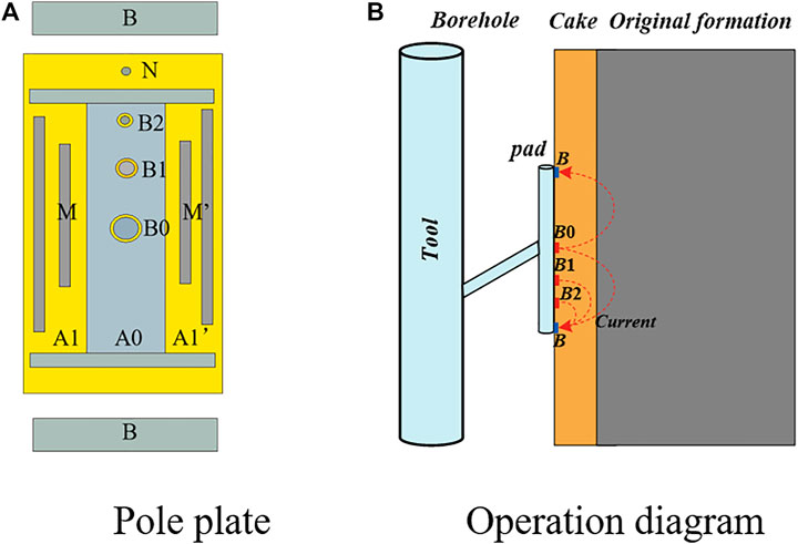
FIGURE 1. Schematic diagram of microcolumn focusing logging tool. (A) MCFL electrode structure diagram, A0 is the main electrode. B0, B1, B2 are the emission electrode. M and M′ is the monitoring electrode, N is the potential reference electrode, and B is the loop electrode. (B) The working principle of MCFL is that the micro-column plate is close to the mud cake, and the current values of button electrodes B0, B1, and B2 can measure the apparent resistivity of the formation at different radial depths.

A0 is the main electrode. B0, B1, and B2 are the emitter electrodes separated from A0 by an insulating layer. M and M′ are the supervisory electrodes, N is the potential reference electrode, B is the loop electrode, and Pad is the micropolar plate.

The working principle of MCFL is shown in Figure 1b. Main electrode A0, which occupies a larger area in the middle of the pole plate, provides the main shielding current to the formation, and the current returns to electrode B. Pole plate A0 has significant length in the longitudinal direction, ensuring the longitudinal passive focus of measurement button electrodes B0, B1, and B2. Long electrodes A1 and A1′ on the outside of the pole plate are driven by the current amplification channel to provide a shielding current injection into the ground layer. The size of the shielding current is controlled to ensure that the potential of supervisory electrode M between main electrode A0 and shielding electrode A1 (A1′) is equal to the potential of main electrode A0, thus achieving the measurement of button electrodes B0, B1, and B2 for lateral active focusing. The shielding current amplification channel is applied to amplify potential difference U_MA0 between A0 and M (M′) appropriately to adjust shielding current I_S until the potentials of A0 and M were the same, thus, the main shielding current from A0 is focused in the radial direction, and the propagation path is through the mudcake, reaching the intrusion zone formation before dissipating back to B. The apparent resistivity of the measuring electrode can then be used as the flushing zone resistivity. Pole plate A0 is separated from the three button electrodes, B0, B1, and B2, by an insulating layer. To meet the equipotential of main electrodes A0 and B0, B1, and B2, the following circuit design was used, and a small resistor was used to short-circuit them during the power supply and measurement. The middle of electrode A0 and loop electrode B is measurement reference electrode N, which is equipotential to the ground-flushing zone. Current value I_B0 of electrode B0 and potential difference U_MN between supervisory electrode M and reference electrode N, which is equipotential to main electrode A0, were collected, and the apparent resistivity value of the intrusion zone was obtained using Eq. 1:

$R_{B0}=k_0\frac{U_{MN}}{I_{B0}}(1)$

Where, $k_0$ is the scale factor of button electrode $B0$, $R_{B0}$ is the apparent resistivity of the intrusion zone, $I_{B1}$ is the current value, and $U_{MN}$ is the potential difference between the monitoring electrode M and the reference electrode N. Similarly, current values $I_{B1}$ and $I_{B2}$ were measured for button electrodes $B1$ and $B2$, respectively, to determine the apparent resistivity of the strata at different radial depths.

3 MCFL response simulation analysis

Owing to the complex structure of the MCFL pole plate instrument and the existence of multiple electrode sizes, multi-scale electromagnetic modeling in complex non-homogeneous media is required. The finite element method has the advantages of flexible fitting of complex boundary conditions and variable stability of the numerical solution, which is suitable for addressing logging response problems in non-homogeneous media with complex boundaries and excitation forms.

The calculation simulation model is a 3D non-uniform formation model because the instrument adopts the push-to-rest approach to the formation, as shown in Figure 2. In the figure, Rxo is the flushing zone resistivity, Rmc is the mudcake resistivity, and Hmc is the mudcake thickness.

FIGURE 2

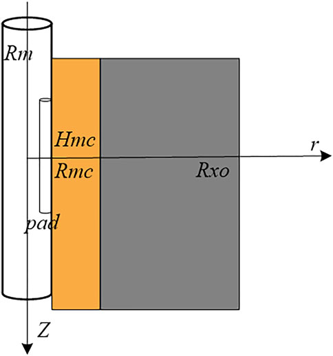
FIGURE 2. Three-dimensional heterogeneous medium formation model. In the figure, Rxo is the flushing resistivity. Rmc is the mud cake resistivity. Hmc is the mud cake thickness, and Pad is the MCFL plate.

3.1 Numerical simulation

The MCFL pushes against a polar plate when the formation is not axisymmetric and can only be analyzed using 3D numerical simulation methods (Merchant et al., 2006).

Potential function $U\left(x,y,z\right)$ at any point in each region where resistivity $\rho$ is equal to a constant should satisfy the differential equation (Deng et al., 2010; Wu et al., 2022):

$\frac{\partial }{\partial x}\left(\frac{1}{\rho }\frac{\partial U}{\partial x}\right)+\frac{\partial }{\partial y}\left(\frac{1}{\rho }\frac{\partial U}{\partial y}\right)+\frac{\partial }{\partial z}\left(\frac{1}{\rho }\frac{\partial U}{\partial z}\right)=0(2)$

At the surface of the constant pressure electrode and at the infinitely far boundary, U satisfies the first type of boundary condition and obeys the complete constraint condition. At the surface of the constant current electrode, it satisfies the second type of boundary condition.

On the surface of electrode A0:

$\underset{A0}{\iint }\frac{1}{\rho }\frac{\partial U_{A0}}{\partial n}ds=I_0,U_{A0}=const(3)$

Where, $U_{A0}$ represents the electric potential of electrode $\mathrm{A}0$, whose value is constant. $I_0$ represents the current of electrode A0. N represents normal vector, s is the metal surface.

On the surface of supervised electrode M and M':

$\underset{M\left(M^{\prime }\right)}{\iint }\frac{1}{\rho }\frac{\partial U_{M\left(M^{\prime }\right)}}{\partial n}ds=0,U_{M\left(M^{\prime }\right)}=U_{A0}(4)$

Shielding electrode A1 and A1´ surface:

$\underset{A1+A{1}^{\prime }}{\iint }\frac{1}{\rho }\frac{\partial U_{A1\left(A{1}^{\prime }\right)}}{\partial n}ds=I_1,U_{A1\left(A{1}^{\prime }\right)}=const(5)$

Where, I₁ represents the current of electrode A1 and A1´.

On the surface of the three button electrodes B0, B1, and B2:

$\underset{B0\left(B1,\mathrm{B}2\right)}{\iint }\frac{1}{\rho }\frac{\partial U_{B0\left(B1,B2\right)}}{\partial n}ds=I_{B0\left(B1,\mathrm{B}2\right)},U_{B0}=U_{B1}=U_{B1}=U_{A0}(6)$

On the surface of reference electrode N:

$\underset{N}{\iint }\frac{1}{\rho }\frac{\partial U_N}{\partial n}ds=0,U_N=const(7)$

On the surface of circuit electrode B:

$\underset{B}{\iint }\frac{1}{\rho }\frac{\partial U_B}{\partial n}ds=-\left(I_0+I_1+I_{B0}+I_{B1}+I_{B2}\right),U_B=const(8)$

The equivalent variational problem of the general boundary value problem is given by the following formula (Jin, 1998):

$\delta F\left(U\right)=0(9)$

$\begin{array}{c}F\left(U\right)=\frac{1}{2}{\iiint }_{\mathrm{\Omega }}\left[\frac{1}{\rho }{\left(\frac{\partial U}{\partial x}\right)}^2+\frac{1}{\rho }{\left(\frac{\partial U}{\partial y}\right)}^2+\frac{1}{\rho }{\left(\frac{\partial U}{\partial z}\right)}^2+\beta U^2\right]d\mathrm{\Omega }\\ +{\iint }_S\left(\frac{\gamma }{2}{U}^2-qU\right)dS-{\iiint }_{\mathrm{\Omega }}fUdU\end{array}(10)$

Where, F (•) represents the functional of the potential function U(x, y, z). β represents the known parameters related to the physical properties of the region. γ and q represent the known parameters related to the physical properties of the boundary. F represents the source or excitation function. When U satisfies the first boundary condition, the second term at the right end of the functional F(U) can be expressed as:

${\iint }_S\left(\frac{\gamma }{2}{U}^2-qU\right)dS=-{\displaystyle \sum }_A{I}_A{U}_A(11)$

At the same time, when f=0, β=0, the fixed solution problem can be converted to the functional extreme value problem. We find:

$F\left(U\right)=\frac{1}{2}\underset{\mathrm{\Omega }}{\iiint }\frac{1}{\rho }\left[{\left(\frac{\partial U}{\partial x}\right)}^2+{\left(\frac{\partial U}{\partial y}\right)}^2+{\left(\frac{\partial U}{\partial z}\right)}^2\right]d\mathrm{\Omega }-{\displaystyle \sum }_A{I}_A{U}_A(12)$

Where, Ω represents the integral region of triple integral.

The finite-element solution includes area and function discretization. In finite element partitioning, denser nodes are set on the electrode system, and thinner nodes are set outside the electrode system. The value of the potential function on each node of the partitioned unit is approximated using an appropriate interpolation method, which transforms the generalized function into a quadratic one containing the potential function on each node. When the generalized function takes an extremely small value, the potential distribution at each node is an approximate solution of the actual electromagnetic field. When calculating the MCFL response, the method of “eliminating elements” while “installing” is used, where all the elements of this line are calculated and written to the hard disk. After all the elements are installed and written to the hard disk, the problem is solved using back substitution.

The forward parameters are shown in Table 1. The adaptive mesh generation method is adopted. Dense grid is used near the electrode, while uneven sparse grid is used outside the electrode plate to speed up the calculation.

TABLE 1

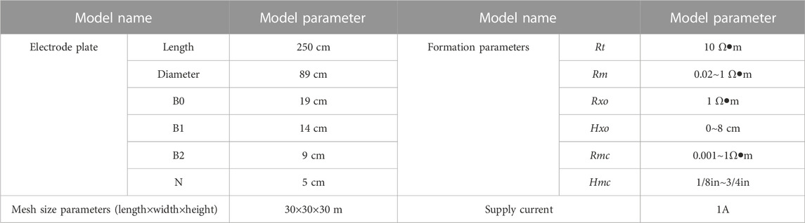
TABLE 1. 3D inhomogeneous formation model parameters.

3.2 Analysis of the detection range of the MCFL tool

The radial detection depth and intrusion impact of the MCFL can be described by the pseudo-geometry factor, and pseudo-geometry factor J of the button electrode is expressed as follows.

$J=\frac{Ra-R_t}{R_{xo}-R_t}(13)$

Where, Ra denotes the apparent resistivity of the button electrode, Rt denotes the in-situ formation resistivity, Rxo denotes the formation washout zone resistivity, and J is the pseudo-geometric factor. The intrusion depth corresponding to pseudo-geometric factor J = 0.50 is used as the detection depth of the MCFL. The intrusion depth corresponding to pseudo-geometry factor J = 0.95 is used as the detection range. The pseudo-geometric factor curve of the MCFL is shown in Figure 3.

FIGURE 3

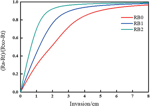
FIGURE 3. Pseudo-geometry factor of MCFL. The MCFL has three different detection depths in the radial direction. B0 has the maximum detection depth and can effectively evaluate the resistivity characteristics of the washed zone formation. B1 and B2 are closer to the loop electrode and have a small detection depth, which can be used for parameter estimation and influence correction of mud and mud cake.

The horizontal axis in Figure 3 indicates the intrusion depth, and the vertical axis indicates the pseudo-geometric factor of the three button resistivities. As seen from the figure, the MCFL has three different probing depths in the radial direction: 1.94 cm for electrode B0, 1.16 cm for electrode B1, and 0.65 cm for electrode B2. The probing ranges of electrodes B0, B1, and B2 were 7.0, 5.0, and 3.0 cm, respectively. Among them, B0 has the greatest detection depth, which can effectively evaluate the electrical characteristics of wash zone formation. Electrodes B1 and B2 have a more limited detection depth because they are closer to the loop electrode and can be used for parameter estimation and influence the correction of mud and mudcake parameters.

3.3 MCFL calibration plate

3.3.1 Mudcake correction plate

To study the effect of MCFL on mudcake, the RB0, RB1, and RB2 logging responses with different mudcake thicknesses, intrusion zones, and resistivity contrasts were calculated using the finite element method. The calculation results are shown in Figure 4, where the horizontal axis indicates the resistivity ratio of the intrusion zone to the mudcake, and the vertical axis indicates the ratio of apparent resistivity to mudcake resistivity.

FIGURE 4

FIGURE 4. Plate of mudcake thickness correction. (A) B0 electrode (B) B1 electrode (C) B2 electrode. The figure shows that the thicker the mud cake, the greater the influence of the mud cake on the apparent resistivity measured by the MCFL. The sensitivity of the resistivity measured by the three electrode plates to the mud cake parameters is different. B2 electrode is the most affected by the mud cake, followed by B1 and B0.

As shown in Figure 4, the thicker the mudcake is, the greater its influence on the apparent resistivity measured by the MCFL. When the mudcake thickness was less than 1/4 in (1 in =2.54 cm), RB0 was less affected, and the apparent resistivity of RB0 was slightly different from the resistivity of the intrusion zone. When the mudcake thickness was greater than 1/4 in, RB0, RB1, and RB2 were all affected, resulting in an increasing deviation between the apparent resistivity and actual ground resistivity. The magnitude of this deviation also reflects the different sensitivities of the three logging responses to the mudcake parameters, with electrode B2 being the most influenced by the mudcake, B1 the second most influenced, and B0 the least influenced. The three resistivity response curves exhibit a non-linear relationship with Rxo/Rmc. The smaller the detection depth is, the stronger the non-linearity.

3.3.2 Mud calibration plate

To investigate the effect of the borehole mud on the apparent resistivity response measured by the micro-cylindrically focused instrument, the formation model was divided into two layers in the radial direction: the borehole mud and uniform formation outside the mud. The resistivity of the uniform formation outside the mud (flushing zone resistivity) was set to 1 Ω•m. The resistivity of the borehole mud Rm was continuously changed to 0.02, 0.05, 0.1, 0.2, 0.5, and 1 Ω•m, and we observed the change of apparent resistivity with borehole mud resistivity measured by the three button electrodes. The simulation results are shown in Figure 5.

FIGURE 5

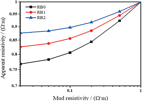
FIGURE 5. Borehole mud correction plate. B0 electrode is the most affected by borehole mud, B2 electrode is the least affected by borehole mud resistivity, and B1 electrode is between the two.

Figure 5 shows that electrode B0 was most affected by the borehole mud, B2 was least affected by the resistivity of the borehole mud, and B1 was in between. This is because, although electrode B0 detects the greatest depth, a large part of the measurement current provided by the electrode flows through the borehole mud to the metal parts on both sides of the pole plate, whereas electrodes B1 and B2, because they are closer to the loop electrode below the pole plate, provide a current that flows back to the loop electrode below through the formation by choosing a closer path, and a smaller proportion of the current flows through the mud to the metal parts on both sides of the pole plate.

4 Optimization of the MCFL tool

To enhance the performance of the MCFL and improve the multiradial depth detection capability of the pole plate, we optimized the focusing method of the instrument. The focusing method of the MCFL designed in this study is based on the digital focusing principle, as shown in Figure 6. The digital focusing method is an advanced method that differs from the traditional hard focusing method, which calculates the focused measurement current by superimposing two independent unfocused measurements. The focusing condition is satisfied by superimposing unfocused measurements to offset supervisory potential. Because the focusing condition is unconditionally satisfied, the effect of the hard focusing feedback monitoring loop on the residual potential is avoided, and the focusing accuracy is improved. In addition, this approach allows for increased flexibility in obtaining different focusing conditions without modifying the hardware. Using the focusing boundary condition (the potential difference between A0 and M is 0):

$U_{A0M}^1+\lambda U_{A0M}^2=0(14)$

Where $U_{A0M}^1$ and $U_{A0M}^2$ denote the potential differences between A0 and M for focus modes 1 and 2, respectively, λ indicating the combination factor.

FIGURE 6

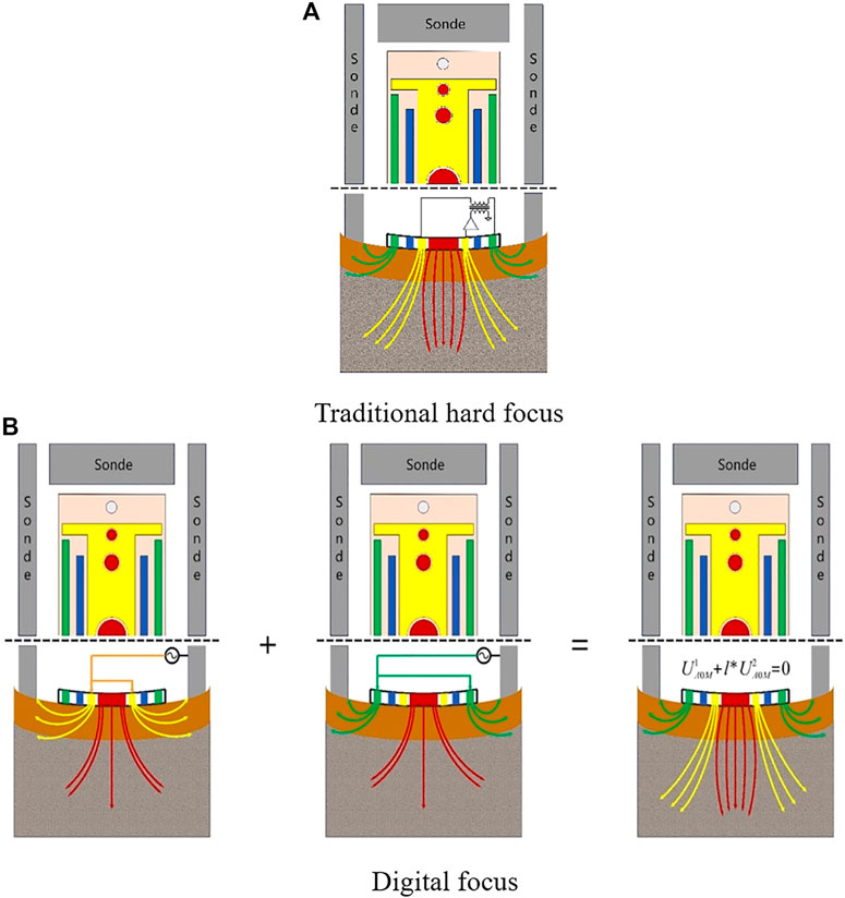
FIGURE 6. Optimization of the MCFL tool. (A) The hard focusing mode. The residual potential of hard focusing mode isn’t equal to 0 in the actual focusing process. The residual voltage cannot be eliminated and the focusing effect is poor. (B)The digital focusing mode. The digital focusing mode can eliminate the influence of residual potential in the actual focusing process and effectively improve the focusing effect of the instrument.

The formula for calculating the apparent resistivity on the three buttons can be obtained:

$R_{Bi}=k_{Bi}\frac{U_{MN}^1+\lambda U_{MN}^2}{I_{Bi}^1+\lambda I_{Bi}^2}(15)$

Where, R_Bi and I_Bi represent the apparent resistivity and current values at different measurement electrodes, respectively. k_Bi represent the scale coefficient of button electrode Bi.

To compare the principle and accuracy of digital focusing circuit, the laboratory physical experiments are carried out in this paper. The physical experiment compares the resistivity results of hard focusing mode and digital focusing mode in three environments of clear water, salt water and distilled water, as shown in Figure 7 and Figure 8.

FIGURE 7

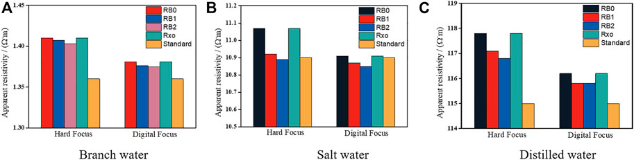
FIGURE 7. Resistivity of aqueous solution with different concentrations for the two focusing methods. (A) The resistivity of the two focusing methods in branch water. (B) The resistivity of the two focusing methods in salt water. (C) The resistivity of the two focusing methods in distilled water. Compared with the traditional hard focus, the resistivity RB0, RB1, RB2, and Rxo measured by digital focus mode in branch water, salt water and distilled water environments are closer to the standard values, and can more restore the formation resistivity. The reason is that digital focusing mode can eliminate the influence of residual potential in the actual focusing process and effectively improve the focusing effect of the instrument.

FIGURE 8

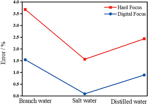
FIGURE 8. Error of aqueous solution with different concentrations for the two focusing methods. Compared with the traditional hard focusing mode, the MCFL using digital focusing has significantly reduced its error, which is 2.14%, 1.45%, and 1.54% lower in the environment of branch water, salt water and distilled water, respectively.

The resistivity measurements of the conventional hard and digital focusing methods in clear water, saltwater, and distilled water environments are shown in Figure 7. It can be observed that both focusing methods can obtain good resistivity measurement results, which are not significantly different from the standard values. In comparison, the digital focusing resistivity measurements of RB0, RB1, RB2, and Rxo in clear water, salt water, and distilled water environments were closer to the standard values and restored the formation resistivity more. The reason is that the digital focusing proposed in this paper can eliminate the influence of residual potential in the actual focusing process and effectively improve the focusing effect of the instrument. Therefore, the effect of the digital focusing resistivity measurements is better than the hard focusing measurements.

The error results of aqueous solutions with different concentrations obtained by the two focusing methods are shown in Figure 8. Compared with the traditional hard focusing method, the MCFL with digital focusing significantly reduced the error by 2.14%, 1.45%, and 1.54% in clear water, saline, and distilled water environments, respectively. In particular, for the saline solution, the digital focusing method controlled the error within 0.09%. The experimental results demonstrate that the micro-cylindrically logging instrument has been optimized by digital focusing, which has greatly improved in performance and can measure the resistivity of the formation with higher accuracy.

5 MCFL data processing and applications

Many inversion methods have been used to interpret log responses, among which gradient-based methods (e.g., the most rapid descent and Gauss–Newton methods) are favored for their ease of implementation and fast convergence (Sun et al., 2008; Kara and Farquharson, 2022). However, in complex inhomogeneous formations, the inversion based on MCFL to determine the formation parameters is non-linear and ill-posed (Shen et al., 2020; Hao et al., 2021). Considering the disadvantages of the gradient-based method, such as huge computation, slow convergence speed in the later iteration stage and extremely sensitive to the selection of initial points, the least square method is used to inverse the measured data in this paper. The advantage of the least square method is that it is simple to calculate and does not require complex gradient calculation, which quickly solve the flushing resistivity, mud cake resistivity and mud cake thickness. On this basis, the micro-normal and micro-inverse curves are synthesized.

5.1 Data inversion method

The relationship between the measured data and stratigraphic parameters is defined as follows:

$\overline{R}=F\left(\overline{g}\right)+\overline{\xi }(16)$

Where, $\overline{R}={\left[RB0,RB1,RB2\right]}^T$, $\overline{g}={\left[Rxo,Hmc,Rmc\right]}^T$, and F are non-linear functions of the formation resistivity response, and $\overline{\xi }$ is the measurement error. The stratigraphic parameters were determined using the least-squares method.

$O=\mathit{min}\left\{‖R-\overline{R}‖\right\}(17)$

Where, $R$ denotes the measurement data vector, $\overline{R}$ denotes the stratigraphic inversion data vector, and O denotes the objective function. The cut-off condition in the inversion process is set as the relative error between the measured value and the forward calculation quantity is less than the preset threshold, that is, the objective function O<10⁻³.

Using the Taylor expansion, the non-linear problem is linearized, and the inverse stratigraphic parameters are obtained from the initial iteration point by gradually iterating the search until O is minimized, $\overline{f}={\left[Rxo,Hmc,Rmc\right]}^T$. The specific process is illustrated in Figure 9. First, the stratigraphic parameters must be initialized, and a response database of different stratigraphic parameters is established. Then, the orthorectified model is used to obtain the logging response characteristics for different formation parameters, and a better solution is found in the logging response database using interpolation fitting, which can quickly approximate the true values of the formation and mudcake parameters being inverted. Because the parameters determined in the database usually don’t satisfy the final required inversion residuals, the above search results must be used as the initial values of the inversion in the next step for the next step of least-squares inversion.

FIGURE 9

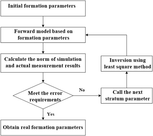
FIGURE 9. Inversion flow chart. The inversion method uses Taylor expansion to linearize the non-linear problem. From the initial iteration point, the iterative search is carried out step by step until the objective function is minimum, and the inversion formation parameters Rxo, Hmc, and Rmc are obtained.

Because the three-button resistivity response curves aren’t at the same depth point, resistivity depth matching is first performed to process the three resistivity curves at the same depth. The inversion processing of stratigraphic parameters was performed using the three original resistivities, and Rxo, Rmc, and Hmc were calculated. Because the resolution of Rxo is the same as that of the original button, resolution matching must be performed to match the resolution of Rxo with a combination of large string instruments to obtain the intrusion zone resistivity curve. The three electrodes on the electrode plate can complete the measurement of two microelectrode curves at the same time. The apparent resistivity of micro-normal and micro-inverse is calculated as follows:

$R_a=K\frac{∆U}{I}(18)$

Where, $R_a$ is the apparent resistivity of micro-normal or micro-inverse. $∆U$ is the measured potential difference of micro-normal and micro-inverse. I is the power supply current intensity. $K$ is the coefficient of micro-normal or micro-inverse electrode system. Figure 10 shows the MCFL data processing flow chart.

FIGURE 10

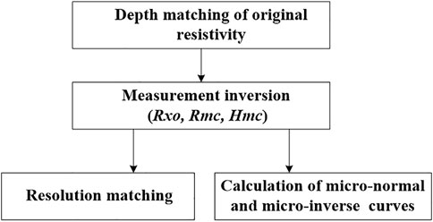
FIGURE 10. Flow chart of data processing of the MCFL. Since the three button resistivity response curves aren’t at the same depth point, it is necessary to carry out resistivity depth matching and resolution matching. Then, the micro-normal and micro-inverse curves are synthesized.

The micro-normal, micro-inverse, and mudcake-thickness response plates are shown in Figure 11. From a set of formation parameters, Rxo, Rmc, and Hmc, two resistivity curves of the micro-normal and micro-inverse can be obtained in real time through forward modeling.

FIGURE 11

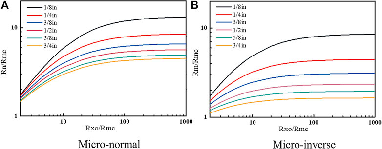
FIGURE 11. Plate of mudcake thickness response. (A) The micro-normal curves. (B) The micro-inverse curves. From a group of formation parameters Rxo, Hmc, and Rmc, two resistivity curves of micro-normal and micro-inverse can be obtained in real time through forward modeling.

5.2 Experiments in the exploration well

When the field needs to use the MCFL tool for logging (as shown in Figure 12), it is first necessary to calibrate the MCFL in the base plant. Its purpose is to establish the correction relationship, mudcake chart and scale coefficient of various influencing factors by calibrating the corresponding relationship between the measured value of the tool and the formation resistivity. The calibration process is as follows: Step 1 is to calibrate the gain and phase offset of each receiving channel. Step 2 is to calibrate the calibration coefficient k of the button electrode in the instrument and convert the accepted electromotive force into the coefficient of apparent conductivity. Step 3 is to use the full resistivity calibration network testing box to externally calibrate the MCFL tool to check the measuring range and accuracy of the MCFL. Then, at the logging site, the logging team uses the inspection device to check whether the MCFL works normally and whether the measured value of the base meets the error requirements. When the instrument is qualified, MCFL can run into the well for measurement.

FIGURE 12

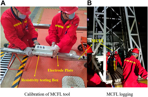
FIGURE 12. MCFL tool calibration and logging operation. (A) Calibration of MCFL tool. Firstly, channel gain, phase and electrode coefficient were calibrated. Then, the measuring range, stability and accuracy of the instrument were tested with a 0.2–2,000 Ω • m network test box. (B) MCFL logging. The well logging team uses the inspection device at the well site to check whether the MCFL tool works normally. Only when the MCFL is qualified can it be put into the well for work.

Figure 13 shows the oil-water layer evaluation map of Well 71 in Ed3 Block of Tianjin Dagang Oilfield. The well section measures nine conventional, array induction, and high-resolution dual lateral curves. Rxo is the resistivity of the intrusion zone obtained from the inversion of the MCFL. This well section is a typical sand-shale with a small amount of siltstone. It can be seen from the figure that in the 2009–2022 m well section, the average porosity is 12.6%. The Rxo resistivity value is significantly lower than the deep and shallow lateral resistivity, which showing low invasion characteristics in the oil layer. In the well section 2032–2042 m, the average porosity is 14.2%. The Rxo resistivity value is significantly higher than the deep and shallow lateral resistivity, which showing a high invasion feature in the water layer. From 2008.1 to 2011 m, the simplified oil test, daily oil production after production 16.7 tons, 1.65 square meters of water, and the water content is 9%.

FIGURE 13

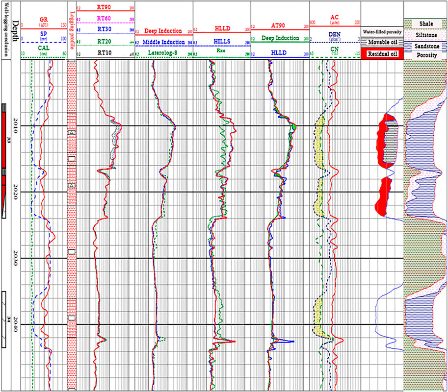
FIGURE 13. The oil-water layer evaluation map of Well 71 in Ed3 Block of Tianjin Dagang Oilfield. This well section is typical sandy mudstone. Rxo in the figure is the resistivity of the invasion charge obtained from the inversion of the MCFL. In the 2009–2022 m well section, Rxo resistivity is significantly lower than the deep and shallow lateral resistivity, which showing low invasion characteristics in the reservoir. In the well section 2032–2042 m, Rxo resistivity is significantly higher than the deep and shallow lateral resistivity, which showing high invasion characteristics in the water layer.

Figure 14 shows the oil-water layer evaluation map of Well 64 in NgⅢ Block of Tianjin Dagang Oilfield. The well section measured nine conventional curves as well as array induction curves. Rmn and Rml in the figure are the micro-normal and micro-inverse curves synthesized by the parameters of MCFL, which the two micro-resistivity curves respond to the permeable layer. This well section is a thin interbed of sand-shale, with a small amount of siltstone mixed in the layer. The average porosity in the layer is about 10%. It can be seen from the figure that at 1979–1990 m and 2011–2012 m, the two micro resistivity curves of the micro-normal and micro-inverse curves are not coincident, which the reactive permeability layer is obvious. From the 2012–2020.14 m in the simplified oil test, the production day is 15.26 tons of oil, 1,230 m³ of gas, 0.34 m³ of water, with a water content of 2.18%.

FIGURE 14

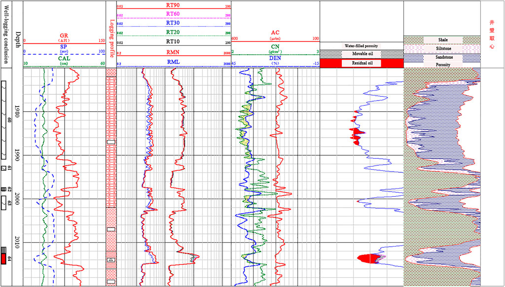
FIGURE 14. The oil-water layer evaluation map of Well 64 in NgⅢ Block of Tianjin Dagang Oilfield. This well section is a thin interbed of sand-shale, with an average porosity of about 10%. At 1979–1990 m and 2011–2012 m, the resistivity value of micro-normal and micro-inverse curves are not coincident, and the reactive permeability layer is obvious.

6 Conclusion

At present, there are few quantitative studies on micro-cylindrically focused logging tool at home and abroad, especially on the problems related to logging in subsurface non-homogeneous media. In this paper, the detection characteristics, stratigraphic correction plates and inversion interpretation of MCFL were investigated using the forward and inverse methods to achieve the purpose of their localization and modification. In addition, to overcome the problem that the residual voltage cannot be eliminated and the focusing effect is poor when the conventional MCFL pole plate is hard focused, the current focusing method of the MCFL was optimized by the digital focusing method, and the measurement accuracy of the MCFL instrument is effectively improved by enhancing the focusing effect of the pole plate. After the verification of the actual logging data, the localized MCFL designed in this paper can successfully replace the foreign-funded tool to achieve the delineation of permeable layers and the identification of oil and water layers (combined with high-resolution dual lateralization).

Data availability statement

The original contributions presented in the study are included in the article/supplementary material, further inquiries can be directed to the corresponding authors.

Author contributions

JX: Project administration, methodology, formal analysis, investigation. ZL: Project administration, formal analysis, methodology, writing—original draft. YJ: Project administration, formal analysis, methodology, writing—original draft. HZ: Investigation, supervision. FL: Methodology, software, investigation. JL: Methodology, formal analysis, supervision. XD: Formal analysis, investigation, writing—original draft and editing.

Funding

The authors acknowledge the financial support by Stable-Support Scientific Project of China Research Institute of Radio wave Propagation (Grant No. A132007W06).

Acknowledgments

We would like to thank Editage (www.editage.cn) for English language editing.

Conflict of interest

HZ was employed by CNOOC Limited.

The remaining authors declare that the research was conducted in the absence of any commercial or financial relationships that could be construed as a potential conflict of interest.

Publisher’s note

All claims expressed in this article are solely those of the authors and do not necessarily represent those of their affiliated organizations, or those of the publisher, the editors and the reviewers. Any product that may be evaluated in this article, or claim that may be made by its manufacturer, is not guaranteed or endorsed by the publisher.

References

Bai, Y., Yang, S., Ma, Y., Chen, T., Guo, Y., and Wang, H. (2018). Adaptive borehole correction of three-dimensional array induction logging data in a vertical borehole. Chin. J. Geophys. 61 (9), 3876–3888. doi:10.6038/cjg2018L0082

CrossRef Full Text | Google Scholar

Chen, X., and Nie, Z. (1997). Numerical solution of microlaterolog devices by 3D finite element method in inhomogeneous media. Comput. Tech. Geophys. Geochem. Explor 19 (3), 11–18. doi:10.3969/j.issn.1001-1749.1997.03.02

CrossRef Full Text | Google Scholar

Deng, S., Li, Z., and Chen, H. (2010). The simulation and analysis of array lateral log response of fracture in coalbed methane reservoir. Coal Geol. Explor. 38 (3), 55–58. doi:10.3969/j.issn.1001-1986.2010.03.013

CrossRef Full Text | Google Scholar

Donadille, J. M., Ilyin, I., Luling, M., Meszaros, T., Reischman, R., Repnev, A., et al. (2017). “Slim, high resolution laterolog array tool: First field experiences,” in Proceeding of the SPE/AAPG/SEG Unconventional Resources Technology Conference, Austin, USA, July 2017, 1645–1657. doi:10.15530/URTEC-2017-2671192

CrossRef Full Text | Google Scholar

Gao, J., Sun, J., Jiang, Y., Zhang, P., and Wu, J. (2017). Weighted processing for microresistivity imaging logging in oil-based mud using a support vector regression model. Geophysics 82 (6), D341–D351. doi:10.1190/geo2016-0592.1

CrossRef Full Text | Google Scholar

Guo, Q., He, F., He, L., Yang, J., Cao, J., You, Z., et al. (2021). Theory and algorithm research on the ratio of main current&bucking current and rest potential circuit measurement of laterolog tool. Electron. Meas. Technol. 44 (5), 81–83. doi:10.19651/j.cnki.emt.2005454

CrossRef Full Text | Google Scholar

Hao, P., and Sun, X. (2017). “Investigation and analysis of focusing ability and instrument structures of micro-cylindrically focused logging,” in Proceeding of the 2017 Sixth Asia-Pacific Conference on Antennas and Propagation-APCAP, Xi’an, China, October 2017, 1–3.

CrossRef Full Text | Google Scholar

Hao, P., Sun, X., and Nie, Z. (2018). “Influence of different formation parameters on electromagnetic response of micro-cylindrically focused logging,” in Proceeding of the 2018 IEEE International Geoscience and Remote Sensing Symposium- IGARSS, Valencia, Spain, July 2018 (IEEE), 1308–1311. doi:10.1109/IGARSS.2018.8518254

CrossRef Full Text | Google Scholar

Hao, P., Zhao, Y., Sun, X., and Nie, Z. (2021). “Robust inversion scheme for logging responses interpretation of micro-cylindrically focused logging,” in Proceeding of the 2021 IEEE International Geoscience and Remote Sensing Symposium-IGARSS, Brussels, Belgium, July 2021 (IEEE), 2951–2954. doi:10.1109/IGARSS47720.2021.9553310

CrossRef Full Text | Google Scholar

Jin, J. (1998). “3D finite element analysis,” in Finite element method of electromagnetic field (Xi’an: Xidian University Press), 96–102.

Google Scholar

Kara, K. B., and Farquharson, C. G. (2022). 3D minimum-structure inversion of controlled-source EM data using unstructured grids. J. Appl. Geophysi. 209, 104897–104912. doi:10.1016/j.jappgeo.2022.104897

CrossRef Full Text | Google Scholar

Li, Z., Fan, Y., Deng, S., Ji, X., and Li, H. (2010). Inversion of array laterolog by improved difference evolution. J. JinLin Univ. (Earth Sci. Ed. 40 (5), 1199–1204. doi:10.3969/j.issn.1671-5888.2010.05.034

CrossRef Full Text | Google Scholar

Li, H., Fan, Y., Hu, Y., and Deng, S. (2012). Five-parameter inversion method of array induction logging. J.China. Univ. Pet. (Ed. Nat. Sci.) 36 (6), 47–52+61. doi:10.3969/j.issn.1673-5005.2012.06.008

CrossRef Full Text | Google Scholar

Li, Z., Yang, L., Yao, W., Xia, J., and Zhang, K. (2017). Numerical simulation and application of micro-cylindrically focused logging responses. Well Logging Technol. 41 (3), 310–314. doi:10.16489/j.issn.1004-1338.2017.03.012

CrossRef Full Text | Google Scholar

Merchant, G., Maurer, H., and Zhou, Z. (2006). “Estimation of flushed zone and mudcake parameters using a new micro-resistivity pad device,” in SPWLA 47th Annual Logging Symposium (Veracruz, Mexico: OnePetro).

Google Scholar

Ren, T., Feng, B., Sun, W., Zhang, C., and Tang, D. (2021). Multi-objective optimization design of push system for microsphere focusing logging tool. J. Southwest Pet. Univ. Sci. Tech. Ed. 43 (1), 157–166. doi:10.11885/j.issn.1674-5086.2018.08.01.01

CrossRef Full Text | Google Scholar

Salazar, J. M., and Torres-Verdín, C. (2009). Quantitative comparison of processes of oil-and water-based mud-filtrate invasion and corresponding effects on borehole resistivity measurements. Geophysics 74 (1), E57–E73. doi:10.1190/1.3033214

CrossRef Full Text | Google Scholar

Shen, Q., Chen, J., Wu, X., Han, Z., and Huang, Y. (2020). Parallel tempered trans-dimensional Bayesian inference for the inversion of ultra-deep directional logging-while-drilling resistivity measurements. J. Pet. Sci. Eng. 188, 106961–106911. doi:10.1016/j.petrol.2020.106961

CrossRef Full Text | Google Scholar

Sun, X., Nie, Z., Li, A., and Luo, X. (2008). Analysis and correction of borehole effect on the responses of multicomponent induction logging tools. Prog. Elect. Res. 85, 211–226. doi:10.2528/PIER08072206

CrossRef Full Text | Google Scholar

Tian, Z., Yan, W., and Qin, K. (2003). On variations of formation resistivity in fresh drilling mud invasion. Well Logging Technol. 27 (2), 113–117+177. doi:10.16489/j.issn.1004-1338.2003.02.006

CrossRef Full Text | Google Scholar

Wang, H. (2003). Simultaneous reconstruction of geometric parameter and resistivity around borehole in horizontally stratified formation from multiarray induction logging data. IEEE Trans. Geosci. Remote Sens. 41, 81–89. doi:10.1109/TGRS.2002.808070

CrossRef Full Text | Google Scholar

Wang, Y., and Wu, X. (1994). On K value of MSFL tool for heterogeneous media. Well Logging Technol. 18 (1), 22–25. doi:10.3969/j.issn.1004-1338.1994.01.004

CrossRef Full Text | Google Scholar

Wu, Z., Yue, X., Li, G., Liu, T., and Zhao, J. (2022). A novel and efficient dimensionality-adaptive scheme for logging-while-drilling electromagnetic measurements modeling. J. Pet. Sci. Eng. 215, 110572–110581. doi:10.1016/j.petrol.2022.110572

CrossRef Full Text | Google Scholar

Xia, J., Gao, C., Li, Z., Zhang, J., and Feng, Y. (2015). Design and application of micro-cylindrical resistivity and three-detector lithology density combined logging tool. Pet. tubu. Goods Instr. 1 (4), 11–14. doi:10.3969/j.issn.1004-9134.2015.04.004

CrossRef Full Text | Google Scholar

Xing, G., Xu, H., and Teixeira, F. L. (2018). Evaluation of eccentered electrode-type resistivity logging in anisotropic geological formations with a matrix method. IEEE Trans. Geosci. Remote Sens. 56 (7), 3895–3902. doi:10.1109/TGRS.2018.2815738

CrossRef Full Text | Google Scholar

Zeng, C., Zhang, Y., Li, Y., Peng, Y., Wang, Y., Zhao, J., et al. (2010). Synthesis of microelectrode curves using microspherical focused logging data. J. Yangtze Univ. Nat. Sci. Ed. 7 (1), 275–277. doi:10.16772/j.cnki.1673-1409.2010.01.025

CrossRef Full Text | Google Scholar

Zhao, P., Qin, R., Pan, H., Ostadhassan, M., and Wu, Y. (2019). Study on array laterolog response simulation and mud-filtrate invasion correction. Adv. Geo-Energy Res. 3 (2), 175–186. doi:10.26804/ager.2019.02.07

CrossRef Full Text | Google Scholar

Zhou, F., Meng, Q., Hu, X., Slob, E., Pan, H., and Ma, H. (2016). Evaluation of reservoir permeability using array induction logging. Chin. J. Geophys. 59 (6), 703–716. doi:10.1002/cjg2.30018

CrossRef Full Text | Google Scholar

Zhou, T. (2003). Micro-cylindrically focused logging tool. J. Oil Gas. Technol. 25 (S1), 36–37+5. doi:10.3969/j.issn.1000-9752.2003.z1.018

CrossRef Full Text | Google Scholar

Zhu, P., Li, Z., Chen, M., and Dong, Y. (2019). Study on forward and inversion modeling of array laterolog logging in a horizontal/highly deviated well. Acta geophys. 67 (5), 1307–1318. doi:10.1007/s11600-019-00321-2

CrossRef Full Text | Google Scholar