K-span: Open and reproducible spatial analytics using scientific workflows

1 Introduction

Reproducible research encourages scientists to publish not only their findings, but also the data, code, and software used to produce those findings (Peng, 2011; Cohen-Boulakia et al., 2017; Kitzes et al., 2018). By enabling others to interrogate any aspect of an analytics process, scientific research becomes far more transparent and verifiable. There are two major barriers to implementing reproducible research: making the data used available and making the analytics process accessible. Of the two, making the data available has seen the most progress, led by the open data movement, which encourages not only scientists but also governments and industry to publish the data they generate in an accessible, non-proprietary format (exemplified by the FAIR—findable, accessible, interoperable, and reusable—data movement Wilkinson et al., 2016, for instance).

While making the code and data used to produce research available does greatly improve reproducibility, sharing code alone may not be reproducible by those without the necessary technical expertise or if it relies on proprietary software (Kitzes et al., 2018; Radosevic et al., 2020). In addition to producing results that may be in a proprietary and closed format, the code of proprietary software is generally not available for review, usually resulting in an aspect of the process that cannot be interrogated. Open source software (OSS) addresses this issue by making the code freely available for anyone to use, analyze, and modify. OSS is used extensively in the field of geospatial science, with software such as GDAL¹, QGIS², and PostGIS³ being used to develop solutions for geospatial processes in areas such as environmental modeling (Callaghan et al., 2010; Neteler et al., 2012; Thorp and Bronson, 2013; Turuncoglu et al., 2013), hydrological modeling (Horsburgh et al., 2015; Leonard and Duffy, 2016; Sangireddy et al., 2016), and drainage systems (Riaño-Briceño et al., 2016).

The increasing availability of open spatial data and diversity of open spatial software presents both opportunities and challenges. The ubiquity of spatial data and tools today is helping to seed new hypotheses in diverse areas of science and to reveal new patterns in big data. On the other hand, the computational and conceptual complexity of many spatial data analytics procedures presents significant challenges to the efficiency and reproducibility of those analytics.

In this paper we explore the design, development, and testing of an open and reproducible KNIME spatial analytics workflow tool (called “K-span”), based on existing open-source spatial tools combined with a general-purpose scientific workflow platform. We chose KNIME⁴ (Konstanz Information Miner) (Berthold et al., 2009; Warr, 2012) as our open-source scientific workflow platform (discussed further in later sections). The K-span integrates a range of common open-source spatial tools and formats, including GeoTools, GDAL, PostGIS, and GeoJSON with existing KNIME capabilities as a freely available, open-source KNIME spatial analytics workflow tool. The benefits of the K-span software tool include:

• Openness: Scientific workflows help to decompose complex spatial analytics processes into a sequence of unambiguous spatial operations connected by data flows (Bakos, 2013; Liew et al., 2016). Managing complexity in this way makes it easier for anyone to create, adapt, remix, reuse, and reproduce spatial analytics. The approach also makes it easier to integrate non-spatial operations, such as machine learning and data mining techniques, not common in today’s siloed GIS tools (Morisette et al., 2013; Radosevic et al., 2020). Reliance on open-source tools further decreases dependency on proprietary software and increases the options for openness and reproducible spatial analysis.

• Transparency: The diversity of spatial operations (e.g., distance may refer to Euclidean, Manhattan, or Hausdorff measures) and even implementations of those operations (e.g., both the winding number and crossing number algorithms can be used to determine if a point is inside a polygon) frequently leads to bespoke or poorly documented steps in spatial analytics today. Scientific workflows make implicit decisions explicit. Together with open data, scientific workflows can turn spatial analytics into “executable documentation,” giving industry and government certainty about how exactly data was created and decisions were made (Ludäscher et al., 2009).

• Automation: By providing a visual language for spatial analytics, spatial workflows can automate data analysis and enable a more user-friendly approach than programming, but more rigorous and reproducible than ad hoc use of menu-driven desktop tools, such as GIS (Yue et al., 2015; Yin et al., 2018). This combination provides and ideal environment for integrated and collaborative prototyping and development of automated spatial analytics.

In this context, the key contributions of this paper are:

1 The building and implementation of the open-source K-span software tool built on the freely available KNIME scientific workflow platform. The result provides a visual language for spatial analytics, allowing users to combine geospatial analysis with other data analytics techniques for efficient processing of large geospatial datasets.

2 The application of the spatial scientific-workflow approach to a major case-study of constructing the national Digital Elevation Model (DEM) for Geoscience Australia⁵ (GA) (Geoscience Australia, 2015). The result is a more open, transparent, automated, and reproducible procedure for building a foundational spatial dataset of national significance.

3 A qualitative and quantitative evaluation of the differences between the conventional (“black box”) approach to constructing a DEM and our open and reproducible scientific-workflow approach. The potential for increased assurance and confidence in spatial data products—sometimes termed “warrantability”—using our approach is a key finding of our results.

The rest of this paper is organized as follows. Section 2 provides further background into the scientific workflows approach to spatial analytics. The design and development of the K-span software tool is described in Section 3. Section 4 presents our reference case study for building a K-span workflow for DEM construction and Section 5 describes the results through qualitative and quantitative comparisons with GA’s prior DEM construction process. Finally, Section 6 concludes the paper with a discussion of future work.

2 The scientific workflows approach

This work seeks to combine the benefits of reproducible research, open data, and open source software to create an open, transparent and automated computational tool for constructing spatial analytics. To do so, we make use of scientific workflows. While workflow-based technologies were first adopted by the business community, they have drawn a great deal of attention in the databases and information systems research and development communities (Barker and Van Hemert, 2007). Like business workflows, scientific workflows are executable models constructed through intuitive and interactive graphical user interfaces. Scientific workflows apply the workflow paradigm for describing, managing, and sharing solutions to complex scientific problems. They commonly adopt a dataflow-oriented approach, where a complicated analytics task can be modularized into chains of analysis operations connected by data flows.

In the past scientific workflow systems were used extensively in the field of bioinformatics to not only capture analytical processes but also to document those processes amongst collaborators for review and revision (Sun et al., 2011). While scientific workflows are used extensively for non-spatial processes (Brown et al., 2007; Barseghian et al., 2010), their ability to conduct spatial operations are still in the initial stage of development (Callaghan et al., 2010; McFerren et al., 2012; Zyl et al., 2012; Yue et al., 2015; Scheider and Ballatore, 2017; Radosevic et al., 2020). Some researchers have already propounded the use of scientific workflows for spatial analytics (Ludäscher et al., 2006; Freire et al., 2018; Kitzes et al., 2018; Radosevic et al., 2020; Cerutti et al., 2021). These workflows allow users to break down complex spatial analytics tasks into chains of modular components (Zhang et al., 2006; Zyl et al., 2012; Yue et al., 2015).

One example is the Kepler⁶ scientific workflow system, which has made progress developing nodes for spatial operations (Jaeger et al., 2005). The platform is becoming increasingly capable of processing large amounts of spatial data such as point clouds produced from Light Detection and Ranging⁷ (LiDAR) data (Crawl and Altintas, 2008). To aid in processing large amounts of data, cluster capabilities have been added to Kepler (Ludäscher et al., 2006), along with parallel processing capabilities using mapReduce (Wang et al., 2012).

Of the scientific workflow platforms under active development, we found that Kepler, KNIME, VisTrails⁸, and Apache Taverna⁹ (Hull et al., 2006) met our requirements of being OSS, cross-platform, scalable from a single desktop to high performance computing environments, containing a wide variety of inbuilt non-spatial analytics, and ease of incorporating spatial operations.

2.1 KNIME

KNIME is written in Java and comes with an extension mechanism to simplify the process of adding plugins for providing additional functionality. This has allowed a large number of community contributors to create their own plugins, in addition to the wide range of integrated tools such as machine learning algorithms from Weka and the statistics package R.

We ultimately chose KNIME over the other options primarily due to its ability to selectively execute each node within a workflow. This is in contrast to the other platforms investigated, which require the entire workflow to be executed. Specifically, when a node is executed in KNIME, only that node, and any unexecuted dependent nodes (i.e., its descendant nodes) will run. While all scientific workflow platforms are capable of decomposing a complex spatial process into a set of discrete steps (i.e., nodes), KNIME allows for each step to be individually executed, with its results, models, and interactive views available for inspection and alteration at any time.

KNIME utilizes a table-based approach to data representation, where data attributes are stored as columns and data instances are stored as rows. Figure 1 shows an example workflow including our implemented nodes in the KNIME workbench, where squares represent processes applied to the data and arrows represent the flow of data. Specifically, a KNIME data processing node will have some or all of the following components.

1 A set of input ports used for taking input data in tabular format.

2 A node dialogue for configuring processing parameters (e.g., to set the distance for a buffer operation).

3 A set of output ports to represent the results of the process in tabular format.

4 A result visualizer to graphically display information about the process’ output (e.g., a map, graph, or image).

FIGURE 1

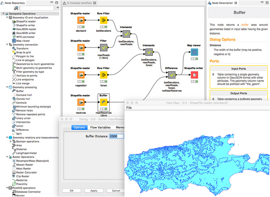
FIGURE 1. An overview of our implemented nodes in the KNIME workbench. The node repository panel (left) presents our developed spatial nodes (Geometry IO and visualization, Geometry conversion, Geometry processing, Geometry relations and measurements, Raster operations and PostGIS operations—for the full list of nodes in the K-span software tool see Table 1), a configuration window (bottom left) shows options available for the buffer node, spatial data is displayed by the map viewer node in a map window (bottom right), and detailed documentation about the node is presented in the right panel.

Not all OSS that are capable of spatial analytics make use of scientific workflows. QGIS, a popular open source GIS software, does have some scientific workflow capabilities (Cagnacci and Urbano, 2008), utilizing a built-in graphical modeler to construct workflows. Nevertheless, its workflow interface is tailored towards constructing simple spatial analytics workflows for use in batch processing, and as such does not scale well to large, complex and automated scientific workflows built with KNIME. The focus of QGIS is not directed towards documentation of spatial analytics process, but rather to enable visualization of spatial data using manually executed processes. In contrast, KNIME is capable of providing detailed documentation and annotation of the whole spatial analytics process. Such limitations are a natural consequence of QGIS being a GIS with added workflow capabilities rather than software designed as a workflow system from the ground up, such as KNIME.

Further, most other open source data analysis tools are limited by significant working memory constraints whereas KNIME is a scalable workflow platform capable of processing very large data volumes without restrictions on RAM or working memory Berthold et al. (2009). The K-span software tool can therefore take advantage of some of KNIME’s general features including memory management, which allows scaling to billions of rows with a desktop computer. This feature is vital for our DEM case study, given that we need to process terabytes of data. KNIME workflow models are stored in plain-text XML files, making them human-readable and easy to parse. The models can also be easily exchanged with or without data. Moreover, KNIME allows wrappers for calling other code in addition to providing nodes that allow to run R, Python, Perl, and other code fragments.

3 K-span software tool

To integrate geospatial operations and processing, we developed K-span, a KNIME software tool containing various spatial analytics nodes for working with geospatial data. The K-span software tool was designed to take advantage of existing OSS libraries, integrating them to fulfill our needs, in preference to reimplementing fundamental spatial operations (such as GIS overlay, buffer, controid, and topological operations on geometries). Specifically, we reuse established spatial algorithms in existing libraries and expose that functionality in KNIME by building a new K-span node with appropriate input and output ports based on that process’ structure and purpose. By adopting this component-based approach, we simplify the development process and provide control over modularity.

For example, to process vector-based spatial data we make use of GeoTools, an open-source Java library that provides methods for the manipulation of geospatial data. By providing the basic components of spatial data processing, GeoTools allows developers to focus on higher-level geospatial processes by re-using basic functions such as reading a Shapefile, buffering a geometry, or styling and displaying a set of features. GeoTools also provides interfaces for spatial concepts and data structures, and is itself built on open-source libraries such as the JTS¹⁰ (Java Topology Suite) and Open Geospatial Consortium’s (OGC) GeoAPI¹¹. JTS provides a complete, consistent, and robust implementation of fundamental algorithms for processing linear geometry on the 2-dimensional Cartesian plane, and supports modeling geometry as points, linestrings, polygons, and geometry collections (Shekhar and Xiong, 2008).

Given that such representations do not fit neatly into a table-based structure, however, K-span required a suitable tabular data format rapidly interchangeable with the geometry and ideally human-readable. Accordingly, we adopted the GeoJSON¹² format, capable of encoding a variety of geographic data structures in a human readable text-based format, along with their non-spatial attributes (Butler et al., 2016). GeoJSON is based on JavaScript Object Notation¹³ (JSON), and is an open and widely used format. Since we need to store vector geometries in a format compatible with KNIME tables, we take advantage of GeoTools’ GeoJSON library to store the spatial aspect of data. Specifically, geometries and their coordinate reference systems are stored as GeoJSON strings in a geometry column, with the non-spatial data stored alongside in separate columns of the table. Table 1 presents the list of geospatial data processing nodes we have developed to date. Nodes are grouped in eight different categories, and each node is constructed to serve a specific spatial operation. In addition, each node includes a dialog pane¹⁴ (see Figure 2 for an example of node dialog pane) enabling openness and transparency of the K-span software tool by allowing users to reuse, edit, adapt and modified the node settings. Following sections go further into details about each node category.

TABLE 1

TABLE 1. Developed and implemented the K-span software tool to KNIME.

FIGURE 2

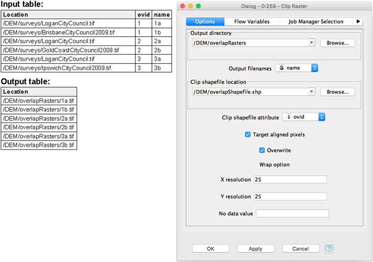
FIGURE 2. Example of the Clip raster node in operation, with input table and output tables on the left, and node dialogue pane on the right.

3.1 Geometry input output (IO) and visualization nodes

This category of workflow nodes read or write data and are used for the import, export, or display of geospatial data. Import nodes such as the Shapefile and GeoJSON readers make use of node dialogue panes to identify file locations. Next, these nodes read the input file’s data and convert input data geometry along with other non-spatial attributes to a table format for easier manipulation by other nodes. For example, the Shapefile reader¹⁵ reads an ESRI Shapefile¹⁶ and creates an output data table which includes geometries (polygon, line, or point) and other non-spatial information in the Shapefile. Such “reader nodes” are unusual in that they have only an output port, reading the input data from a specified location on file (cf. Figure 1). “Writer” and “viewer” nodes, in contrast, lack an output port taking in a geometry table through their input port. “Writer” workflow nodes store input geometry along with its associated non-spatial attributes in a location specified using the node dialogue pane. For instance, the Shapefile writer¹⁷ stores the input data table in an ESRI Shapefile specified by a destination location. The Map viewer workflow node works similarly to generate a simple map view of the geometries, allowing the user to quickly view the geometry without having to export and load the data into another system (see Figure 1).

3.2 Geometry conversion nodes

Geometry conversion workflow nodes convert geometries from one type to another while the underlying vertices remain in the same location. These workflow nodes are unary (take a single input), transforming each geometry in a column of input geometries into a corresponding geometry in an output geometry column. For example, the Transform node applies changes to geometry of selected geometric features listed in input table by using displacement vectors or spatial reference IDs (SRID) to enable the best-fit geometric transformation between two different coordinate systems (ESRI, 2021). Nodes in this category possess both input and output ports. An spatial input table requires a geometry column in GeoJSON format. The output table contains a second, additional output geometry column in GeoJSON format. In many cases, parameters are not required for geometry conversion and so the workflow node does not contain a dialogue pane. Where parameters are required, (e.g., a new coordinate reference system for the transform node or a grid size for the snap to grid node), they are captured via the workflow node dialogue pane. In either case, all nodes validate inputs before execution and highlight potential errors. For example, the Polygons to lines geometry conversion node will warn the user if the input table does not contain any polygons or multi-polygons.

Almost all workflow nodes in this category exhibit a one-to-one relationship between the rows of the input and output Tables. A few, such as Geometries to multi-geometriesi exhibit a one-to-many relationship, taking rows with a geometry collection or a multi-point, line, or polygon and splitting out individual geometries to their own row. Each output row contains a copy of any non-spatial data associated with the original row. Multi-geometries to geometries is the opposite of this, exhibiting a many-to-one relationship and taking rows and combining them into a single row as either a geometry collection, or a multi-point, line, or polygon.

3.3 Geometry processing nodes

Geometry processing nodes take input geometries and process them into new geometries, potentially altering their underlying vertices. For example, the Buffer¹⁸ node creates a new geometry with a buffered area based on a supplied distance around geometries in the input table. While most processing workflow nodes are unary in their input, some are binary. For example, overlay spatial operations executed with Intersection, Union, Difference, and Split workflow nodes require two sets of geometries. Specifically, these workflow nodes take the first two geometry columns from the input table and produce a single output geometry column. All geometry processing workflow nodes exhibit a one-to-one relationship between the rows of the input and output tables and simply pass through all non-spatial columns.

3.4 Geometry relations and measurements nodes

While workflow nodes from the previous two categories output altered geometries from the geometries passed through to them, workflow nodes in this category take in geometries and pass out non-spatial data. For example, the Area workflow node takes in a single column of polygons, multi-polygons, or geometry collections and determines the total area for each row. All workflow nodes in this category pass through the original geometries and non-spatial columns unaltered and require no input parameters. Some workflow nodes, such as Distance and the Boolean operations, are binary in their input and require two geometry columns. All table columns are passed through unaltered. Lastly, some workflow nodes exhibit polymorphism, meaning that they use different processing algorithms depending on the input data. For example, if the Length/perimeter workflow node takes in lines or multi-lines, it will output a length whereas it will output a perimeter for geometries (polygons) or multi-geometries.

3.5 Raster operations nodes

Raster operations nodes apply spatial operations for preparing, manipulating, and analyzing raster data. Given that our reference case study (see Section 4) involves the processing of massive volumes of raster data, a robust and efficient raster processing library was required. In light of this, we have built the K-span raster processing nodes on GDAL, the Geospatial Data Abstraction Library (Warmerdam, 2008). GDAL is equipped with a variety of useful command line utilities for translating and processing raster and vector data stored in a variety of formats.

Raster files tend to be very large and stored in a variety of formats. Hence, it is not practical to directly pass raster data through KNIME workflow nodes in tabular format. Instead, only information about the raster files’ location on a local disk or a remote server is passed to the workflow nodes. In particular, our Raster operations workflow nodes require the following three components to process raster images.

1 A location column in the input table, which stores the complete path to the raster.

2 An output directory in the node dialogue window (see Figure 2), which allows the user to indicate the folder the output rasters are stored in.

3 An output name selector in the node dialogue window, which allows the user to select a column in the input table with the required names of the output rasters.

By making use of raster file locations, large sets of rasters can be processed simultaneously. Figure 2 shows an example of the Clip raster node in configuration, taking in various raster files and clipping them to the boundaries of a Shapefile. By ensuring that the output of any raster node includes a location column, raster operations can be chained together in a similar way to the vector operations. Raster images can either be viewed within KNIME using the Image viewer workflow node (Dietz and Berthold, 2016) or can be accessed by an external application such as QGIS.

3.6 PostGIS operations nodes

PostGIS operations nodes were implemented to facilitate processing of remotely-located spatial data. While some workflow nodes such as the Raster operations workflow nodes and the Web Feature Service (WFS)¹⁹ connector workflow node are capable of retrieving spatial data from remote locations, all of the workflow nodes discussed so far have been limited to processing data locally.

Some existing KNIME workflow nodes (PostgreSQL, Secure Socket Shell, etc.) are also capable of processing data remotely. These KNIME nodes are not specifically designed with spatial processes in mind, however. To make use of PostGIS (Obe and Hsu, 2015), we developed an extension to the standard KNIME PostgreSQL workflow nodes that supports geographic objects. Our extension allows the connection to a PostGIS database to read or write geometries in tabular format. Figure 3 shows an example workflow in KNIME using our PostGIS operations workflow nodes where database queries are written using the workflow node dialogue pane. As an open and transparent software tool, the K-span allows users to write new or inspect and reuse the existing queries within Reader workflow node settings. In addition, results can be displayed using the Map viewer workflow node.

FIGURE 3

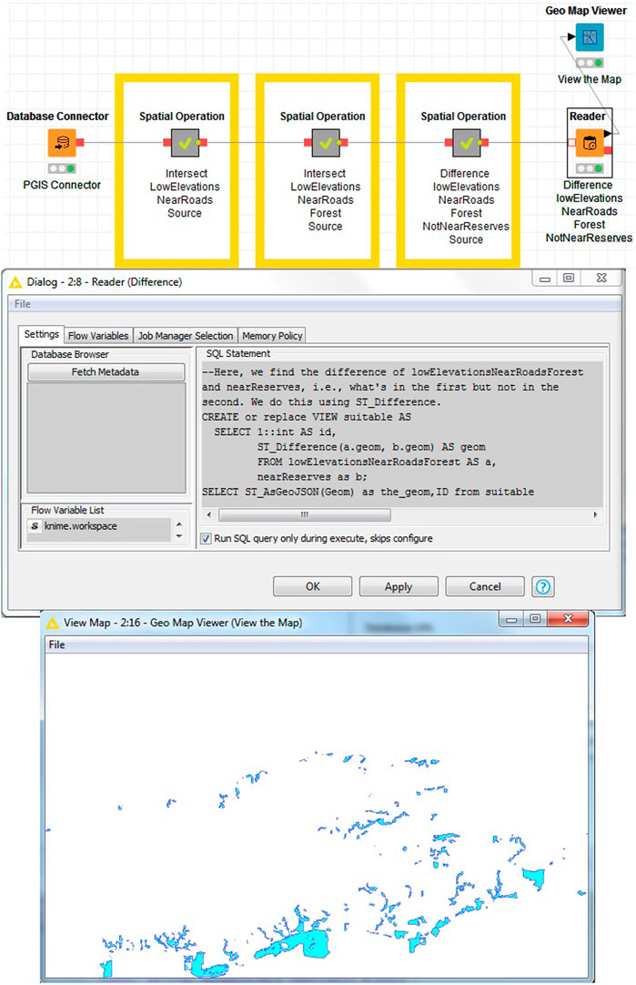
FIGURE 3. Example of a workflow in KNIME executing spatial processes remotely using PostGIS operation nodes.

3.7 Metanodes

A group of connected workflow nodes that performs some useful task can combined into a single node, called a “metanode.” Metanodes enable complex configurations of nodes to be collapsed into a single node for clarity and modularity. An example of a metanode for a intersection operation is shown in Figure 4. Metanodes can themselves be nested, further facilitating both the readability and modularity of a workflow by describing processes at multiple levels of granularity. K-span includes two metanodes: Intersects and Difference for performing intersection and difference between geometries.

FIGURE 4

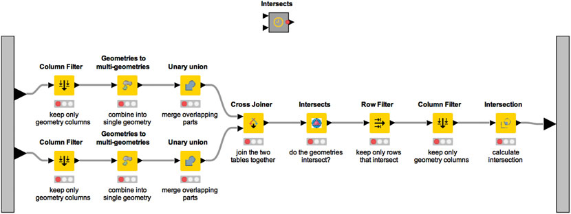
FIGURE 4. Example of an Intersects workflow metanode. This metanode takes in two tables and removes their non-spatial columns before collapsing the geometry into a single row. The two tables are then joined, and checked to see if they intersect before the intersection operation is performed. A single data table with intersected geometry is then output.

3.8 Custom code integration node

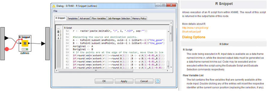
Finally, KNIME also supports the ability to integrate snippets of code from a variety of languages within workflow nodes. While not part of the K-span software tool, the case study in the next section makes limited use of the R snippet workflow node, integrating R code for spatial analysis into the workflow. Figure 5 shows an example of such a workflow node used in our case study, which calculates the least cost shortest path through a raster image between two points, and highlights the flexibility to integrate an enormous range of different tools, libraries, and software into a single workflow.

FIGURE 5

FIGURE 5. Example of R snippet workflow node with custom code integration.

4 SCDEM workflow

The main aim of our work is to develop a more open, transparent, automated, scalable, and reproducible spatial analytics software tool. Hence, it is important that any software tool developed is not just made available, but is also self-documented and modifiable by interested user or institution. At present, GA, a government institution uses ESRI’s ArcGIS for a process of constructing national DEM. ESRI’s ArcGIS is a GIS proprietary software that is not freely available for users to create, analyze and manage spatial analytics. While it would be possible to reimplement the process by using a proprietary (“black box”) workflow systems that are capable of geospatial processing, such as ESRI’s ModelBuilder²⁰ (a workflow tool available within ESRI’s ArcGIS), this would not meet our requirements for openness and reproduction of spatial analytics. The main aim of ESRI’s ModelBuilder is not focused on documentation of spatial analytics, but rather to enable graphical representation of spatial data using manually executed processes. In particular, ArcGIS is a proprietary GIS software with added workflow capabilities rather than a scientific workflow system, such as KNIME. Feature Manipulation Engine²¹ is another proprietary and not freely available spatial analytics workflow tool for managing and executing data driven processes. Nevertheless, application of these “black box” software tools would still not meet our requirements of openness, transparency and documentation. Hence, we applied, tested and validated our K-span software tool by building and implementing a SCDEM workflow which overcomes the limitations of the original GA process.

4.1 Case study

Our K-span software tool was applied, tested and validated on a key part of the process used by GA to construct the national Australian DEM of Greater Brisbane, and a component of the national Australian Foundational Spatial Data Framework²² (FSDF).

The process chosen involves constructing a seamless coastal Digital Elevation Model (SCDEM) from individual LiDAR height surveys. The SCDEM process was documented, with a written operator’s manual explaining the process in detail. A breakdown of the 11 steps of the original SCDEM construction process is shown in Figure 6.

FIGURE 6

FIGURE 6. 11 steps of the original SCDEM construction process.

Figure 7 shows the sample study area chosen for this work, comprising 13 LiDAR surveys centered on Brisbane and covering an area of approximately 18,000 km². The figure highlights the 23 areas of overlap between the 13 individual surveys.

FIGURE 7

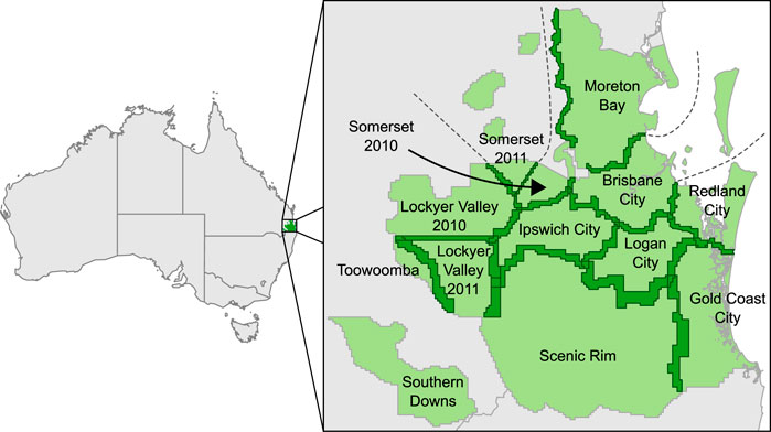
FIGURE 7. Outlines of the 13 surveys (light green), used in our Greater Brisbane, Australia, case study, with overlaps in dark green.

4.2 The workflow design and implementation

Our workflow implementation of the SCDEM construction process is a new reproducible scientific workflows approach for generating the national DEM. It is an open, transparent, automated and improved version of the original GA process. The SCDEM workflow also represents an “executable documentation” supported with our K-span open source and freely available software tool while replacing ESRI’s ArcGIS proprietary (“black box”) software tool as the spatial analytics engine. In particular, our workflow is capable to execute and reproduce the 11 main steps of the original SCDEM process showed in Figure 7. Also, in our workflow, the SCDEM process was built and implemented to be fully automated and to run without user intervention. A summary of the SDEM workflow is shown in Figure 8, with one of the metanodes (Step 4, Calculate cutline endpoints) expanded by two levels to show further detail. The workflow was mainly built from the K-span nodes described in Section 3 and some of existing nodes within KNIME.

FIGURE 8

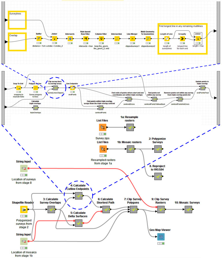
FIGURE 8. The SCDEM workflow for executing the original GA process. At the bottom is the overall metanode steps and data flow (cf. Figure 6). The middle part shows the expanded metanode for one step (Step 4, Calculate cutline endpoints). At the top is the further expansion of one step in Step 4.

The building and implementation of the SCDEM workflow involved the following 10 main steps:

1 Resample and Mosaic surveys: In the first step our workflow reads and ranks LiDAR surveys based on their age (newer to older). Each survey contains a set of raster tiles. These tiles are resampled with Resample/warp/reproject workflow node to a specific resolution (25 × 25 m) and named sequentially in order to place each tile in its own rank folder. The purpose of this data management process is to avoid duplicate tile filenames. After that each survey and every resampled tile within that survey is selected and joined into a single image mosaic using Mosaic raster spatial analytics workflow node and given its name according to that survey’s rank.

2 Polygonise surveys: Polygonisation (vector to raster data format) spatial data processing is divided in two parts. First part involves creating a mask raster image using Mask raster workflow node for each mosaicked survey. This determines which raster cells are included in the survey. Second part involves creating Shapefiles using Shapefile reader and Shapefile writer workflow nodes for each of these rasters to set their boundaries as polygons. The Shapefiles are then merged using Shapefile merger workflow node, to construct a single shapefile with all LiDAR surveys.

3 Calculate survey overlaps: This step determines overlap between survey polygons. The workflow executes a search of pairs of survey polygons and their geometries that overlap where the newer (top polygon) has a higher rank than the older (bottom polygon) using several nodes from Geometry conversion (Snap to grid), Geometry processing (Intersection), Geometry relations (Boolean operations) categories and Intersects metanode. Figure 10 illustrates the overlap between the newer and older survey polygons. In cases that two surveys overlap more than once, the overlapping polygons are divided into separate polygons. Presence of any linestrings is removed in the overlapping geometries. Section 5.2.1 further goes into details associated to the difference between our workflow-based approach and the original (conventional) GA approach of defining the overlap between polygons and constructing cutlines.

4 Calculate cutline endpoints: In this step the workflow calculates the cutlines between surveys. The workflow applies automated process for finding the endpoints of cutlines by implementing simple rules with KNIME nodes (Rule based row filter, if intersects = true) and spatial data management with spatial analytics workflow nodes (Snap to grid, Polygon to line, Buffer, Intersects metanode, Intersection, Multi geometry to geometries, Length). Difference in the endpoints placement method between our workflow-based approach and the original GA approach is provided in Section 5.2.1.

5 Calculate delta surfaces: The calculation of the delta surfaces is conducted in two parts. In first part our workflow clips the overlapping rasters to the boundary line of the overlap polygon using Minimum bounding rectangle and Shapefile writer workflow nodes. In second part the two rasters are combined into a delta surface using Clip Raster and Raster calculator workflow nodes.

6 Calculate shortest path: Our workflow integrates Dijkstra’s algorithm through the R package gdistance (van Etten, 2017) using R Snippet workflow node, to calculate the least cost shortest path through each delta surface between the corresponding cutline endpoints.

7 Clip survey polygons: For this step the workflow uses the output overlap polygons and cutlines from steps 3 and 6 and applies these geometries to the output survey polygons from step 2. This process determines the clipped extent of each survey. The workflow connects and integrates Geometry conversion (Snap to grid, Multi-geometries to geometries, Line merger, Transform), Geometry processing (Minimum bounding rectangle, Unary union, Buffer, Intersection, Centroid, Split, Difference) and Geometry measurements (Area, Distance) workflow nodes and metanodes (Intersects, Difference) to execute this step.

8 Reproject to WGS84: In this step the workflow changes spatial projection of each survey to WGS84 with a 1-degree cell size by using Resample/warp/reproject workflow node. WGS84 with a 1-degree cell size is the coordinate reference system and spatial resolution used by the national DEM of Australia.

9 Clip survey rasters: The workflow executes spatial operations to clip the projected raster images from step 8 to the extent defined with the derived polygons from step 7 using Shapefile reader, Shapefile writer and Clip Raster workflow nodes. The output from this step are modified surveys with no overlaps between them.

10 Mosaic surveys: The final step of SCDEM workflow includes adding each clipped survey raster into a single image mosaic with Mosaic raster workflow node.

4.3 The workflow adaptations

Previous section demonstrated that K-span software tool can stitch, connect and compute in parallel multiple raster and vector processing operations. As such, this tool can be used for more complex terrain and geometry analysis. However, this may require some adaptations related to a workflow design and implementation. For example, in order to increase reproducibility of the original GA process with our workflow, the original construction of SCDEM included a number of minor adaptations.

• Step 1 of the original GA process was split into two steps 1a (image resampling²³) and 1b (image mosaicking²⁴). The steps are conceptually distinct, and indeed our open-source raster processing library, GDAL, uses separate operations for resampling (Step 1a) and mosaicking (Step 1b) raster images.

• Step 1a has been split into a separate process thread. Step 1a (resampling) is typically the most computationally intensive of the entire SCDEM process, and operates only on individual surveys in turn. Hence, this process thread can run in parallel and independently of other parts of the SCDEM process.

• Steps 1b, 2, and 8 have likewise been separated out into a self-contained process thread. Each survey can be mosaicked and polygonized individually and in parallel without inter-survey comparisons.

• Steps 10 and 11 have been merged into a single, simpler mosaicking step, because the smaller study area is able to produce a single output raster, where the national DEM requires raster catalogs for mosaicking of multiple output raster images.

5 Results

This section uses the SCDEM case study for Greater Brisbane area to evaluate our K-span software tool. Comparing our workflow-based approach with the original (conventional) SCDEM “black-box” approach, both qualitatively and quantitatively, is intended to highlight the broader benefits of the K-span software tool, and the workflows approach more generally.

5.1 Qualitative evaluation

The case study highlights the three benefits of integrating spatial analytics and scientific workflows posited at the beginning of this paper: openness, transparency, and automation.

Openness. The K-span software tool eliminates the need for proprietary software such as ESRI ArcGIS, instead integrating libraries and code from open-source spatial and non-spatial software, in particular GDAL and R. For our SCDEM workflow, in step 7 (Clip survey polygons), our K-span software tool uses the R package “gdistance”²⁵ to calculate the least cost shortest path (Dijkstra’s algorithm) through the cost surface in each overlap region, between the corresponding cutline endpoints. The entire process, including data and/or data connections, can be documented and reproduced directly. New users require only a minimal and one-off open-source software installation to be able to reproduce the entire SCDEM construction process or to reuse for their own purpose.

Transparency. As it was mentioned in Section 4, the original construction of SCDEM by GA included a written documentation about the modeling process and its 12 major steps illustrated in Figure 6. Despite being documented as a user manual, GA’s written documentation excluded executable spatial modeling examples with spatial operations involved in the construction of original SCDEM. GA’s original process provides rather a closed and “black box” spatial analytics approach by relaying mainly on proprietary spatial analytics tools such as ESRI’s ArcGIS. As consequence, often spatial operations are either unknown or hidden in proprietary GIS software. Hence, this significantly affected the transparency of the SCDEM process and opportunity for users to inspect and investigate spatial analytics of the original GA process.

K-span software tool provides exactly the opposite. It enables “executable documentation,” and transforms the SCDEM process into an open, transparent and “white box” spatial analytics approach by executing, running and documenting spatial operations using scientific workflows approach in KNIME. The workflow and integrated spatial operations do not prevent a human expert examining rules applied in the original process or adapting them to their specific requirements or judgment. This scrutiny is aided by a user’s ability to inspect the workflow at any step. Further, K-span software tool provides users the ability to query data at any intermediate operation in the entire workflow, using a simple map-previewer or writing data to a Shapefile or GeoJSON file for further inspection. Of course, any human interventions (including experts) to change the workflow are also explicitly captured and can be saved and shared as a new version of the workflow using. knwf file.

Automation. While some steps were automated using Python scripts, the original SCDEM process was essentially a manual process of following the written documentation. At certain points, the original SCDEM construction process further relied on intervention by a human experts. For example, step 4 required user’s expert knowledge to decide where to start and end cutlines. Similarly, in step 7 the process also required expert knowledge to manually merge cutlines and clip each survey to these lines individually.

In our workflow, the entire process including steps 4 and 7 have been fully automated. Automating the entire spatial analytics process immediately provides a convenience for users to easier generate and regenerate the SCDEM. Without the requirement of a human operator executing operations manually and in sequence, the entire process can be executed at the press of a single button. As the state of all intermediate steps is always stored in the workflow, any changes or adaptations only require re-execution of affected, downstream steps. KNIME automatically keeps track of operations and step that are upstream of a change, so that they do not need to be recomputed.

Further, our software tool can comprise multiple process threads that can run in parallel (see Section 4; Figure 8). Of course, individual operations can also be parallelized, although the same is potentially true for proprietary and non-workflow software operations, such as using ESRI’s ArcGIS.

Finally, providing an explicit visual language for the spatial analytics underlying the SCDEM process makes development and adaptation of the process much easier for users, without the need for Python programming skills or familiarity with specific user interfaces, such as ArcGIS menus and toolboxes.

5.2 Quantitative evaluation

We also compared quantitatively the difference between the data output by the original GA process and our workflow-based approach. Although the specific differences relate primarily to the case study details, we use these differences to reflect on the wider lessons for the application and implementation of spatial analytics workflows with our K-span software tool.

5.2.1 Cutline construction

The primary challenge when constructing the SCDEM arises through the sizable overlaps between many of the individual LiDAR surveys. These overlapping regions contain differences in observed heights between LiDAR surveys, meaning that SCDEM is not a simple mosaicking operation. Rather, constructing the SCDEM requires “cutting” and “stitching together” the individual surveys using a path that minimizes the cumulative height difference between surveys.

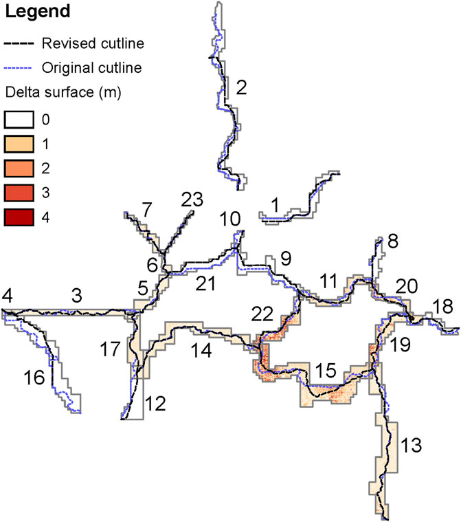
Figure 9 summarizes the differences between the cutlines constructed by conventional (original) process and workflow-based (revised) approach. Figure 9 also illustrates some overlaps with the zero height difference between two surveys. This slight anomaly is due to the way in which the LiDAR surveys were commissioned. Specifically, LiDAR flights were broken into survey extents approximating the boundaries of local councils, such that any LiDAR survey covering a larger area was broken into a set of overlapping smaller surveys.

FIGURE 9

FIGURE 9. Comparison of cutlines with labeled overlap regions and cost surfaces.

The two sets of cutlines are not identical due to differences which can be attributed to the following:

• differences in the algorithms used to calculate the cutline path;

• differences in the placement of cutline endpoints; and

• differences in the weightings used to construct the cost surface.

Difference in cutline path algorithm. In the original SCDEM process, ArcGIS’s “Cost Distance” tool was used on the delta surface to create an accumulative cost surface from the start point. The “Cost Path” tool was then used to find the shortest path through this cost surface to the end point and then converted to vector format using the “Raster to Polyline” tool. While it is likely that these tools operate using some variant of Dijkstra’s algorithm, the exact details of the methods employed in that proprietary software are unknown. As we stated in Section 4, our main aim is to improve reproducibility of the original GA process. However, unknown or hidden information due to use of GIS proprietary and “black box” tools in the original process creates challenges and difficulties in reproducing the cutline construction of the SCDEM. In contrast, our K-span software tool uses the R module “gdistance”, an open-source implementation of Dijkstra’s algorithm and meets the requirements for openness, transparency and automation.

In addition, ArcGIS’s least cost path operates on a “queen’s case” neighborhood of eight adjacent cells (Anselin, 2020). As a result, cutline paths in the original SCDEM process frequently traverse cells diagonally. This in turn increases uncertainty and ambiguity in the cutline construction as it becomes unclear which survey’s raster cell should be chosen for image mosaicking. Hence, this affects the quality and accuracy of the SCDEM. The K-span software tool integrates and uses the R open-source least-cost path algorithm which enables the cutline construction to be restricted to “rook’s case” (i.e., the four cardinal directions) (Anselin, 2020). In particular, this solution allows reduction in spatial uncertainty and avoiding any ambiguity at the boundary of cutlines during image mosaicking.

Difference in the endpoint placement. For three surveys overlap, the placement of cutline endpoints is set at the centroid of the overlapping area, for both original and workflow SCDEM processes. Polygon “centroid” is used to refer to a number of different operations, including the mean center, center of mass, and MBR (minimum bounding rectangle) center (de Smith et al., 2016). However, none of these three measures were found to match the locations of the endpoint placement in the original GA process. This means that these points were most likely placed manually by a human operator. In contrast, our workflow-based approach automated the placement of endpoints by using the center of mass measure in the revised process.

In addition, for cases with two surveys overlap, the original SCDEM process required manual placement of endpoints using human operator judgment in cases where the overlap region terminates as an edge. Our workflow automated the endpoint placements, using a transparent rule that places endpoints always closest to the older survey raster. Hence, this rule effectively maximizes use of larger portion of newer survey by placing the endpoint on the edge of the region overlap between two surveys (see Figure 10).

FIGURE 10

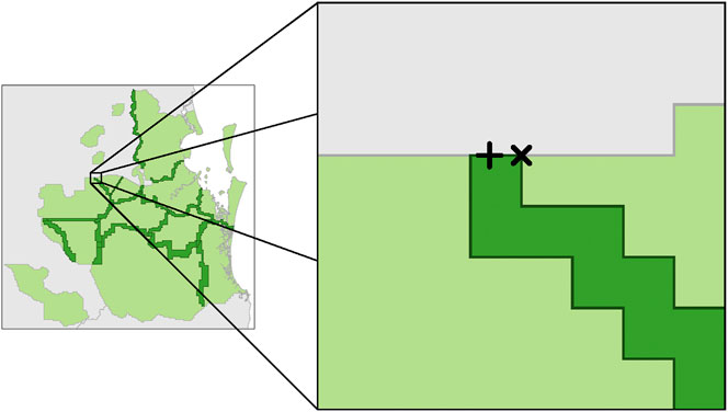
FIGURE 10. Differences between endpoint placement when region overlap (dark green) terminates in an edge. Original process (+) has placed endpoint near the middle whereas revised process (×) is closest to the older survey (light green region on right).

Figure 11 shows the combined Euclidean distance between cutline endpoints. The cutline for overlap 13 was omitted from this and all further comparisons due to corruption in the source data causing the loss of 22 1×1 km tiles since the original SCDEM process was performed. This has resulted in a cutline that travels outside the revised overlap (see Figure 9). While it was found that the distances between endpoints from the original and revised SCDEM processes where three surveys overlap could produce large distances (e.g., cutline 3), differences in endpoint placement where two surveys overlap were found to be much larger (e.g., cutlines 2 and 16). In either case, given that endpoint placement can vary so widely, it is important to have an automated process that will choose the same placement given the same geometry to ensure consistent results.

FIGURE 11

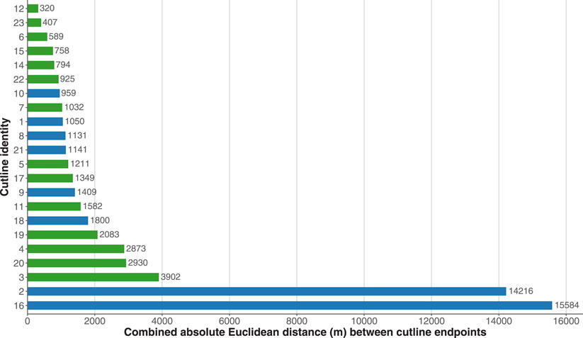
FIGURE 11. Combined Euclidean distance between cutline endpoints. Green indicates cutlines through “same survey” overlap regions; blue cutlines that traverse overlap regions containing different LiDAR surveys.

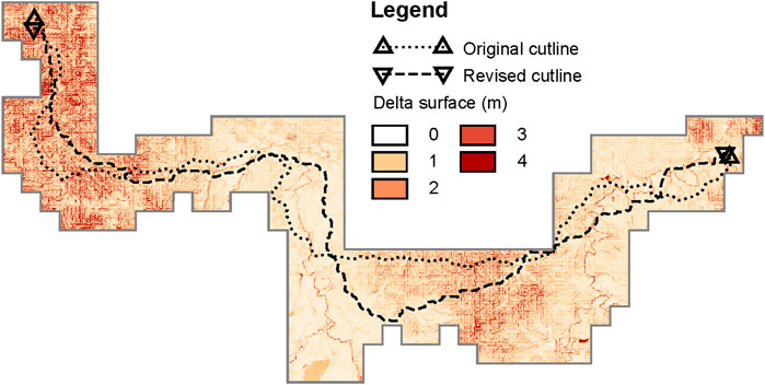
Difference in cost surface. In the original process, the cost surface is simply the absolute difference in heights between the surveys. However, in many cases this can lead to multiple equally low-cost paths between the cutline end points. In turn, this leads the process to arbitrarily select one least-cost path, frequently resulting in highly indirect and sinuous cutlines. This difference is most apparent in overlap 15, with the original cutline moving back and forth across the overlap several times while the revised cutline takes a much more direct path (see Figure 12).

FIGURE 12

FIGURE 12. Comparison of cutlines for overlap 15.

This effect was almost certainly not what was originally intended. Instead our revised workflow-based approach introduces a minute cost related to the length of the path (1 μm per raster cell, which adds a total of 2.9 mm to the cumulative height for the longest revised cutline). This length penalty is small enough to ensure that even the smallest height differences always dominate differences in path length, but that resulting least cost path is reliably also the shortest and most direct of all least cost paths.

5.2.2 Cutline performance

Figure 13 summarizes the quantitative differences in cutlines, in terms of:

(a) the difference in length between pairs of (original and revised) cutlines;

(b) the area enclosed by these pairs (as a proportion of the total area of corresponding survey overlap)

(c) the Hausdorff distance Min et al. (2007) between the two cutlines.

FIGURE 13

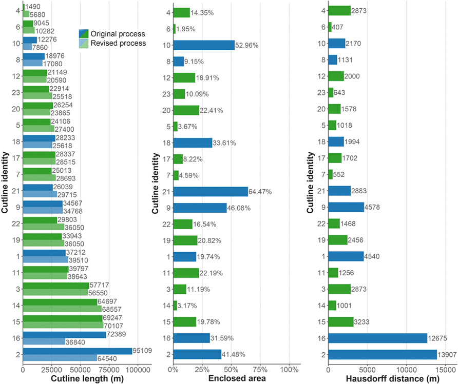
FIGURE 13. Quantitative differences in cutlines showing the length of the original and revised cutlines, area enclosed by the pair of cutlines (as a proportion of the total overlap area), and the Hausdorff distance between the two cutlines. “Same survey” and “Different survey” overlap regions are indicated in green and blue respectively, and are ordered by maximum cutline length.

These observed differences in cutlines arise as a result of the combination of all three factors above: different algorithms, endpoints, and cost surface. However, a few instances of large differences between original and revised cutline lengths were not found statistically significant at the 5% level (p = 0.566) using a Wilcoxon rank sum hypothesis test (Wilcoxon, 1945). Differences do however appear especially marked between those cutlines that relate to overlap regions based on the same original LiDAR survey (i.e., 1, 2, 8, 9, 10, 16, 18, and 21). The Wilcoxon rank sum hypothesis test confirms this apparent difference, with systematically larger differences found to be associated with the “same survey” overlaps when compared with cutlines for overlaps based on different surveys (significant at the 5% level, p = 0.0022 and p = 0.0127 for enclosed proportionate area and Hausdorff distance respectively).

These discrepancies in particular can be attributed to the arbitrariness of selecting one least-cost path from amongst the large number of equally least-cost possibilities in these overlapping regions. Instead, in our workflow, the least-cost path with shortest (Euclidean) distance will consistently be chosen (see Section 5.2.1). This previously unobserved arbitrariness embedded in the original SCDEM procedure becomes more easily observed with “many-eyes” able to scrutinize open K-span workflow.

As a result, the total length of cutlines through “same survey” overlaps is shorter using the revised procedure (255,930 m) than the original procedure (324,802 m). However, a Wilcoxon rank sum hypothesis test shows that this apparent difference between paired original and revised “same survey” cutline lengths is not statistically significant at the 5% level (p = 0.250).

By contrast the same hypothesis test reveals that for the “different survey” overlap regions, the original SCDEM process generates cutlines that are shorter (total length 453,511 m) than the revised process (total length 476,499 m), significant at the 5% level (p = 0.0353).

However, this analysis does not account for differences in the lengths of cutlines due to other factors (such as different endpoint locations). Figure 14 compares the “different survey” cutlines in terms of total cost (in m height) and the unit cost (in m height per m length of cutline). Both the total height difference of cutlines (1,779 m versus 4,856 m height) and the unit cost (0.0037 m height per m distance and 0.0107 m height per m distance) was reduced in our revised SCDEM process. Wilcoxon rank sum hypothesis tests showed that both these differences were significant at the 5% level (p = 0.0494 and p = 0.0067 respectively).

FIGURE 14

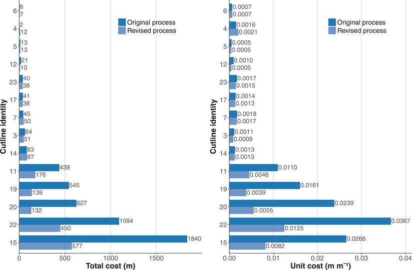
FIGURE 14. Comparison of “Different survey” cutlines in terms of total cost (in m height) and the unit cost (in m height per m length of cutline), ordered by maximum total cost per overlap region.

In summary, taking into account the differences in procedure details, our revised and more transparent workflow-based approach improved the overall performance of the process related to the original goal of reducing total height differences between mosaicked surveys.

6 Discussion and conclusion

In this paper we described the K-span tool, an open-source software solution for reproducible spatial analysis, based on KNIME scientific workflow system. The K-span enables analysts to conduct more open, transparent and automated process of constructing DEM and opportunity to document complex spatial analytics procedures.

Our case study associated to the generation of the SCDEM from LiDAR survey data highlights the benefits accrued from this increased openness and transparency, and improved automation of the process. Overall, the case study has demonstrated how the transition from written documentation and manual process execution to the “executable documentation” provided by K-span software tool and scientific workflow-based approach can aid to more open, transparent, automated and reproducible spatial analytics. In our case study, this included:

• Application, testing and validation of K-span software tool for reproducible spatial analytics;

• Enabling the implementation of the SCDEM process with our workflow-based approach;

• Providing a graphical description of the processes involved in generating the DEM;

• Automating human judgment in selecting cutline endpoints;

• Exposing differences in the implementation of basic spatial operations, such as in shortest path and centroid calculation between Esri’s ArcGIS and our K-span software tools;

• Enabling the replacement of closed proprietary routines with open-source alternatives; and

• Revealing unintended discrepancies in the computation of cost surfaces, affording greater scrutiny of analytics processes by “many eyes.”

Together, this improved ability to scrutinize spatial analytics can contribute to increasing the assurance and confidence of foundational spatial data sets, such as the Australian national DEM. Using scientific workflow-based tools such as our K-span for reproducible spatial analytics makes explicit the provenance of data, not simply as accuracy/precision metadata nor through written documentation, but by linking the software and parameters used to the raw data sets via the automated and unambiguous sequence of spatial data operations.

The scope of this work excluded analysis for computational efficiency of the K-span software tool. In particular, demonstrating the difference in computational efficiency between the original GA process and our workflow-based approach was not part of this study. Hence, future research may include testing on this property of the K-span software tool. Also, future work will focus on increasing the scalability of the K-span software tool. This will involve replacing the current string-based data model for storing geometry with a more efficient object-based model as well as improving the parallelization of the system. Presently, nodes use naive parallization, where each row of a table is sent individually to the job queue. Given that sending jobs incurs a cost, fast jobs can spend more of their time managing the job queue than processing the data. By implementing a more intelligent parallelization scheme, rows can be dynamically grouped into jobs to achieve the optimum balance between job size and queue length.

A longer term goal is the development of a new language for spatial analysis, in a similar vein to Vahedi et al. (2016), where users focus on asking questions about spatial data instead of performing operations. Given the current nodes are modeled after the spatial operations found in PostGIS, this will involve a complete restructuring of operations to fit the new paradigm.

7 Software availability

The K-span software tool is available under an open-source license and the source code and latest releases are available in the following GitHub repository and an overview of our reference case study and documentation related to installation and use of the platform can be found at the following links:

• https://github.com/OpenSpatialAnalytics/ga-osa

• https://sites.rmit.edu.au/openspatialanalytics/

Data availability statement

The datasets presented in this study can be found in online repositories. The names of the repository/repositories and accession number(s) can be found below: https://github.com/OpenSpatialAnalytics/ga-osa https://sites.rmit.edu.au/openspatialanalytics/.

Author contributions

AF lead the paper and contributed to all sections in the manuscript including developing new geospatially enabled workflows nodes and processing spatial data and executing workflows. AB lead the paper and contributed to all sections in the manuscript including developing new geospatially enabled workflows nodes and processing spatial data and executing workflows. CB contributed to Sections 2, 3, 4, 5 of the manuscript. MD contributed to Sections 1, 2, 3, 4, 6 of the manuscript. HA contributed to Sections 4, 5 including processing original data set provided by Geoscience Australia. NR contributed to Sections 1, 2, 6.

Conflict of interest

The authors declare that the research was conducted in the absence of any commercial or financial relationships that could be construed as a potential conflict of interest.

Publisher’s note

All claims expressed in this article are solely those of the authors and do not necessarily represent those of their affiliated organizations, or those of the publisher, the editors and the reviewers. Any product that may be evaluated in this article, or claim that may be made by its manufacturer, is not guaranteed or endorsed by the publisher.

Footnotes

¹http://gdal.org.

²http://qgis.org.

³http://postgis.net.

⁴https://www.knime.com/.

⁵Geoscience Australia, http://www.ga.gov.au.

⁶https://kepler-project.org/.

⁷https://oceanservice.noaa.gov/facts/lidar.html.

⁸https://www.vistrails.org//index.php/Main_Page.

⁹https://incubator.apache.org/projects/taverna.html.

¹⁰https://www.osgeo.org/projects/jts/.

¹¹https://www.ogc.org/standards/geoapi.

¹²https://geojson.org/.

¹³https://www.json.org/json-en.html.

¹⁴https://www.knime.com/developer/documentation/node-dialog.

¹⁵https://sites.rmit.edu.au/openspatialanalytics/osa-node-rep/shapefile-reader/.

¹⁶https://doc.arcgis.com/en/arcgis-online/reference/shapefiles.htm.

¹⁷https://sites.rmit.edu.au/openspatialanalytics/osa-node-rep/shapefile-writer/.

¹⁸https://sites.rmit.edu.au/openspatialanalytics/osa-node-rep/buffer/.

¹⁹https://www.ogc.org/standards/wfs.

²⁰https://pro.arcgis.com/en/pro-app/latest/help/analysis/geoprocessing/modelbuilder/what-is-modelbuilder-.htm.

²¹https://www.safe.com/solutions/ (FME).

²²https://www.anzlic.gov.au/resources/foundation-spatial-data-framework/fsdf-themes-datasets/elevation-and-depth.

²³https://gisgeography.com/raster-resampling/.

²⁴https://www.l3harrisgeospatial.com/docs/mosaicseamless.html.

²⁵https://cran.r-project.org/web/packages/gdistance/index.html.

References

Anselin, L. (2020). Contiguity-based spatial weights. Available on: https://geodacenter.github.io/workbook/4a_contig_weights/lab4a.html.

Google Scholar

Bakos, G. (2013). KNIME essentials. Birmingham, United Kingdom: Packt Publishing. Available on: https://books.google.com.au/books?id=jXNZAQAAQBAJ.

Google Scholar

Barker, A., and Van Hemert, J. (2007). “Scientific workflow: A survey and research directions,” in International Conference on Parallel Processing and Applied Mathematics (Springer), 746–753.

Google Scholar

Barseghian, D., Altintas, I., Jones, M. B., Crawl, D., Potter, N., Gallagher, J., et al. (2010). Workflows and extensions to the kepler scientific workflow system to support environmental sensor data access and analysis. Ecol. Inf. 5 (1), 42–50. doi:10.1016/j.ecoinf.2009.08.008

CrossRef Full Text | Google Scholar

Berthold, M. R., Cebron, N., Dill, F., Gabriel, T. R., Kötter, T., Meinl, T., et al. (2009). KNIME-The konstanz information miner: Version 2.0 and beyond. AcM SIGKDD Explor. Newsl. 11 (1), 26–31. doi:10.1145/1656274.1656280

CrossRef Full Text | Google Scholar

Brown, D. A., Brady, P. R., Dietz, A., Cao, J., Johnson, B., and McNabb, J. (2007). “A case study on the use of workflow technologies for scientific analysis: Gravitational wave data analysis,” in Workflows for e-Science (Springer), 39–59.

Google Scholar

Butler, H., Daly, M., Doyle, A., Gillies, S., Hagen, S., and Schaub, T. (2016). The geojson format. Tech. rep. Reston, VA: Internet Engineering Task Force.

CrossRef Full Text | Google Scholar

Cagnacci, F., and Urbano, F. (2008). Managing wildlife: A spatial information system for gps collars data. Environ. Model. Softw. 23 (7), 957–959. doi:10.1016/j.envsoft.2008.01.003

CrossRef Full Text | Google Scholar

Callaghan, S., Deelman, E., Gunter, D., Juve, G., Maechling, P., Brooks, C., et al. (2010). Scaling up workflow-based applications. J. Comput. Syst. Sci. 76 (6), 428–446. doi:10.1016/j.jcss.2009.11.005

CrossRef Full Text | Google Scholar

Cerutti, V., Bellman, C., Both, A., Duckham, M., Jenny, B., Lemmens, R. L. G., et al. (2021). Improving the reproducibility of geospatial scientific workflows: The use of geosocial media in facilitating disaster response. J. Spatial Sci. 66 (3), 383–400. doi:10.1080/14498596.2019.1654944

CrossRef Full Text | Google Scholar

Cohen-Boulakia, S., Belhajjame, K., Collin, O., Chopard, J., Froidevaux, C., Gaignard, A., et al. (2017). Scientific workflows for computational reproducibility in the life sciences: Status, challenges and opportunities. Future Gener. Comput. Syst. 75, 284–298. doi:10.1016/j.future.2017.01.012

CrossRef Full Text | Google Scholar

Crawl, D., and Altintas, I. (2008). “A provenance-based fault tolerance mechanism for scientific workflows,” in Provenance and annotation of data and processes (Berlin, Heidelberg: Springer), 152–159. doi:10.1007/978-3-540-89965-5_17

CrossRef Full Text | Google Scholar

de Smith, M., Longley, P., and Goodchild, M. (2016). Geospatial analysis: A comprehensive guide. UK: The Winchelsea Press.

Google Scholar

Dietz, C., and Berthold, M. R. (2016). KNIME for open-source bioimage analysis: A tutorial. Springer International Publishing, 179–197. doi:10.1007/978-3-319-28549-8_7

CrossRef Full Text | Google Scholar

ESRI (2021). ST_Transform. Available on: https://desktop.arcgis.com/en/arcmap/latest/manage-data/using-sql-with-gdbs/st-transform.htm.

Google Scholar

Freire, J., Koop, D., Chirigati, F., and Silva, C. (2018). Reproducibility using VisTrails, 2, 33–56. doi:10.1201/9781315373461-2

CrossRef Full Text | Google Scholar

Geoscience Australia (2015). Digital elevation model (DEM) of Australia derived from LiDAR 5 metre grid. doi:10.4225/25/5653D877D3E08

CrossRef Full Text | Google Scholar

Horsburgh, J. S., Reeder, S. L., Jones, A. S., and Meline, J. (2015). Open source software for visualization and quality control of continuous hydrologic and water quality sensor data. Environ. Model. Softw. 70, 32–44. doi:10.1016/j.envsoft.2015.04.002

CrossRef Full Text | Google Scholar

Hull, D., Wolstencroft, K., Stevens, R., Goble, C., Pocock, M. R., Li, P., et al. (2006). Taverna: A tool for building and running workflows of services. Nucleic acids Res. 34 (2), W729–W732. doi:10.1093/nar/gkl320

PubMed Abstract | CrossRef Full Text | Google Scholar

Jaeger, E., Altintas, I., Zhang, J., Ludäscher, B., Pennington, D., and Michener, W. (2005). “A scientific workflow approach to distributed geospatial data processing using web services,” in Proceedings of the 17th International Conference on Scientific and Statistical Database Management. SSDBM’2005, Berkeley, USA (Berkeley, CA: Lawrence Berkeley Laboratory), 87–90.

Google Scholar

Kitzes, J., Turek, D., and Deniz, F. (2018). The practice of reproducible research: Case studies and lessons from the data-intensive sciences. 1st Edition. University of California Press.

Google Scholar

Leonard, L., and Duffy, C. (2016). Visualization workflows for level-12 HUC scales: Towards an expert system for watershed analysis in a distributed computing environment. Environ. Model. Softw. 78, 163–178. doi:10.1016/j.envsoft.2016.01.001

CrossRef Full Text | Google Scholar

Liew, C. S., Atkinson, M. P., Galea, M., Ang, T. F., Martin, P., and Hemert, J. I. V. (2016). Scientific workflows: Moving across paradigms. ACM Comput. Surv. 49 (4), 1–39. doi:10.1145/3012429

CrossRef Full Text | Google Scholar

Ludäscher, B., Altintas, I., Berkley, C., Higgins, D., Jaeger, E., Jones, M., et al. (2006). Scientific workflow management and the Kepler system. Concurrency Comput. Pract. Exp. 18 (10), 1039–1065. doi:10.1002/cpe.994

CrossRef Full Text | Google Scholar

Ludäscher, B., Weske, M., McPhillips, T., and Bowers, S. (2009). “Scientific workflows: Business as usual?,” in Business process management. Editors U. Dayal, J. Eder, J. Koehler, and H. A. Reijers (Berlin, Heidelberg: Springer Berlin Heidelberg), 31–47.

Google Scholar

McFerren, G., Van Zyl, T., and Vahed, A. (2012). Foss geospatial libraries in scientific workflow environments: Experiences and directions. Appl. Geomatics 4 (2), 85–93. doi:10.1007/s12518-011-0062-0

CrossRef Full Text | Google Scholar

Min, D., Zhilin, L., and Xiaoyong, C. (2007). Extended hausdorff distance for spatial objects in gis. Int. J. Geogr. Inf. Sci. 21 (4), 459–475. doi:10.1080/13658810601073315

CrossRef Full Text | Google Scholar

Morisette, J. T., Jarnevich, C. S., Holcombe, T. R., Talbert, C. B., Ignizio, D., Talbert, M. K., et al. (2013). Vistrails sahm: Visualization and workflow management for species habitat modeling. Ecography 36 (2), 129–135. doi:10.1111/j.1600-0587.2012.07815.x

CrossRef Full Text | Google Scholar

Neteler, M., Bowman, M. H., Landa, M., and Metz, M. (2012). Grass gis: A multi-purpose open source gis. Environ. Model. Softw. 31, 124–130. doi:10.1016/j.envsoft.2011.11.014

CrossRef Full Text | Google Scholar

Obe, R. O., and Hsu, L. S. (2015). PostGIS in action. New York, NY: Manning Publications Co.

Google Scholar

Peng, R. D. (2011). Reproducible research in computational science. Science 334 (6060), 1226–1227. doi:10.1126/science.1213847

PubMed Abstract | CrossRef Full Text | Google Scholar

Radosevic, N., Duckham, M., Liu, G.-J., and Sun, Q. (2020). Solar radiation modeling with knime and solar analyst: Increasing environmental model reproducibility using scientific workflows. Environ. Model. Softw. 132, 104780. doi:10.1016/j.envsoft.2020.104780

CrossRef Full Text | Google Scholar

Riaño-Briceño, G., Barreiro-Gomez, J., Ramirez-Jaime, A., Quijano, N., and Ocampo-Martinez, C. (2016). Matswmm–an open-source toolbox for designing real-time control of urban drainage systems. Environ. Model. Softw. 83, 143–154. doi:10.1016/j.envsoft.2016.05.009

CrossRef Full Text | Google Scholar

Sangireddy, H., Stark, C. P., Kladzyk, A., and Passalacqua, P. (2016). Geonet: An open source software for the automatic and objective extraction of channel heads, channel network, and channel morphology from high resolution topography data. Environ. Model. Softw. 83, 58–73. doi:10.1016/j.envsoft.2016.04.026

CrossRef Full Text | Google Scholar

Scheider, S., and Ballatore, A. (2017). Semantic typing of linked geoprocessing workflows. Int. J. Digital Earth 0 (0), 113–138. doi:10.1080/17538947.2017.1305457

CrossRef Full Text | Google Scholar

Shekhar, S., and Xiong, H. (2008). “Java topology suite (JTS),” in Encyclopedia of GIS (Springer), 601.

CrossRef Full Text | Google Scholar

Sun, S., Chen, J., Li, W., Altintas, I., Lin, A., Peltier, S., et al. (2011). Community cyberinfrastructure for advanced microbial ecology research and analysis: The CAMERA resource. Nucleic Acids Res. 39 (1), D546–D551. doi:10.1093/nar/gkq1102

PubMed Abstract | CrossRef Full Text | Google Scholar

Thorp, K., and Bronson, K. (2013). A model-independent open-source geospatial tool for managing point-based environmental model simulations at multiple spatial locations. Environ. Model. Softw. 50, 25–36. doi:10.1016/j.envsoft.2013.09.002

CrossRef Full Text | Google Scholar

Turuncoglu, U. U., Dalfes, N., Murphy, S., and DeLuca, C. (2013). Toward self-describing and workflow integrated Earth system models: A coupled atmosphere-ocean modeling system application. Environ. Model. Softw. 39, 247–262. doi:10.1016/j.envsoft.2012.02.013

CrossRef Full Text | Google Scholar

Vahedi, B., Kuhn, W., and Ballatore, A. (2016). “Question-based spatial computing – a case study,” in Geospatial data in a changing world. Lecture notes in geoinformation and cartography (Cham: Springer), 37–50. doi:10.1007/978-3-319-33783-8_3

CrossRef Full Text | Google Scholar

van Etten, J. (2017). R package gdistance: Distances and routes on geographical grids. J. Stat. Softw. 76 (13), 21. doi:10.18637/jss.v076.i13

CrossRef Full Text | Google Scholar

Wang, J., Crawl, D., and Altintas, I. (2012). A framework for distributed data-parallel execution in the kepler scientific workflow system. Procedia Comput. Sci. 9, 1620–1629. doi:10.1016/j.procs.2012.04.178

CrossRef Full Text | Google Scholar

Warmerdam, F. (2008). “The geospatial data abstraction library,” in Open source approaches in spatial data handling (Springer), 87–104.

Google Scholar

Warr, W. A. (2012). Scientific workflow systems: Pipeline pilot and knime. J. computer-aided Mol. Des. 26 (7), 801–804. doi:10.1007/s10822-012-9577-7

PubMed Abstract | CrossRef Full Text | Google Scholar

Wilcoxon, F. (1945). Individual comparisons by ranking methods. Biom. Bull. 1 (6), 80–83. doi:10.2307/3001968

CrossRef Full Text | Google Scholar

Wilkinson, M. D., Dumontier, M., Aalbersberg, I. J., Appleton, G., Axton, M., Baak, A., et al. (2016). The FAIR guiding principles for scientific data management and stewardship. Sci. Data 3 (1), 160018–160019. doi:10.1038/sdata.2016.18

PubMed Abstract | CrossRef Full Text | Google Scholar

Yin, D., Liu, Y., Hu, H., Terstriep, J., Hong, X., Padmanabhan, A., et al. (2018). CyberGIS-Jupyter for reproducible and scalable geospatial analytics. Concurrency Comput. Pract. Exp. 31 (11), 1–16. doi:10.1002/cpe.5040

CrossRef Full Text | Google Scholar

Yue, P., Zhang, M., and Tan, Z. (2015). A geoprocessing workflow system for environmental monitoring and integrated modelling. Environ. Model. Softw. 69, 128–140. doi:10.1016/j.envsoft.2015.03.017

CrossRef Full Text | Google Scholar

Zhang, J., Pennington, D. D., and Michener, W. K. (2006). “Automatic transformation from geospatial conceptual workflow to executable workflow using grass gis command line modules in kepler,” in Computational science – ICCS 2006. Editors V. N. Alexandrov, G. D. van Albada, P. M. A. Sloot, and J. Dongarra (Berlin, Heidelberg: Springer Berlin Heidelberg), 912–919.

CrossRef Full Text | Google Scholar

Zyl, T. L. v., Vahed, A., McFerren, G., and Hohls, D. (2012). Earth observation scientific workflows in a distributed computing environment. Trans. GIS 16 (2), 233–248. doi:10.1111/j.1467-9671.2012.01317.x

CrossRef Full Text | Google Scholar