One-degree resolution mascon solution over Antarctic derived from GRACE Level-2 data

The mass loss of the Antarctic Ice Sheet (AIS) is an important contributor to global sea-level rise in response to the warming ocean and atmospheric temperatures as well as the changes in current systems and precipitation patterns. In this study, a regional mascon method is developed to squeeze more mass change signals, in which the pseudo-observations of the geopotential are generated from the unfiltered GRACE Level-2 data whereas the regularization matrix is constructed with the prior information derived from filtered GRACE Level-2 data. A series of mascon solutions with $\mathbf{1}°\times \mathbf{1}°$ equal-area resolution over AIS is derived from the updated Tongji-Grace2018 model spanning April 2002 to December 2016. Compared to the filtering results from P4M6 decorrelation and 100 km Gaussian filtering, our mascon solutions can effectively suppress the strips, improve the spatial resolution over AIS, and get a stronger signal with an improvement of 116.86% in the Antarctic Peninsula Ice Sheet (APIS), and more coincide with the features of glaciers and ice streams, such as the most striking ice mass loss in Totten, Getz, Thwaites and Pine Island, and the ice mass gain in Kamb Ice Stream. During the period from 2002 to 2016, the mass change rates from our mascon solution are −103.6 ± 5.6 Gt/yr, 63.0 ± 4.3 Gt/yr, −143.3 ± 4.9 Gt/yr and −23.29 ± 1.2 Gt/yr in AIS, East AIS, West AIS, and APIS, respectively. The mass change signals at the basin scale are with even more distinguishing features, with the highest mass gain rates of 18.03 ± 1.88 Gt/yr and 14.55 ± 0.60 Gt/yr at Basin 7 and Basin 18, and the highest mass loss rates of −58.57 ± 2.48 Gt/yr and −44.12 ± 2.27 Gt/yr at Basin 21 and Basin 22. Relative to the cumulated surface mass balance from the regional atmospheric climate model, the correlation coefficients of our mascon solutions are 0.91, 0.94, and 0.96 in East AIS, West AIS, and APIS.

1 Introduction

The contribution to global sea-level rise from the melting of polar ice sheets has been a focus of intensive study over the past several decades (Harig and Simons, 2012; Iz et al., 2021). As the largest ice sheet over the globe, the Antarctic Ice Sheet (AIS) is one of the major contributors to global mean sea level rise (Vaughan et al., 2013; Pattyn et al., 2018; Rignot et al., 2019). Therefore, the accurate estimate of mass changes over AIS is of utmost importance (Shepherd et al., 2018). Since the advent of satellite observations, three types of techniques have been used to estimate the mass balance over AIS: 1) Satellite altimetry method at intermediate resolution (1–10 km) by using the direct measurements of elevation changes combined with climatological/glaciological models for firn (snow) density and compaction (Shepherd et al., 2019); 2) input-output method (IOM) at a high resolution (100 m–1 km) by measuring the ice flow velocities with synthetic aperture radar data over outlet glaciers combined with glacier thickness data to derive the ice discharge and surface mass balance (SMB) (van Wessem et al., 2018; Rignot et al., 2019); 3) satellite gravimetry and airborne gravimetry by measuring the gravity change due to ice mass variation, such as the satellite mission of gravity recovery and climate experiment (GRACE) (Velicogna and Wahr, 2006). Besides the GRACE mission, the other two techniques can hardly directly provide the AIS mass estimation with the monthly resolution, single satellite altimetry is restricted by temporal sampling issues and converting elevation change into mass change which requires assumptions on density due to firn density not known very well (Khan et al., 2015), and the penetration depth of radar altimetry may change during seasons of freezing-thaw (Nilsson et al., 2015). The IOM is limited by the annual temporal resolution of ice discharge (Rignot et al., 2019).

GRACE provides the direct measurement of ice mass change with a temporal resolution of 1 month at an error level of 2 cm in terms of equivalent water height (EWH) (Wahr et al., 2006; Tapley et al., 2019), which is less influenced by the temporal sampling issues and unknown surface properties compared to the single satellite altimetry mission. By using the GRACE gravity field solutions, many estimates related to the mass loss rates over AIS have been achieved (Table 1), though these results are very different from 67 ± 44 Gt/yr (Velicogna et al., 2014) to 165 ± 72 Gt/yr (Jacob et al., 2012), due to using different GRACE solutions, different Glacial Isostatic Adjustment (GIA) models and methodologies, as well as in different periods. Previous studies mainly focus on the estimation at large scale, i.g., the whole AIS, west AIS, east AIS, and APIS, since the estimation at the basin scale is limited by the GRACE spatial resolution. Moreover, the AIS mass changes before and after the epoch between 2007–2008 are quite different (Loomis et al., 2019a; Loomis et al., 2020), which are worthy to be further investigated.

TABLE 1

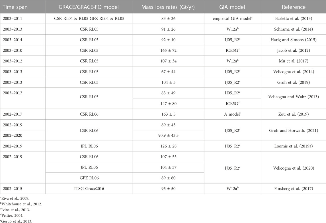
TABLE 1. Mass loss rates over AIS with GIA corrections.

The GRACE gravity field solutions are expressed in terms of spherical harmonic coefficients (SHCs) or mascon solutions. Since significant north-south striping errors exist in the map of estimated mass change directly from GRACE SHCs solutions, several post-processing techniques, such as Gaussian filters (Jekeli, 1981; Wahr et al., 1998), decorrelation filters (Swenson and Wahr, 2006), and DDK filters (Kusche et al., 2009), have been developed to mitigate these errors. However, these filters all cause the attenuation of real geophysical signals (Tapley et al., 2019) and leakage errors that reach 20 Gt/yr in AIS (Chen et al., 2015; Mu et al., 2017). To mitigate leakage error and increase the spatial resolution, Chen et al. (2021) developed the global regularized SHC solutions up to degree and order (d/o) 180 that is comparable with the three global mascon solutions, e.g., CSR (Center for Space Research, the University of Texas) mascon (Save et al., 2016), JPL (Jet Propulsive Laboratory) mascon (Watkins et al., 2015) and GSFC (Goddard Space Flight Center) mascon (Loomis et al., 2019b) solutions. JPL and GSFC mascon solutions are both developed from the GRACE Level-1B observations while CSR mascon solution is generated from the SHCs up to degree and order 120. The regularization matrix is constructed differently, from the GRACE information (CSR), the prior geophysical signals (JPL), and the spatial/temporal correlated exponential function (GSFC). However, operating on the Level-1B observations is very complex with a huge computation burden, and the implementation and further improvement of them are almost impossible for others (Baur and Sneeuw, 2011; Ran, 2017). Besides, different global mascon solutions show obvious discrepancies at the regional scale for hydrology (Scanlon et al., 2016). For example, the JPL mascon solution overestimates the decreasing and increasing rates of the terrestrial water storage anomalies (TWSA) over the Tibet Plateau relative to other GRACE solutions (Jing et al., 2019). Moreover, when focusing on the signals at the region less than $3°\times 3°$, global mascon solutions should be used with caution (Zhang et al., 2019). Therefore, the SHCs are still used as the standard solutions for GRACE data while needing further processing to reduce noise in higher degree SHCs and restore regional signals due to the cut-off of SHCs. The regional mascon method utilizes the SHCs to generate the observations, also called pseudo-observations, the mascons to be solved are set in the place interested with the expected resolution, and only regional prior information is needed to construct the regularization matrix, therefore it is much easier to be implemented (Ran, 2017). The pseudo-observations can be either the geoid heights (Sasgen et al., 2010), filtered mass changes at the ground (Schrama and Wouters, 2011; Yi and Sun, 2014) or the radial gravity disturbances at mean satellite altitude (Forsberg and Reeh, 2007; Sørensen and Forsberg, 2010; Baur and Sneeuw, 2011). Among these pseudo-observations, the radial gravity disturbances at GRACE satellite altitude are more natural as the synthesized data better resemble original observations at satellite altitude. However, the observation information in the other two directions is usually abandoned except for Su et al. (2019) who considered the pseudo-observations of three directions in their mascon solutions. Moreover, previous studies on the regional mascon methods did not pay enough attention to the construction of the regularization matrix and used an identity matrix as a regularization matrix to stabilize the mascon solutions (Forsberg and Reeh, 2007; Sørensen and Forsberg, 2010; Baur and Sneeuw, 2011; Barletta et al., 2013; Yi and Sun, 2014). However, the regularization matrix plays an important role in leakage error correction and should reflect the power spectrum of the parameters. Using an identity matrix means all parameters with the same power spectrum and the signal leakage remains between adjacent basins (Barletta et al., 2013). Therefore, we introduce the regularization matrix with prior information from filtered GRACE SHCs into the mascon modeling method to reduce signal leakage and improve the spatial resolution of the mascon solutions.

Considering gravity disturbance contains full gravity information, in this paper, we propose a gravitational potential-based regional mascon method where the gravity disturbance at satellite altitude is used as the pseudo-observations to construct the observation equation. The proposed mascon method is used to derive the regional mascon solutions over AIS from April 2002 to December 2016 with a regularization matrix constructed with the prior information from filtered SHCs. The generated mascon solutions are first compared with the filtered counterparts to preliminary show the improvement in signal recovery and the sensitivity of mascon solutions to the prior information. Then, the spatiotemporal mass change signals of our mascon solutions over AIS are analyzed in different periods by compared with those of CSR, GSFC, and JPL mascon solutions. Subsequently, using the detrend mass change of the monthly time series of cumulative surface mass balance (SMB) from the regional atmospheric climate model (RACMO), the interannual mass change variations over AIS and its subregions are also analyzed. The rest of the paper is organized as follows. The used data and proposed mascon method are described in Section 2, 3 respectively. In Section 4, the mascon solutions are generated, and then the mass change rates and interannual signals over AIS are analyzed. Finally, conclusion are drawn in Section 5.

2 Data

2.1 GRACE data

The Tongji-Grace2018 model up to degree and order 90 (Chen et al., 2019) from April 2002 to December 2016 is used in our mascon solutions. The Earth’s geo-center corrections are applied with the degree-1 coefficients from Technical Note-13 (Swenson et al., 2008; Sun et al., 2016). All C₂₀ coefficients of the Tongji-Grace2018 model are replaced by those from Technical Note-14 as recommended by Loomis et al. (2020) and the C₃₀ terms after August 2016 are also replaced by those from Technical Note-14 (Loomis et al., 2019a; Loomis et al., 2020). The regional IJ05_R2 model is applied to correct the long-term GIA signals (Ivins et al., 2013).

Three global mascon solutions from the CSR (Save et al., 2016), GSFC (Loomis et al., 2019b) and JPL (Watkins et al., 2015) are also used to compare the results of our mascon solutions. The CSR mascon solutions can be downloaded from the website of http://www2.csr.utexas.edu/grace/RL06_mascons.html, the GSFC mascon solutions from the link https://earth.gsfc.nasa.gov/geo/data/grace-mascons and JPL mascon solutions from https://grace.jpl.nasa.gov/data/get-data/jpl_global_mascons. It is worthwhile to mention that the three GRACE mascon solutions all use the global ICE-6G model (Peltier, et al., 2018) to remove the GIA signals. To directly compare the results with the previous studies, we added back the GIA signals with the ICE-6G model and then deduct the GIA signals with the IJ05_R2 model according to the recommendation of Ivins et al. (2013).

2.2 RACMO data

The regional atmospheric climate model (RACMO) is developed by the Institute for Marine and Atmospheric Research Utrecht at Utrecht University. RACMO generates the SMB at 27-km resolution by using the physics package of the Integrated Forecast System of the European Centre for Medium-Range Weather Forecasts along with the High-Resolution Limited Area Model (Undén et al., 2002; van Wessem et al., 2014; Rignot et al., 2019). The new release version RACMO2.3p2 spanning from 1979 to 2016, which is updated from RACMO2.3p1, including improved topography, precipitation, and snow properties (van Wessem et al., 2018), is used to compute the interannual variation of surface mass balance over AIS. The time series of cumulative SMB anomalies relative to the average of 1979–2008 (Velicogna et al., 2014; Rignot et al., 2019) are then deducted with the average of the study period, the same as that in processing the GRACE time series. Focusing on the annual and interannual variability over AIS, the ice discharge and linear trend from cumulative SMB should be excluded. Therefore, we finally detrend the GRACE series and cumulative SMB series and apply a 7-month smooth to them.

3 Mascon modeling and its regularized solution

3.1 Gravitational potential-based mascon modeling

Taking the Earth’s elastic deformation into account, the disturbing gravitational potential ${\delta T}_i$ at GRACE satellite attitude can be computed with the unfiltered SHCs as follows,

${\delta T}_i=T\left({\lambda }_i,{\phi }_i,\rho \right)=\frac{GM}{\rho }{\displaystyle \sum }_{l=1}^{l_{\mathit{max}}}{\left(\frac{a}{\rho }\right)}^l\frac{1}{\left(1+k_l^{\prime }\right)}{\displaystyle \sum }_{m=0}^l{P}_{lm}{\left(\sin {\phi }_i)(∆C\right.}_{lm}\cos m{\lambda }_i+{∆S}_{lm}\sin m{\lambda }_i)(1)$

where, $\left({\lambda }_i,{\phi }_i,\rho \right)$ are longitude, latitude, and radial distance of a space point, a is the radial distance of the points at the ellipsoidal surface and it is the function of the latitude, i.e., $a=R\left(1-f\right)/\sqrt{1-{\mathit{sin}}^2\theta }$, $R$ is the radius of the spherical Earth, $f$ is the ellipsoid flattening (WGS84 value: $f=1/298.257223563$) and $\theta$ is the colatitude (Li et al., 2017; Ditmar 2018). $\rho =a+500\mathrm{k}\mathrm{m}$, $GM$ indicates the product of gravitational constant $G$ and the mass of the Earth $M$, $P_{lm}$ denotes the fully normalized associated Legendre functions of degree $l$ and order $m$, $k_l^{\prime }$ is the load Love number of degree $l$; ${∆C}_{lm}$ and ${∆S}_{lm}$ are the unfiltered SHCs after the mean for the study period is removed, $l_{\mathit{max}}$ is the maximum degree.

Figure 1 shows the geometry of the space location $S\left({\lambda }_i,{\phi }_i,\rho \right)$ at the satellite attitude and ground point $P\left({\lambda }_j,{\phi }_j,a\right)$, where a point disturbing mass is located; $d_{i,j}$ and ${\psi }_{i,j}$ are the Euclidean distance and spherical distance between $S\left({\lambda }_i,{\phi }_i,\rho \right)$ and $P\left({\lambda }_j,{\phi }_j,a\right)$.

FIGURE 1

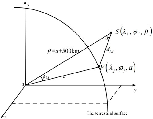
FIGURE 1. Geometry of mascon modeling.

Supposing the disturbing potential ${\delta T}_i$ at point $i$ is caused by the t points of mass anomalies in the study area, according to Newton’s law of gravitation we have the following expression,

${\delta T}_i=G{\displaystyle \sum }_{j=1}^t\frac{\delta m_j}{{\left(a^2+{\rho }^2-2a\rho \cos {\psi }_{i,j}\right)}^{1/2}}(2)$

where $\delta m_j$ is the point mass anomaly at the location $j$. Since the disturbing potential ${\delta T}_i$ is derived from the SHCs with Eq. 1, it is called pseudo-observation, and the point mass unknown $\delta m_j$ can be solved from Eq. 2 with the pseudo-observations over the study area. If there are $n$ $\left(n>t\right)$ number of pseudo-observations, we reformulate Eq. 2 in the matrix form as follows,

$\mathit{y}=\mathit{A}\mathit{x}+\mathit{e}(3)$

where $\mathit{y}={\left(\begin{array}{ccc}{\delta T}_1& \cdots & {\delta T}_n\end{array}\right)}^T$ denotes the $n$-vector of observations, $\mathit{A}$ is an $n\times t$ design matrix (its $ij$ th element $\mathit{A}\left(i,j\right)=G\frac{1}{{\left(a^2+{\rho }^2-\mathit{2}ar\mathit{cos}{\psi }_{i,j}\right)}^{1/2}}$ ), $\mathit{x}$ is a $t$-vector of mass anomalies to be estimated, $\mathit{e}\sim \left(0,{\mathrm{\sigma }}_0^2{\mathit{P}}^{-\mathbf{1}}\right)$ represents the random error vector, ${\mathrm{\sigma }}_0^2$ and $\mathit{P}$ are the variance of unit weight and the weight matrix. The weight matrix $\mathit{P}$ can be directly derived from Eq. 1 via the law of error propagation as $\mathit{P}={\left(\mathit{B}\mathit{D}{\mathit{B}}^{\mathit{T}}\right)}^{-1}$, where $\mathit{D}$ is the full covariance matrix of the SHCs and it can be obtained from the inverse of the normal equation when solving the SHCs. $\mathit{B}$ is the coefficient matrix when the right hand of Eq. 1 is written in a matrix-vector form. The $i$ th row elements of $\mathit{B}$ are expressed as (Chen et al., 2020),

$\left\{\begin{array}{c}\mathit{B}\left(i,j_{{∆C}_{lm}}\right)=\frac{\mathrm{G}\mathrm{M}}{\rho }{\left(\frac{a}{\rho }\right)}^l\frac{1}{1+k_l^{\prime }}{P}_{lm}{\left(\sin {\phi }_i\right)\cos m\lambda }_i\\ \mathit{B}\left(i,j_{{∆S}_{lm}}\right)=\frac{\mathrm{G}\mathrm{M}}{\rho }{\left(\frac{a}{\rho }\right)}^l\frac{1}{1+k_l^{\prime }}{P}_{lm}{\left(\sin {\phi }_i\right)\mathrm{s}\mathrm{i}\mathrm{n}m\lambda }_i\end{array}\right.(4)$

where, $j_{{∆C}_{lm}}$ and $j_{{∆S}_{lm}}$ are the column numbers corresponding to ${∆C}_{lm}$ and ${∆S}_{lm}$, respectively.

3.2 Regularized solution to the ill-conditioned mascon modeling

Since Eq. 3 is ill-conditioned, it is usually solved with Tikhonov regularization and the solution is derived by minimizing the following cost function (Tikhonov, 1963),

$\mathrm{\Phi }\left(\mathit{x}\right)={\left(\mathit{y}-\mathit{A}\mathit{x}\right)}^{\mathrm{T}}\mathit{P}\left(\mathit{y}-\mathit{A}\mathit{x}\right)+\alpha {\mathit{x}}^T\mathit{R}\mathit{x}(5)$

where $\alpha$ indicates the regularization parameter ($\alpha >0$) and R is the symmetric regularization matrix. On the right hand of Eq. 5, the first term represents how well the mascons fit the temporal geopotential anomalies derived from the unfiltered SHCs, the second term denotes the total signal variance of the mascons. An identity regularization matrix was adopted by Baur and Sneeuw (2011) and Chen et al. (2016); Chen et al. (2020), which implies that all mascon parameters have the same signal variance. However, it is not reasonable for the mascons over AIS. Since the regularization matrix plays an important role in correcting the signal leakage and improving the spatial resolution, it should reflect, as far as possible, the signal strengths of the mascons to be solved. Therefore, the regularization matrix should be constructed with the signal variance of each mascon as,

$\mathit{R}=\left[\begin{array}{lll}\frac{{\sigma }^2}{{\sigma }_1^2}& \cdots & 0\\ 0& \ddots & 0\\ 0& \cdots & \frac{{\sigma }^2}{{\sigma }_t^2}\end{array}\right](6)$

where $t$ is the number of mascons, ${\sigma }_i^2\left(1\le i\le t\right)$ represents the variance of mass change signal, the scale factor ${\sigma }^2$ can be chosen as the mean of ${\sigma }_i^2$. To determine the reasonable signal variances over AIS, we first filter the Tongji-Grace2018 model using Gaussian smoothing (Wahr et al., 1998) and P4M6 decorrelation (Swenson and Wahr, 2006), then estimate the signal variances of all mascons over AIS with the filtered model, same as that in Chen et al. (2021) and Save et al. (2016). However, considering the signal leakage from coastal ice sheets to the buffer zone of AIS (coastal ocean within 600 km, about twice GRACE natural resolution), as suggested by Save et al. (2016) the ${\sigma }_i$ (also called RMS) over the buffer zone are all set to 4 cm for the mascons of $1°\times 1°$ grids. If we can estimate better signal variances by using the available signals in the buffer zone, such as by comparing different ocean mass simulations from different ocean models (Uebbing et al., 2019; Dobslaw et al., 2020), the constructed regularization matrix will be more effective in correcting leakage signals.

Once R and $\alpha$ are given, the regularized solution ${\mathit{x}}_{\alpha }$ can be uniquely determined by minimizing the cost function (5) as

${\mathit{x}}_{\alpha }={\left({\mathit{A}}^T\mathit{P}\mathit{A}+\alpha \mathit{R}\right)}^{-1}{\mathit{A}}^T\mathit{P}\mathit{y}{=\mathit{Q}}_{\alpha }{\mathit{A}}^T\mathit{P}\mathit{y}(7)$

with ${{\mathit{Q}}_{\alpha }=\left(\mathit{N}+\alpha \mathit{R}\right)}^{-1}$ and ${\mathit{N}=\mathit{A}}^T\mathit{P}\mathit{A}$. Since a regularized solution is biased, the bias vector ${\mathit{b}}_{\alpha }$ is estimated with,

${\mathit{b}}_{\alpha }=-\alpha {\mathit{Q}}_{\alpha }\mathit{R}\overline{\mathit{x}}(8)$

in which $\overline{\mathit{x}}$ is the vector of true parameters. For biased estimate ${\mathit{x}}_{\alpha }$, its precision is evaluated by using the mean squared error (MSE) as,

$\mathit{M}\left({\mathit{x}}_{\alpha }\right)={\mathrm{\sigma }}_0^2{\mathit{Q}}_{\alpha }\mathit{N}{\mathit{Q}}_{\alpha }+{\mathit{b}}_{\alpha }{{\mathit{b}}_{\alpha }}^T(9)$

where, $\mathit{M}\left({\mathit{x}}_{\alpha }\right)$ consists of the covariance and bias of the regularized solution, e.g., the first and second terms of Eq. 9. Since the variance of unit weight ${\mathrm{\sigma }}_0^2$ is unknown, we estimate it with the following equation,

${{\widehat{\sigma }}_0}^2=\frac{{\widehat{\mathit{e}}}^T\mathit{P}\widehat{\mathit{e}}-{\alpha }^2{\overline{\mathit{x}}}^T\left({\mathit{Q}}_{\alpha }-\alpha {{\mathit{Q}}_{\alpha }}^2\right)\overline{\mathit{x}}}{\left(n-t\right)+{\alpha }^{2}tr\left({{\mathit{Q}}_{\alpha }}^2\right)}(10)$

where $\widehat{\mathit{e}}$ is the residual vector, $n$ and $t$ are the numbers of the measurements and parameters to be estimated, respectively. Since the true value $\overline{x}$ remains unknown, it is replaced with its estimate in Eq. 10 when calculating the variance of unit weight. The regularization parameter α plays a key role in balancing the contribution of observation errors and biases to MSE. The computation of α is commonly based on the generalized cross-validation (Golub et al., 1979), minimizing traced MSE (Hoerl and Kennard, 1970; Xu, 1998) and the L-curve method (Hansen and O’Leary 1993; Save et al., 2012), or estimated as a variance component (Koch and Kusche, 2002). In this work, the regularization parameter is updated based on the criterion of minimizing traced MSE. It ensures that the sum of the square of bias and error variance of the regularization solution is minimized. And the true parameters in Eqs.9, 10 are replaced with their estimates (Xu, 1992; Shen et al., 2012). Since the regularization matrix in Eq. 9 is derived from filtered GRACE SHCs, it is worth to be mentioned that the regularization parameter $\alpha$ determined by minimizing traced MSE is based on filtered GRACE SHCs. Because the pseudo-observation vector $\mathit{y}$ is generated from the unfiltered GRACE SHCs with Eq. 1, the regularized solution of Eq. 7 is looking forward to squeezing more signals.

As shown in Table 2, the global mascon solutions from GSFC and JPL are directly derived from the GRACE Level-1B data, while the CSR mascon and the regional mascon solution of this paper are derived from the GRACE SHCs, i.e., the Level-2 data. However, since the full covariance matrix of SHCs is adopted in our regional mascon method, its solution is looking forward to closing to the global mascon solution in the regional area. The advantage of our proposed method is with a lower computation burden and is easy to be implemented due to using the Level-2 data. As to the regularization matrix, the same as CSR, we use filtered GRACE SHCs to estimate the prior signal variances in AIS and take a 4-cm RMS in the buffer zone, nevertheless, JPL computed the prior signal variances with the geophysical models and GSFC estimated the prior signal variances using the spatial/temporal correlated exponential function. For the regularized method, JPL used the sequential Kalman filter based on Bayesian estimation, GSFC employed the iterative solution with an empirical damping parameter, and we and CSR all used the Tikhonov regularization, but the regularization parameter was determined differently, i.e., CSR used the L-ribbon approach and we employ the minimum traced MSE criterion. Moreover, a regional optimal high-resolution solution could be combined with regional methods for inferring an empirical GIA model (Riva et al., 2009; Sasgen et al., 2017; Willen et al., 2018). As to the error assessment, GSFC used a data-driven method to evaluate the error, we use Eqs 8, 9 to estimate the bias and MSE of the mascon solutions, while JPL and CSR have not presented their error assessment methods.

TABLE 2

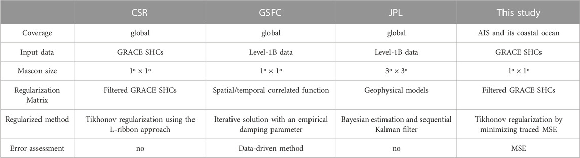
TABLE 2. Summary of the mascon solutions.

4 Results and discussion

4.1 Experimental design

4.1.1 Mascon set-up

The outlines of AIS and its 27 drainage basins defined by Zwally et al. (2012) are shown in Figure 2, where West Antarctic Ice Sheet (WAIS; Basins 1 and 18–23), East Antarctic Ice Sheet (EAIS; Basins 2–17) and Antarctic Peninsula Ice Sheet (APIS; Basins 24–27) are the three commonly interested regions. The description of the basins including area, number of mascon and length of grounding line is shown in Table 3. Considering more dense GRACE observations in polar regions, 2024 mascons of $1°\times 1°$ equal-area are parameterized covering both AIS and its 600 km buffer zone, and the mascons over AIS are also shown in Figure 2. To solve the mascons, we generate 3,616 pseudo-observations distributed with $0.75°\times 0.75°$ equal-area at the satellite altitude covering AIS and its buffer zone. To recover the leaked signals while reducing the computational burden as possible, the buffer zone is set to twice GRACE natural resolution (i.e., 600 km).

FIGURE 2

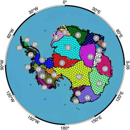
FIGURE 2. Regional distribution of basins (numbers 1–27) based on the definition of Zwally et al. (2012) and the distribution of mascon points covering AIS.

TABLE 3

TABLE 3. Description of the basins over AIS.

4.1.2 Construction of regularization matrix and determination of regularization parameter

To derive the signal variance (or RMS) of each mascon, we filter the Tongji-Grace2018 model by using the P4M6 decorrelation (Swenson and Wahr, 2006) and Gaussian smoothing (Wahr et al., 1998) with a radius of 100 km and 200 km, respectively. With the filtered Tongji-Grace2018 model from April 2002 to December 2016, we compute the RMS of each mascon that is then used to construct the regularization matrix. According to Save et al. (2016), the time variability of the regularization matrix is needed only for the larger river basins, hence a constant regularization matrix is used in our regional solution over AIS with the dominant signal of ice mass loss. The spatial distributions shown in Figure 3 are the RMS values derived from 100 km to 200 km Gaussian smoothing radius over AIS and 4 cm RMS over the buffer zone (Save et al., 2016), where the RMS values over the entire AIS present strong spatial heterogeneity and exceed 60 cm in the Amundsen Sea Embayment of the West Antarctic, much larger than that in the other regions. Additionally, the RMS values at Basins 18, 13, and parts of coastal EAIS (Basin 4–9) are moderate while that of the rest is relatively smaller. Compared to 100 km Gaussian smoothing, the signals derived from 200 km Gaussian smoothing have smaller RMS and more signal leakage.

FIGURE 3

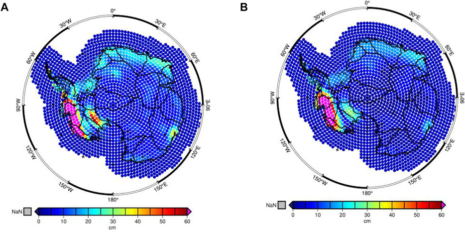
FIGURE 3. RMS of Gaussian 100 km + P4M6 (A) and Gaussian 200 km + P4M6 (B) filtered mass change from April 2002 to December 2016.

After the regularization matrix is constructed, the regularization parameter is determined by minimizing traced MSE and then the regularized solution is computed with Eq. 7. The regularization parameters of our solutions from April 2002 to December 2016 are shown in Figure 4. Since no seasonal variation exists in the regularization parameters, no unmodelled seasonal signals present in the residuals. Moreover, the regularization parameters in Figure 4 range from ${10}^{-8}$ to ${10}^{-6}$ and become larger before 2003 and after 2014 due to the worse quality of SHCs solutions.

FIGURE 4

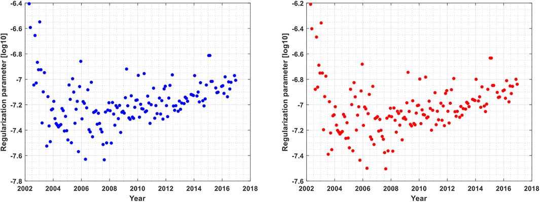
FIGURE 4. Regularization parameter with the prior information of RMS derived from the mass change signals with Gaussian 100 km + P4M6 (left) and Gaussian 200 km + P4M6 (right) filtering.

4.1.3 Mascon estimates with the regularization matrices from different prior information

To compare the filtered estimates by P4M6 and Gaussian smoothing with 100 km and 200 km radius with the correspondent mascon estimates with the regularization matrices constructed with the filtered estimates, we present in Figures 5A–D for the time series of mass change signals of the four estimates in Dronning Maud Land (DML), Kamb, Amundsen Sea Embayment (ASE) and APIS, where the two mascon estimates agree well and show more significant variations than the correspondent filtered estimates. After the time series of the four estimates are fitted with constant, trend, annual, semiannual and S₂ terms, the fitted signals of the mascon estimates are obviously stronger than those of the correspondent filtered estimates. The improvement ratio of the signal RMS values is defined as,

$\mathrm{i}\mathrm{m}\mathrm{p}\mathrm{r}\mathrm{o}\mathrm{v}\mathrm{e}\mathrm{m}\mathrm{e}\mathrm{n}\mathrm{t}\mathrm{r}\mathrm{a}\mathrm{t}\mathrm{i}\mathrm{o}=\frac{RMS\left(\mathrm{m}\mathrm{a}\mathrm{s}\mathrm{c}\mathrm{o}\mathrm{n}\right)-RMS\left(\mathrm{f}\mathrm{i}\mathrm{l}\mathrm{t}\mathrm{e}\mathrm{r}\right)}{RMS\left(\mathrm{f}\mathrm{i}\mathrm{l}\mathrm{t}\mathrm{e}\mathrm{r}\right)}*100\%$

FIGURE 5

FIGURE 5. Time series of mass change signals derived from two-step filtering (P4M6 and Gaussian smoothing with 100 km and 200 km radius) and the corresponding regularized mascon solutions. (A) DML (B) Kamb (C) ASE (D) APIS.

And the improvement ratios are presented in Table 4, in which the improvement ratios in ASE and APIS are 35.29% and 103.25% for the 100 km Gaussian filter, 53.81% and 116.86% for the 200 km Gaussian filter, respectively. In DML and Kamb, the improvement ratios are 21.65% and 14.07% for the 100 km Gaussian filter, and 38.07% and 70.41% for the 200 km Gaussian filter, respectively. These improvements confirm the capability of the presented mascon method in recovering the leakage signal over coastal AIS.

TABLE 4

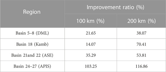
TABLE 4. Improvements for the mass change signals.

The mass change signals in June 2004 derived with P4M6 and Gaussian smoothing with 100 km and 200 km radius are shown in Figures 6A, B, and the correspondent mascon estimates are presented in Figures 6C, D, respectively. In Figure 6A, non-geophysical strips are still observable due to the 100 km weak filtering, while in Figure 6B 200 km moderate filtering leads to signal attenuation and leakage. Moreover, the mascon estimates in Figures 6C, D have higher spatial resolution and less signal leakage than their counterparts in Figures 6A, B. In detail, the mass loss signals over Basin 18 are clear in two mascon estimates and the mass gain over WAIS is also concentrated on the coast of WAIS in June 2004, which means that the spatial resolution is improved via the presented mascon method. Additionally, the mass change signals of our regularized mascon solutions in Figures 6C, D agree well with that of CSR and JPL mascon solutions in Figures 6E, F, much better than their filtering counterparts in Figures 6A, B. Therefore, our mascon solutions have obvious advantages in signal recovery compared to their filtering counterparts. The slight difference between Figures 6C, D is attributed to different prior information used in the regularization matrix, which means that prior information does affect the spatial resolution of mascon estimates. Therefore, the regularization matrix should be constructed carefully especially when a high-resolution solution is needed. Comparing Figures 6C, D, we find that the mascon estimates with the prior information from 100 km Gaussian filtering have a bit higher spatial resolution and better spatial patterns relative to the mascon estimates in Figures 6E, F than that from 200 km Gaussian filtering. Hence in the following sections, we derive our mascon solutions using the regularization matrix derived from 100 km Gaussian filtering.

FIGURE 6

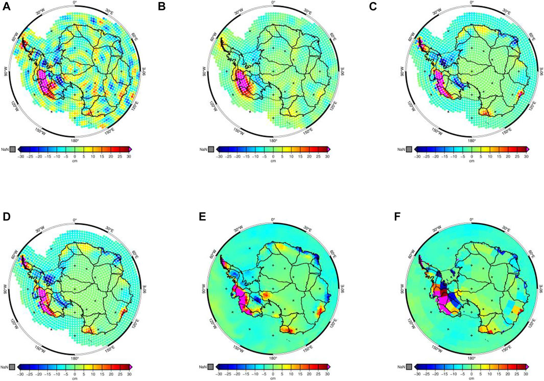
FIGURE 6. Mass change signals in June 2004. (A) and (B): P4M6 with Gaussian 100 and 200 km; (C) and (D): the correspondent mascon solutions; (E) and (F): CSR and JPL mascon solutions.

4.1.4 Error assessment of regularized mascon estimates

With the proposed regional mascon method, there are 157 months of mascon estimates are derived from April 2002 to December 2016, in which 20 months are missing, since the Tongji-Grace2018 model is not available during these months. In each estimate, 2024 mascons are estimated. Since the Tikhonov regularized estimates are biased, the biases must be taken into account when assessing the precisions of the estimates. Therefore, we use the MSE, which consists of covariance and squared biases, to assess the precisions of our mascon estimates. The average values of the MSE roots and absolute biases of 2024 mascon estimates are presented in Figure 7 for 157 months in terms of Gt. The mean absolute biases of the 2024 parameters range from 0.01 to 0.06 Gt with an average of 0.02 Gt, which are much smaller than the correspondent mean MSE roots that range from 0.10 to 0.17 Gt with an average of 0.13 Gt. Hence, the biases are well controlled in our regularized mascon solutions. The MSE roots of 157 months are shown in Figure 8 in terms of EWH for 2024 mascon estimates, where there are 1813 mascons (89.6%) with the mean MSE roots less than 2 cm and 13 mascons (0.64%) over 10 cm. And the large MSE roots appear on the coastline of the ASE in West Antarctic with a maximum value of 19.04 cm, where the signal variations are also very large with a maximum of 336.21 cm.

FIGURE 7

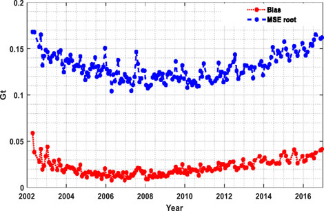
FIGURE 7. Mean absolute biases and MSE roots of 2024 mascons for 157 months in terms of Gt.

FIGURE 8

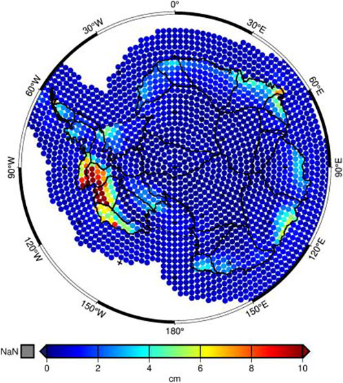
FIGURE 8. The mean MSE roots of 157 months for the 2024 mascons.

4.2 Experimental results

4.2.1 Characteristics of mass change signals over AIS

The summed time series of mass change signals over AIS from April 2002 to December 2016 of our regularized mascon solutions are presented in Figure 9, together with that of CSR (Save et al., 2016), GSFC (Loomis et al., 2019b), JPL (Watkins et al., 2015) and mascon with identity regularization matrix, where the AIS was close to a state of balance before 2007, but with a significant mass loss after 2008, which is consistent with the finding in Shepherd et al. (2018) and Loomis et al. (2019a); Loomis et al. (2020).

FIGURE 9

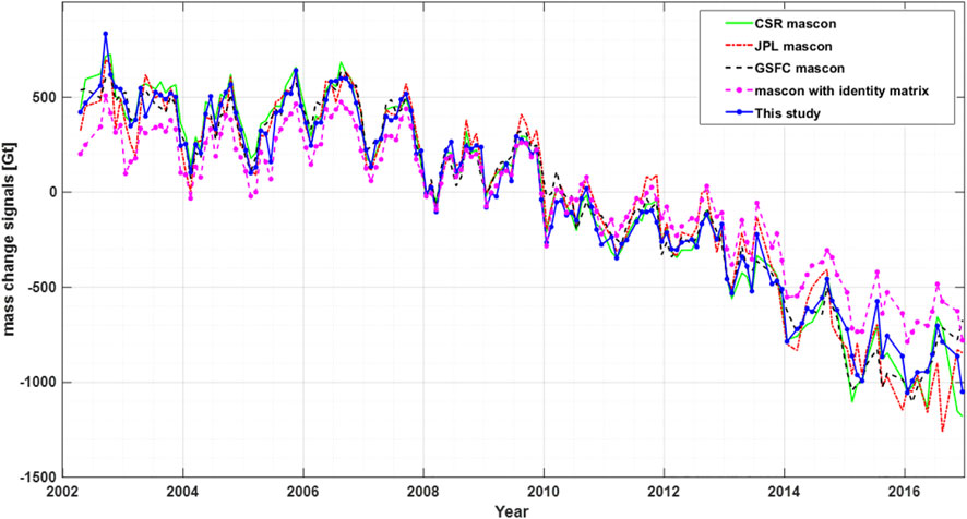
FIGURE 9. Time series of mass change signals over AIS from April 2002 to December 2016.

According to Loomis et al. (2019a); Loomis et al. (2020), five series in Figure 9 are divided into two periods (period-1 from April 2002 to June 2007 and period-2 from July 2007 to December 2016) and then fitted with constant, trend (rate), annual, semiannual and S₂ terms. The results of mass change rate, annual, and semiannual amplitudes are presented in Table 5, in which the uncertainties are at a 95% confidence level. The mass change rate of mascon with identity regularization matrix for the period from 2002 to 2016 is only −68.3 ± 5.1 Gt/yr due to large land-ocean leakage. For the same period, the mass change rate of our mascon solution is −103.6 ± 5.6 Gt/yr, consistent with the results of three global mascon solutions and −121.6 ± 14.7 Gt/yr from altimetry within the uncertainty (Shepherd et al., 2019). For the first period from April 2002 to June 2007, the mass change rate is very small and with large uncertainty, which is −17.4 ± 17.7 Gt/yr, while for the second period, the rate is −144.7 ± 7.3 Gt/yr, hence the ice mass loss became significant after 2007. As for the annual and semiannual amplitudes, the results from the five series are quite consistent within the uncertainty. From period-1 to period-2, the annual and semiannual amplitudes from our mascon solution diminished from 149.0 ± 36.6 Gt to 134.6 ± 28.0 Gt, and 52.94 ± 36.5 Gt to 26.8 ± 28.8 Gt, respectively.

TABLE 5

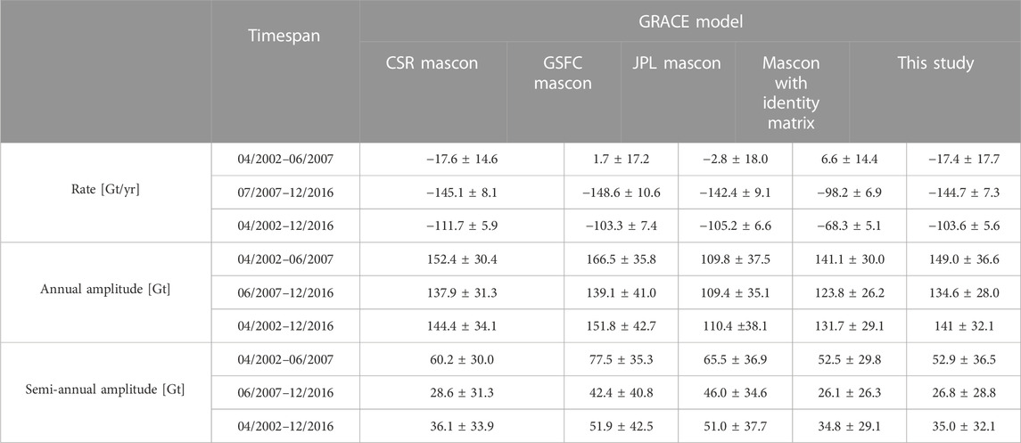
TABLE 5. Rate, annual amplitude and semi-amplitude of mass change signals over AIS.

The spatial patterns of mass change rates over AIS are shown in Figure 10 for period-1, period-2, and the whole study period.

FIGURE 10

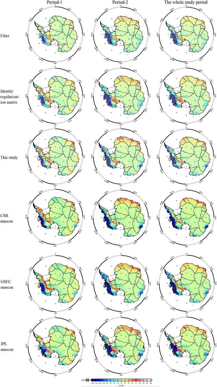
FIGURE 10. Spatial distribution of mass change rates over AIS from April 2002 to December 2016.

4.2.2 Mass change signals in EAIS, WAIS, APIS, and 27 basins

The time series of mass change signals over EAIS, WAIS and APIS are presented in Figure 11. We can observe from Figure 11 that EAIS experienced a slow rise before 2009, followed by an intensive rise during 2009–2012 and then a slow decline after 2013. As explained in Section 4, the intensified accumulation was caused by the sharp increasing snowfall between 2009 and 2012 (Boening et al., 2012; Shepherd et al., 2019). WAIS experienced a slow mass loss before 2008, an intense loss during 2009–2014, and a slow loss again after 2014. APIS experienced a steady mass loss from the middle of 2006 to the beginning of 2016, which is consistent with that in Figure 10 where the pattern over APIS in period-2 is significant while that in period-1 is not obvious. Overall, the three regions have quite different mass change characteristics. The estimated mass change rates over EAIS, WAIS and APIS from April 2002 to December 2016 are shown in Table 6, in which our solutions are consistent with CSR, GSFC, and JPL solutions within the uncertainties.

FIGURE 11

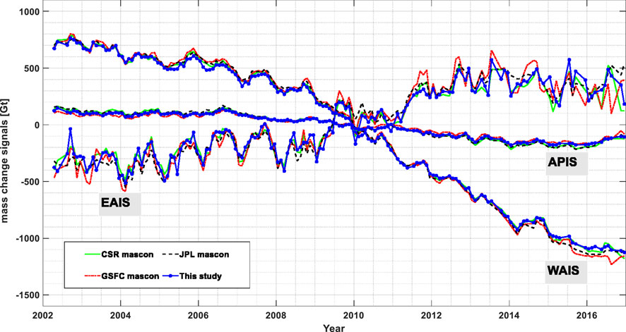
FIGURE 11. Time series of mass change signals over EAIS, WAIS and APIS from April 2002 to December 2016.

TABLE 6

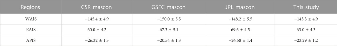
TABLE 6. Mass change rate from April 2002 to December 2016.

The mass change rates and annual amplitude at the basin scale are also estimated from the $1°\times 1°$ equal-area mascon estimates by the least-square fitting, and the results are shown in Figure 12, where APIS is the summed area of four small basins, that is Basins 24, 25, 26, and 27. The large mass gains are in Basins 7 and 18, with rates of 18.03 ± 1.88 Gt/yr and 14.55 ± 0.60 Gt/yr, while the high mass losses are in Basins 21 and 22, with rates of –58.57 ± 2.48 Gt/yr and –44.12 ± 2.27 Gt/yr. The rates in most basins of EAIS show good consistency between ours and those of CSR, GSFC and JPL. However, for the basins in WAIS (Basins 1, 20, 21, 22, and 23), the discrepancies in mass change rates between the four mascon solutions are relatively large. Especially for the rates in Basins 18, 20, and 21, the GSFC solution does not agree with the other three solutions within the error bars of 95% confidence level. The mass change rate from the JPL solution in basin 1 also does not agree with the other three solutions within the error bars. However, our regional solution agrees well with the CSR solution except for Basin 23, and in Basin 23 our solution agrees with the JPL solution. The estimated annual amplitudes agree well between the four mascon solutions within the error bars, except for Basins 3 and 18, in which, however, our solution still agrees with the CSR solution. The probable reason for the better agreement is that we use the same method as CSR to construct the regularization matrix.

FIGURE 12

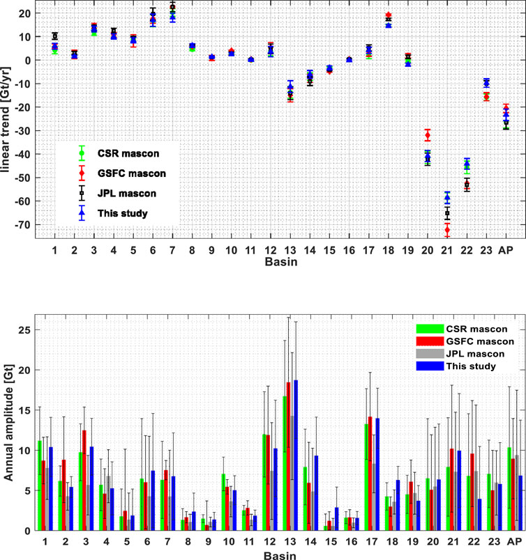
FIGURE 12. Mass change rates and annual amplitudes at a basin scale (with a 95% confidence level). AP denotes APIS.

4.3 Discussion

4.3.1 Spatial pattern comparison of mass change rate over AIS

As shown in Figure 10, compared to the results derived from P4M6 + Gaussian 200 km and the mascon solution with identity regularization matrix (the first and second rows of Figure 10), the mass change rates of our mascon solutions are more clear with stronger mass loss and gain signals. The maximum mass gain rate over the coast of Basin 7 in period-2 is over 16 cm/yr, while that of the filtered one and the mascon solution with identity regularization matrix is only 4 cm/yr and 8 cm/yr. Moreover, the mass loss rate in Totten glacier (Basin13) for period-2 is very significant, with an extreme value of over −16 cm/yr, while that of the filtered one and the mascon solution with identity regularization matrix is only −6 cm/yr and −7 cm/yr. Therefore, our mascon solutions can squeeze more signals than the correspondent filtering ones and the mascon solution with an identity regularization matrix. In general, the three global mascon solutions have more similar spatial patterns to our mascon solutions than the filtering ones. The mass change signals of our mascon solutions are also more coincident with the shape of glaciers and ice streams than that of the filtering ones, such as the most striking ice mass loss in Getz (Basin 20), Thwaites (Basin 21) and Pine Island (Basin 22), and the ice mass gain in Kamb Ice Stream (Basin 18), which are consistent with the findings in Rignot et al. (2011); Shepherd et al. (2019). Therefore, our mascon estimates with the higher spatial resolution are more reliable than the correspondent filtered estimates and the mascon solution with identity regularization matrix. Compared to GSFC and JPL mascon solutions, the mass gain rates in Basin 18 from our mascon and CSR mascon solutions are more coincident with that of the Kamb Ice Stream. And the mass loss rate in Totten glacier of Basin 13 is as well. As shown in the first two columns of Figure 10, the spatial patterns in the two periods are obviously different, the mass loss area in period-2 is much larger than that in period-1, especially in the coastline of the ASE of West Antarctic, which is consistent with the finding in Harig and Simons (2015). The mass loss rates in Totten and Moscow (basin 13), as well as in basin 15, are also enhanced. Interestingly, some regions have opposite mass change rates in the two periods. For instance, the western Dronning Maud Land (basins 5–6) experienced ice mass loss in period-1 and mass gain in period-2, which is consistent with Shepherd et al. (2019) who derived the results from satellite altimetry. In the whole Dronning Maud Land (basins 5–8), a broad pattern of modest ice sheet mass gain spans much of the coastline and stretches inland for several kilometers in the whole study period, which is associated with sharp increases in snowfall that happened from 2009 to 2012 (Boening et al., 2012; Shepherd et al., 2019).

4.3.2 Annual and interannual signals comparison with RACMO

To compare the annual and interannual signals of the four mascon solutions with the cumulated SMB from RACMO, the detrended and smoothed (with a 7-month moving average filter) time series of the mass change signals in EAIS, WAIS and APIS are shown in Figure 13 together with that from RACOM. The estimated RMSE (root mean squared error) values from the differences between the four mascon solutions relative to the cumulated SMB in Figure 13 are illustrated in Table 7 together with correlation coefficients between the time series of cumulated SMB and the four mascon solutions. Except for the GSFC solution in EAIS, all the correlation coefficients and RMSE values in Table 7 are close to each other and the correlation coefficients are at least equal to 0.91. The four mascon solutions have the same correlation coefficients in WAIS and APIS, however, the JPL solution has the highest correlation coefficient in EAIS, and our solution has the same correlation coefficient as the CSR solution. As for the RMSE values, our solution has the smallest value in EAIS, the CSR solution has the smallest value in WAIS and JPL solution is the smallest in APIS.

FIGURE 13

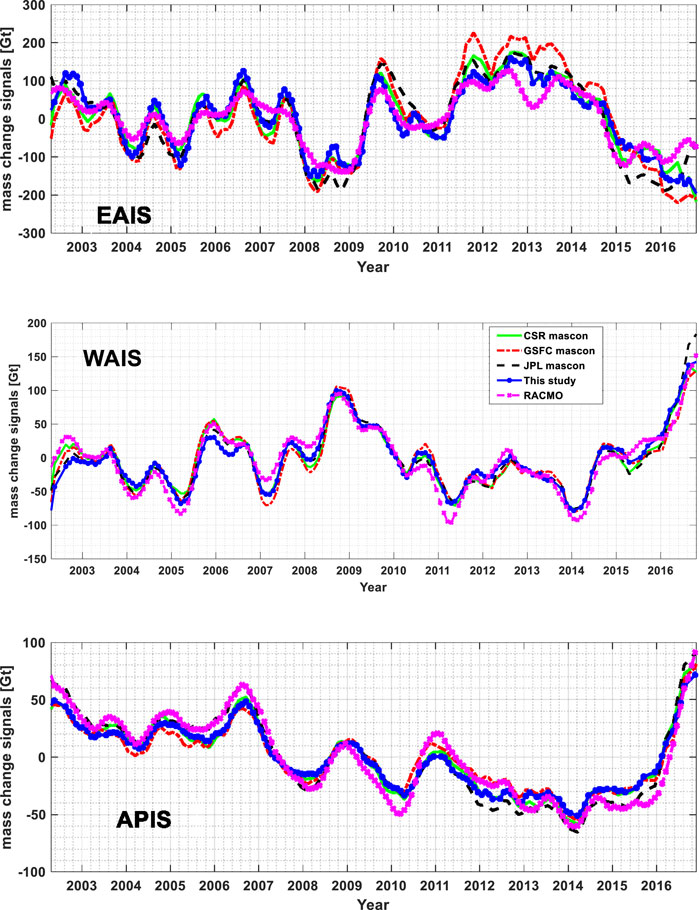
FIGURE 13. Detrend and smoothed mass change signals of four mascon solutions and cumulative SMB.

TABLE 7

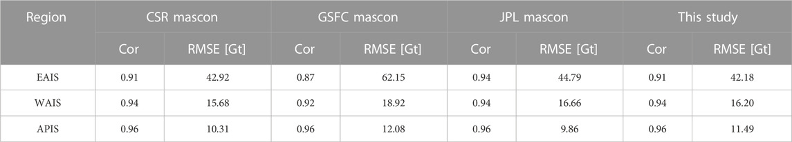
TABLE 7. Correlation coefficients and RMSE of detrended and smoothed mass change from four mascon solutions and RACMO.

After detrended and smoothed, more obvious annual variations can be observed in Figure 13 than that in Figure 11, and the discrepancies between the four mascon solutions are obviously smaller than that relative to cumulated SMB. By the way, due to the enhanced precipitation during the extreme 2015–2016 EL Niño (Bodart and Bingham, 2019), a significant mass gain in APIS and WAIS can be observed by the mascon solutions.

5 Conclusion

This contribution proposed the gravitational potential-based regional mascon method, in which the pseudo-observations of gravitational potential are generated from unfiltered GRACE level-2 data, and the regularization matrix is constructed with the prior information derived from the GRACE level-2 data with two-step filtering of 100 km radius. With the regional mascon method, the $1°\times 1°$ equal-area mascon solutions over AIS are derived from the Tongji-Grace2018 model from April 2002 to December 2016. The results demonstrate that our regional mascon solutions can achieve a better spatial resolution, and effectively reduce the land-ocean signal leakage and the signal leakage between the adjacent mascons.

The mass change signals of our mascon solutions have been significantly enhanced relative to the filtering counterparts with the improvement ratios of 21.65%, 14.07%, 35.29%, and 103.25% in DML, Kamb, ASE and APIS, which confirmed the capability of the presented regional mascon method in recovering the leakage signal over coastal AIS. The mass change rates over AIS of our mascon solution are −103.6 ± 5.6 Gt/yr from 2002 to 2016, –17.4 ± 17.7 Gt/yr during 2002–2007, and −144.7 ± 7.3 Gt/yr from 2008 to 2016, the ice mass loss is significantly intensified after 2007. In EAIS, WAIS, and APIS, the mass change rates from 2002 to 2016 are quite different, with the rates of 63.0 ± 4.3 Gt/yr, −143.3 ± 4.9 Gt/yr and −23.29 ± 1.2 Gt/yr respectively. The mass change signals at the basin scale with even more distinguishing features, significant mass gain occurred in Basins 7 and 18, with the rates of 18.03 ± 1.88 Gt/yr and 14.55 ± 0.60 Gt/yr, while large mass loss presented in Basins 21 and 22, with the rates of −58.57 ± 2.48 Gt/yr and −44.12 ± 2.27 Gt/yr. Relative to the cumulated SMB from RACMO, the correlation coefficients of four mascon solutions are at least equal to 0.91 except for the GSFC solution in EAIS.

Since the pseudo-observations are generated from GRACE level-2 data, the proposed regional mascon method has a lower computation burden and can be more easily optimized than the present global mascon methods. Moreover, the regional mascon method can achieve much better results than the filtered counterparts and its solutions are as good as the global mascon solutions, although the regularization matrix is simply constructed with the prior information from the filtered GRACE level-2 data in AIS and with the constant variance in the buffer zone. If the additional information from high-resolution global ocean and sea ice data synthesis, i.e., ECCO2 (Estimating the Circulation and Climate of the Ocean) or sea level change from satellite altimetry can be used to estimate the signal variances in the buffer zone, and the information from InSAR (Interferometric synthetic aperture radar) or ICESat (Ice, Cloud, and land Elevation Satellite) is used to refine the signal variances in AIS, the spatial resolution and the accuracy of the mascon solution are looking forwards to be further increased.

Data availability statement

The original contributions presented in the study are included in the article/supplementary material, further inquiries can be directed to the corresponding author.

Author contributions

WW performed the data processing, analyzed the experimental results, and drafted the manuscript. YS performed the methodology research, designed the study, conducted the analysis of the results and revised the manuscript. QC and TC checked the performance of this method and revised the manuscript. All authors read and approved the final manuscript.

Funding

This work is sponsored by the Natural Science Foundation of China (42274005 and 41974002).

Acknowledgments

We thank Prof. Jürgen Kusche for the discussion on the methodology and result analysis of this work. Dr. Melchior van Wessem is acknowledged for providing the RACMO2.3p2 SMB data. Last but not least, we appreciate the constructive comments from the two reviewers, which led to significant improvement of the manuscript.

Conflict of interest

The authors declare that the research was conducted in the absence of any commercial or financial relationships that could be construed as a potential conflict of interest.

Publisher’s note

All claims expressed in this article are solely those of the authors and do not necessarily represent those of their affiliated organizations, or those of the publisher, the editors and the reviewers. Any product that may be evaluated in this article, or claim that may be made by its manufacturer, is not guaranteed or endorsed by the publisher.

References

Barletta, V. R., Sørensen, L. S., and Forsberg, R. (2013). Scatter of mass changes estimates at basin scale for Greenland and Antarctica. Cryosphere 7 (5), 1411–1432. doi:10.5194/tc-7-1411-2013

CrossRef Full Text | Google Scholar

Baur, O., and Sneeuw, N. (2011). Assessing Greenland ice mass loss by means of point-mass modeling: A viable methodology. J. Geodesy 85 (9), 607–615. doi:10.1007/s00190-011-0463-1

CrossRef Full Text | Google Scholar

Bodart, J. A., and Bingham, R. J. (2019). The impact of the extreme 2015–2016 El Niño on the mass balance of the Antarctic ice sheet. Geophys. Res. Lett. 46, 13862–13871. doi:10.1029/2019GL084466

CrossRef Full Text | Google Scholar

Boening, C., Lebsock, M., Landerer, F., and Stephens, G. (2012). Snowfall-driven mass change on the East Antarctic ice sheet. Geophys. Res. Lett. 39, L21501. doi:10.1029/2012GL053316

CrossRef Full Text | Google Scholar

Chen, J., Wilson, C., Li, J., and Zhang, Z. (2015). Reducing leakage error in GRACE-observed long-term ice mass change: A case study in West Antarctica. J. Geodesy 89, 925–940. doi:10.1007/s00190-015-0824-2

CrossRef Full Text | Google Scholar

Chen, Q., Shen, Y., Chen, W., Francis, O., Zhang, X., Chen, Q., et al. (2019). An optimized short-arc approach: Methodology and application to develop refined time series of Tongji-Grace2018 GRACE monthly solutions. J. Geophys. Res. Solid Earth 124, 6010–6038. doi:10.1029/2018JB016596

CrossRef Full Text | Google Scholar

Chen, Q., Shen, Y., Kusche, J., Chen, W., Chen, T., and Zhang, X. (2021). High-resolution GRACE monthly spherical harmonic solutions. J. Geophys. Res. Solid Earth 126, e2019JB018892. doi:10.1029/2019JB018892

CrossRef Full Text | Google Scholar

Chen, T., Kusche, J., Shen, Y., and Chen, Q. (2020). A combined use of TSVD and Tikhonov regularization for mass flux solution in Tibetan plateau. Remote Sens. 12 (12), 2045. doi:10.3390/rs12122045

CrossRef Full Text | Google Scholar

Chen, T., Shen, Y., and Chen, Q. (2016). Mass flux solution in the Tibetan plateau using mascon modeling. Remote Sens. 8 (5), 439. doi:10.3390/rs8050439

CrossRef Full Text | Google Scholar

Ditmar, P. (2018). Conversion of time-varying Stokes coefficients into mass anomalies at the Earth’s surface considering the Earth’s oblateness. J. Geodesy 92, 1401–1412. doi:10.1007/s00190-018-1128-0

PubMed Abstract | CrossRef Full Text | Google Scholar

Dobslaw, H., Dill, R., Bagge, M., Klemann, V., Boergens, E., Thomas, M., et al. (2020). Gravitationally consistent mean barystatic sea level rise from leakage-corrected monthly GRACE data. J. Geophys. Res. Solid Earth 125, e2020JB020923. doi:10.1029/2020JB020923

CrossRef Full Text | Google Scholar

Forsberg, R., and Reeh, N. (2007). “Mass change of the Greenland ice sheet from GRACE,” in Proceedings of the 1st international symposium of IGFS, Harita Dergisi, 454–458.18

Google Scholar

Forsberg, R., Sørensen, L., and Simonsen, S. (2017). Greenland and Antarctica ice sheet mass changes and effects on global sea level. Germany: Springer International Publishing.

Google Scholar

Geruo, A., Wahr, J., and Zhong, S. (2013). Computations of the viscoelastic response of a 3-D compressible earth to surface loading: An application to glacial isostatic adjustment in Antarctica and Canada. Geophys. J. Int. 192 (2), 557–572. doi:10.1093/gji/ggs030

CrossRef Full Text | Google Scholar

Golub, G. M., Heath, M., and Wahba, G. (1979). Generalized cross-validation as a method for choosing a good ridge parameter. Technometrics 21, 215–223. doi:10.1080/00401706.1979.10489751

CrossRef Full Text | Google Scholar

Groh, A., and Horwath, M. (2021). Antarctic ice mass change products from GRACE/GRACE-FO using tailored sensitivity kernels. Remote Sens. 13, 1736. doi:10.3390/rs13091736

CrossRef Full Text | Google Scholar

Groh, A., Horwath, M., Horvath, A., Meister, R., Sørensen, L. S., Barletta, V. R., et al. (2019). Evaluating GRACE mass change time series for the antarctic and Greenland ice sheet—methods and results. Geosciences 9, 415. doi:10.3390/geosciences9100415

CrossRef Full Text | Google Scholar

Hansen, P. C., and O’Leary, D. P. (1993). The use of the L-curve in the regularization of discrete ill-posed problems. SIAM J. Comput. 14 (6), 1487–1503. doi:10.1137/0914086

CrossRef Full Text | Google Scholar

Harig, C., and Simons, F. J. (2015). Accelerated west Antarctic ice mass loss continues to outpace east Antarctic gains. Earth Planet. Sci. Lett. 415, 134–141. doi:10.1016/j.epsl.2015.01.029

CrossRef Full Text | Google Scholar

Harig, C., and Simons, F. J. (2012). Mapping Greenland's mass loss in space and time. PNAS 109 (49), 19934–19937. doi:10.1073/pnas.1206785109

PubMed Abstract | CrossRef Full Text | Google Scholar

Hoerl, A. E., and Kennard, R., W. (1970). Ridge regression: Biased estimation for nonorthogonal problems. Technometrics 12, 55–67. doi:10.1080/00401706.1970.10488634

CrossRef Full Text | Google Scholar

Ivins, E. R., James, T. S., Wahr, J., Schrama, O., Ernst, J., Landerer, F. W., et al. (2013). Antarctic contribution to sea level rise observed by GRACE with improved GIA correction. J. Geophys. Res. Solid Earth 118, 3126–3141. doi:10.1002/jgrb.50208

CrossRef Full Text | Google Scholar

Iz, H. B., Yang, T. Y., and Shum, C. K. (2021). The rigorous adjustment of the global mean sea level budget during 2005–2015. Geodesy Geodyn. 12, 175–180. doi:10.1016/j.geog.2020.03.001

CrossRef Full Text | Google Scholar

Jacob, T., Wahr, J., Pfeffer, W. T., and Swenson, S. (2012). Recent contributions of glaciers and ice caps to sea level rise. Nature 482 (7386), 514–518. doi:10.1038/nature10847

PubMed Abstract | CrossRef Full Text | Google Scholar

Jekeli, C. (1981). Alternative methods to smooth the Earth’s gravity field; report 327 of geodetic science and surveying. Columbus, OH, USA: Ohio Ohio State University.

Google Scholar

Jing, W., Zhang, P., and Zhao, X. (2019). A comparison of different GRACE solutions in terrestrial water storage trend estimation over Tibetan Plateau. Sci. Rep. 9, 1765. doi:10.1038/s41598-018-38337-1

PubMed Abstract | CrossRef Full Text | Google Scholar

Khan, S. A., Aschwanden, A., Bjørk, A. A., Wahr, J., Kjeldsen, K. K., and Kjaer, K. H. (2015). Greenland ice sheet mass balance: A review. Rep. Prog. Phys. 78 (4), 046801. doi:10.1088/0034-4885/78/4/046801

PubMed Abstract | CrossRef Full Text | Google Scholar

Koch, K-R., and Kusche, J. (2002). Regularization of geopotential determination from satellite data by variance components. J. Geodesy 76, 259–268. doi:10.1007/s00190-002-0245-x

CrossRef Full Text | Google Scholar

Kusche, J., Schmidt, R., Petrovic, S., and Rietbroek, R. (2009). Decorrelated GRACE time-variable gravity solutions by GFZ, and their validation using a hydrological model. J. Geodesy 83, 903–913. doi:10.1007/s00190-009-0308-3

CrossRef Full Text | Google Scholar

Li, J., Chen, J., Li, Z., Wang, S.-Y., and Hu, X. (2017). Ellipsoidal correction in GRACE surface mass change estimation. J. Geophys. Res. Solid Earth 122, 9437–9460. doi:10.1002/2017JB014033

CrossRef Full Text | Google Scholar

Loomis, B. D., Luthcke, S. B., and Sabaka, T. J. (2019b). Regularization and error characterization of GRACE mascons. J. Geodesy 93 (9), 1381–1398. doi:10.1007/s00190-019-01252-y

PubMed Abstract | CrossRef Full Text | Google Scholar

Loomis, B. D., Rachlin, K. E., and Luthcke, S. B. (2019a). Improved Earth oblateness rate reveals increased ice sheet losses and mass-driven sea level rise. Geophys. Res. Lett. 46, 6910–6917. doi:10.1029/2019GL082929

CrossRef Full Text | Google Scholar

Loomis, B. D., Rachlin, K. E., Wiese, D. N., Landerer, F. W., and Luthcke, S. B. (2020). Replacing GRACE/GRACE-FO with satellite laser ranging: Impacts on antarctic ice sheet mass change. Geophys. Res. Lett. 47, e2019GL085488. doi:10.1029/2019GL085488

CrossRef Full Text | Google Scholar

Mu, D. P., Yan, H. M., Feng, W., and Peng, P. (2017). GRACE leakage error correction with regularization technique: Case studies in Greenland and Antarctica. Geophys. J. Int. 208, ggw494–1786. doi:10.1093/gji/ggw494

CrossRef Full Text | Google Scholar

Nilsson, J., Vallelonga, P., Simonsen, S. B., Sorensen, L. S., Forsberg, R., Dahl-Jensen, D., et al. (2015). Greenland 2012 melt event effects on CryoSat-2 radar altimetry. Geophys. Res. Lett. 42, 3919–3926. doi:10.1002/2015GL063296

CrossRef Full Text | Google Scholar

Pattyn, F., Ritz, C., Hanna, E., Asay-Davis, X., DeConto, R., Durand, G., et al. (2018). The Greenland and Antarctic ice sheets under 1.5 °C global warming. Nat. Clim. Change 8 (12), 1053–1061. doi:10.1038/s41558-018-0305-8

CrossRef Full Text | Google Scholar

Peltier, W. R., Argus, D. F., and Drummond, R. (2018). Comment on “An Assessment of the ICE-6G_C (VM5a) Glacial Isostatic Adjustment Model” by Purcell et al. J. Geophys. Res. Solid Earth 123 (2), 2019–2028. doi:10.1002/2016JB013844

CrossRef Full Text | Google Scholar

Peltier, W. R. (2004). Global glacial isostasy and the surface of the ice-age Earth: The ICE-5G(VM2) model and GRACE. Annu. Rev. Earth Planet Sci. 32, 111–149. doi:10.1146/annurev.earth.32.082503.144359

CrossRef Full Text | Google Scholar

Ran, J. (2017). Analysis of mass variations in Greenland by a novel variant of the mascon approach. The Netherlands. doi:10.4233/uuid:cf99aded-77c9-42da-b0d4-009372620a2e

CrossRef Full Text | Google Scholar

Rignot, E., Mouginot, J., Scheuchl, B., Broeke, M., Wessem, M., and Morlighem, M. (2019). Inaugural article: Four decades of Antarctic ice sheet mass balance from 1979–2017. Proc. Natl. Acad. Sci. U. S. A. 116 (4), 1095–1103. doi:10.1073/pnas.1812883116

PubMed Abstract | CrossRef Full Text | Google Scholar

Rignot, E., Mouginot, J., and Scheuchl, B. (2011). Ice flow of the antarctic ice sheet. Science 333 (6048), 1427–1430. doi:10.1126/science.1208336

PubMed Abstract | CrossRef Full Text | Google Scholar

Riva, R. E., Gunter, B. C., Urban, T. J., Vermeersen, B. L., Lindenbergh, R. C., Helsen, M. M., et al. (2009). Glacial isostatic adjustment over Antarctica from combined ICESat and GRACE satellite data. Earth Planet. Sci. Lett. 288 (3), 516–523. doi:10.1016/j.epsl.2009.10.013

CrossRef Full Text | Google Scholar

Sasgen, I., Martín-Español, A., Horvath, A., Klemann, V., Petrie, E. J., Wouters, B., et al. (2017). Joint inversion estimate of regional glacial isostatic adjustment in Antarctica considering a lateral varying Earth structure (ESA STSE Project REGINA). Geophys. J. Int. 211, 1534–1553. doi:10.1093/gji/ggx368

CrossRef Full Text | Google Scholar

Sasgen, I., Martinec, Z., and Bamber, J. L. (2010). Combined GRACE and InSAR estimate of West Antarctic ice mass loss. J. Geophys. Res. Earth Surf. 115, F04010. doi:10.1029/2009JF001525

CrossRef Full Text | Google Scholar

Save, H., Bettadpur, S., and Tapley, B. D. (2016). High resolution CSR GRACE RL05 mascons. J. Geophys. Res. Solid Earth 121, 7547–7569. doi:10.1002/2016JB013007

CrossRef Full Text | Google Scholar

Save, H., Bettadpur, S., and Tapley, B. D. (2012). Reducing errors in the GRACE gravity solutions using regularization. J. Geodesy 86, 695–711. doi:10.1007/s00190-012-0548-5

CrossRef Full Text | Google Scholar

Scanlon, B. R., Zhang, Z., Save, H., Wiese, D. N., Landerer, F. W., Long, D., et al. (2016). Global evaluation of new GRACE mascon products for hydrologic applications. Water Resour. Res. 52, 9412–9429. doi:10.1002/2016wr019494

CrossRef Full Text | Google Scholar

Schrama, E. J. O., and Wouters, B. (2011). Revisiting Greenland ice sheet mass loss observed by GRACE. J. Geophys. Res. Solid Earth 116 (2), B02407. doi:10.1029/2009JB006847

CrossRef Full Text | Google Scholar

Schrama, E. J. O., Wouters, B., and Rietbroek, R. (2014). A mascon approach to assess ice sheet and glacier mass balances and their uncertainties from GRACE data. J. Geophys. Res. Solid Earth 119 (7), 6048–6066. doi:10.1002/2013JB010923

CrossRef Full Text | Google Scholar

Shen, Y., Xu, P., and Li, B. (2012). Bias-corrected regularized solution to inverse ill-posed models. J. Geodesy 86 (8), 597–608. doi:10.1007/s00190-012-0542-y

CrossRef Full Text | Google Scholar

Shepherd, A., Gilbert, L., Muir, A. S., Konrad, H., McMillan, M., Slater, T., et al. (2019). Trends in antarctic ice sheet elevation and mass. Geophys. Res. Lett. 46, 8174–8183. doi:10.1029/2019GL082182

PubMed Abstract | CrossRef Full Text | Google Scholar

Shepherd, A., Ivins, E., Rignot, E., Smith, B., van den Broeke, M., Velicogna, I., et al. (2018). Mass balance of the antarctic ice sheet from 1992 to 2017. Nature 558 (7709), 219–222. doi:10.1038/s41586-018-0179-y

PubMed Abstract | CrossRef Full Text | Google Scholar

Sørensen, L. S., and Forsberg, R. (2010). Greenland ice sheet mass loss from GRACE monthly models, gravity. Geoid Earth Obs. 135, 527–532. doi:10.1007/978-3-642-10634-7_70

CrossRef Full Text | Google Scholar

Su, Y., Zheng, W., Yu, B., You, W., Yu, B., Xiao, D., et al. (2019). Surface mass distribution derived from three-dimensional acceleration point-mass modeling approach with spatial constraint methods. Chin. J. Geophys. 62 (2), 508–519. (in Chinese). doi:10.6038/CJG2019l0770

CrossRef Full Text | Google Scholar

Sun, Y., Riva, R., and Ditmar, P. (2016). Optimizing estimates of annual variations and trends in geocenter motion and J2 from a combination of GRACE data and geophysical models. J. Geophys. Res. Solid Earth 121, 8352–8370. doi:10.1002/2016JB013073

CrossRef Full Text | Google Scholar

Swenson, S., Chambers, D., and Wahr, J. (2008). Estimating geo-center variations from a combination of GRACE and ocean model output. J. Geophys. Res. Solid Earth 113 (8), B08410. doi:10.1029/2007JB005338

CrossRef Full Text | Google Scholar

Swenson, S., and Wahr, J. (2006). Post-processing removal of correlated errors in grace data. Geophys. Res. Lett. 33 (8), L08402. doi:10.1029/2005gl025285

CrossRef Full Text | Google Scholar

Tapley, B. D., Watkins, M. M., Flechtner, F., Reigber, C., Bettadpur, S., Rodell, M., et al. (2019). Contributions of grace to understanding climate change. Nat. Clim. Change 9, 358–369. doi:10.1038/s41558-019-0456-2

PubMed Abstract | CrossRef Full Text | Google Scholar

Tikhonov, A. (1963). Solution of incorrectly formulated problems and the regularization method. Sov. Math. Dokl. 5, 1035–1038.

Google Scholar

Uebbing, B., Kusche, J., Rietbroek, R., and Landerer, F. W. (2019). Processing choices affect ocean mass estimates from GRACE. J. Geophys. Res. Oceans 124, 1029–1044. doi:10.1029/2018JC014341

CrossRef Full Text | Google Scholar

Undén, P., Rontu, L., Jarvinen, H., Lynch, P., Calvo, J., Cats, G., et al. (2002). HIRLAM-5 scientific documentation, Tech. Rep. December, Swedish Meteorology 35 and Hydrology Institute.

Google Scholar

van Wessem, J. M., Jan Van De Berg, W., Noël, B. P., Van Meijgaard, E., Amory, C., Birnbaum, G., et al. (2018). Modelling the climate and surface mass balance of polar ice sheets using RACMO2: Part 2: Antarctica (1979–2016). Cryosphere 12 (4), 1479–1498. doi:10.5194/tc-12-1479-2018

CrossRef Full Text | Google Scholar

van Wessem, J., Reijmer, C., Morlighem, M., Mouginot, J., Rignot, E., Medley, B., et al. (2014). Improved representation of East Antarctic surface mass balance in a regional atmospheric climate model. J. Glaciol. 60 (222), 761–770. doi:10.3189/2014jog14j051

CrossRef Full Text | Google Scholar

Vaughan, D. G., Comiso, J., and Allison, I. (2013). Observations: Cryosphere. Climate change 2013: The physical science basis. Contribution of working group I to the fifth assessment report of the intergovernmental panel on climate change. Retrieved from https://nyu-staging.pure.elsevier.com/en/publications/observations-cryosphere.

Google Scholar

Velicogna, I., Mohajerani, Y., Geruo, A., Landerer, F., Mouginot, J., Noel, B., et al. (2020). Continuity of ice sheet mass loss in Greenland and Antarctica from the GRACE and GRACE Follow-On missions. Geophys. Res. Lett. 47, e2020GL087291. doi:10.1029/2020GL087291

CrossRef Full Text | Google Scholar

Velicogna, I., Sutterley, T., and van den Broeke, M. (2014). Regional acceleration in ice mass loss from Greenland and Antarctica using GRACE time-variable gravity data. Geophys. Res. Lett. 41, 8130–8137. doi:10.1002/2014GL061052

CrossRef Full Text | Google Scholar

Velicogna, I., and Wahr, J. (2006). Measurements of time-variable gravity show mass loss in Antarctica. Science 311 (5768), 1754–1756. doi:10.1126/science.1123785

PubMed Abstract | CrossRef Full Text | Google Scholar

Velicogna, I., and Wahr, J. (2013). Time-variable gravity observations of ice sheet mass balance: Precision and limitations of the GRACE satellite data. Geophys. Res. Lett. 40, 3055–3063. doi:10.1002/grl.50527

CrossRef Full Text | Google Scholar

Wahr, J., Molenaar, M., and Bryan., F. (1998). Time variability of the Earth's gravity field: Hydrological and oceanic effects and their possible detection using GRACE. J. Geophys. Res. Solid Earth 103 (B12), 30205–30229. doi:10.1029/98jb02844

CrossRef Full Text | Google Scholar

Wahr, J., Swenson, S., and Velicogna, I. (2006). Accuracy of GRACE mass estimates. Geophys. Res. Lett. 33, L06401. doi:10.1029/2005GL025305

CrossRef Full Text | Google Scholar

Watkins, M. M., Wiese, D. N., Yuan, D.-N., Boening, C., and Landerer, F. W. (2015). Improved methods for observing Earth’s time variable mass distribution with GRACE using spherical cap mascons. J. Geophys. Res. Solid Earth 120, 2648–2671. doi:10.1002/2014JB011547

CrossRef Full Text | Google Scholar

Whitehouse, P., Bentley, M., Milne, G., King, M. A., and Thomas, I. D. (2012). A new glacial isostatic adjustment model for Antarctica: Calibrated and tested using observations of relative sea-level change and present-day uplift rates. Geophys. J. Int. 190 (2), 1464–1482. doi:10.1111/j.1365-246x.2012.05557.x

CrossRef Full Text | Google Scholar

Willen, M., Uebbing, B., and Horwath, M. (2018). Investigation of empirically estimated GIA over Antarctica based on various data inputs. Geophys. Res. Abstr. 20, EGU2018.

Google Scholar

Xu, P. (1992). Determination of surface gravity anomalies using gradiometric observables. Geophys. J. Int. 110, 321–332. doi:10.1111/j.1365-246x.1992.tb00877.x

CrossRef Full Text | Google Scholar

Xu, P. (1998). Truncated SVD methods for discrete linear ill-posed problems. Geophys. J. Int. 135, 505–514. doi:10.1046/j.1365-246x.1998.00652.x

CrossRef Full Text | Google Scholar

Yi, S., and Sun, W. (2014). Evaluation of glacier changes in high-mountain Asia based on 10 year GRACE RL05 models. J. Geophys. Res. Solid Earth 119, 2504–2517. doi:10.1002/2013JB010860

CrossRef Full Text | Google Scholar

Zhang, L., Yi, S., Wang, Q., Chang, L., Tang, H., and Sun, W. (2019). Evaluation of GRACE mascon solutions for small spatial scales and localized mass sources. Geophys. J. Int. 218, 1307–1321. doi:10.1093/gji/ggz198

CrossRef Full Text | Google Scholar

Zou, F., Tenzer, R., and Rathnayake, S. (2019). Monitoring changes of the antarctic ice sheet by GRACE, ICESat and GNSS. Contributions Geophys. Geodesy 49 (4), 403–424. doi:10.2478/congeo-2019-0021

CrossRef Full Text | Google Scholar

Zwally, H., Giovinetto, M., Beckley, M., and Saba, J. (2012). Antarctic and Greenland drainage systems. Available online: http://icesat4.gsfc.nasa.gov/cryo_data/ant_grn_drainage_systems.php

Google Scholar