Correlation between small earthquakes and CO2 anomalies in spring waters: a statistical experiment on the probability of seismic occurrence

We correlated carbon dioxide (${CO}_2$) time series detected at the Gallicano site in Tuscany, Italy, with low-magnitude earthquakes occurred in the surrounding area between 2017 and 2021. The ${CO}_2$ irregular component distribution was analyzed by a Pearson type VII fit, and its cumulate probability by the Gauss’s hypergeometric function, to statistically evidence anomalous fluctuations. We calculated the Matthews correlation between gas concentrations and low-magnitude earthquakes by defining a binary occurrence of ${CO}_2$ anomalies and seismic events. A positive correlation was highlighted by a time lag between the digital series, which resulted in ${CO}_2$ anomaly detections ahead of the earthquake time of two days. The correlated earthquakes were mainshocks of local magnitude 1.2 to 3.6, with epicenters within 40 $km$ from the Gallicano site. Correlations among rainfalls, ${CO}_2$ concentrations and earthquakes were also considered, showing that only few rainfall events were followed by a ${CO}_2$ anomaly, mostly a day late.

1 Introduction

The circulation of crustal fluids affects not only the transport of heat and chemical constituents, but also the mechanical processes that control rock deformation, and possibly generate earthquakes. Abnormal pressures in tectonically active areas were first reported by Anderson (1927), and overpressurized fluids were later identified as a primary agent of tectonic deformation by Hubbert and Rubey (1959). The observation of anomalous soil ${CO}_2$ concentrations in correspondence with major faults/fractured areas (Caucasus region; Netreba et al., 1971), and of ${CO}_2$ degassing episodes after major seismic events (Gold, 1979; Gold and Soter, 1979; Gold and Soter, 1981) dates back to early 1970s’. Based on a worldwide compilation of data, it has been later established that crustal ${CO}_2$ predominantly discharges in tectonically active regions, and along major seismic zones (Barnes et al., 1978; Irwin and Barnes, 1980; Gold and Soter, 1985; Gold, 1999). The occurrence of ${CO}_2$ emissions in correspondence with principal zones of seismicity was recently observed whether during the preparation stages of major earthquakes (e.g., among many others, Kingsley, 2001; Bräuer et al., 2003), or during aftershock evolutions (Ventura et al., 2007; Massin et al., 2013; Miller, 2013; Fischer et al., 2017; Yoshida and Hasegawa, 2018; Chiodini et al., 2020), or in concomitance with small seismic events (Heinicke et al., 1995). ${CO}_2$ excesses are predominantly observed in extensional domains (Tamburello et al., 2018), whereas compressional tectonic structures are suspected to create geological traps where crustal ${CO}_2$ may accumulate, possibly creating overpressurized reservoirs that may have the potential to trigger earthquakes (Chiodini et al., 2004). Overall, a strong connection between ${CO}_2$ discharge, seismic activity, and the existence of major faults has been identified in a number of different geodynamic contexts (Lee et al., 2016; Hunt et al., 2017).

In Central Italy, due to intense crustal deformation processes driven by the relative motion of the African and the Eurasian plates, two major areas affected by different tectonic and ${CO}_2$ degassing regimes have been identified (Chiodini et al., 2004): 1) the Tyrrhenian hinterland, characterized by extensional tectonic, crustal thinning, high heat flux and active volcanism near the Tyrrhenian Sea, where ${CO}_2$ is directly released into the atmosphere by the Tuscan-Roman and Campanian degassing structures; 2) the Adriatic foreland, characterized by compressional tectonics, where ${CO}_2$ is predominantly dissolved into groundwaters circulating through major carbonate aquifers hosted along the Apennine fold-and-thrust belt.

The central-southern part of Apennines is a highly active seismic area, and some authors (e.g., Chiodini et al., 2004; 2020) have speculated that the existence of high-pressure, ${CO}_2$-rich fluid pockets at depth may play a major role in the generation of Apennine earthquakes.

Since early 1990s’, a large amount of information on the possible correlation between ${CO}_2$ degassing and seismic activity has been obtained in Italy using manual samplings techniques (Dall’Aglio et al., 1990; Di Bello et al., 1998; Italiano et al., 2001; Italiano et al., 2004; Cardellini et al., 2017; Giudicepietro et al., 2019; Chiodini et al., 2020; Martinelli et al., 2020). The collection of continuous time series by means of automatic ground-based stations has started more recently (Cioni et al., 2007; Heinicke et al., 2012; Di Martino et al., 2013; Pering et al., 2014; Pierotti et al., 2015; Camarda et al., 2016; Camarda et al., 2018; Pierotti et al., 2017; Gherardi and Pierotti, 2018), and since early 2003 a network of six automatic monitoring stations is operating in Tuscany, Central Italy (Geochemical Monitoring Network of Tuscany, GMNT; Figure 1).

FIGURE 1

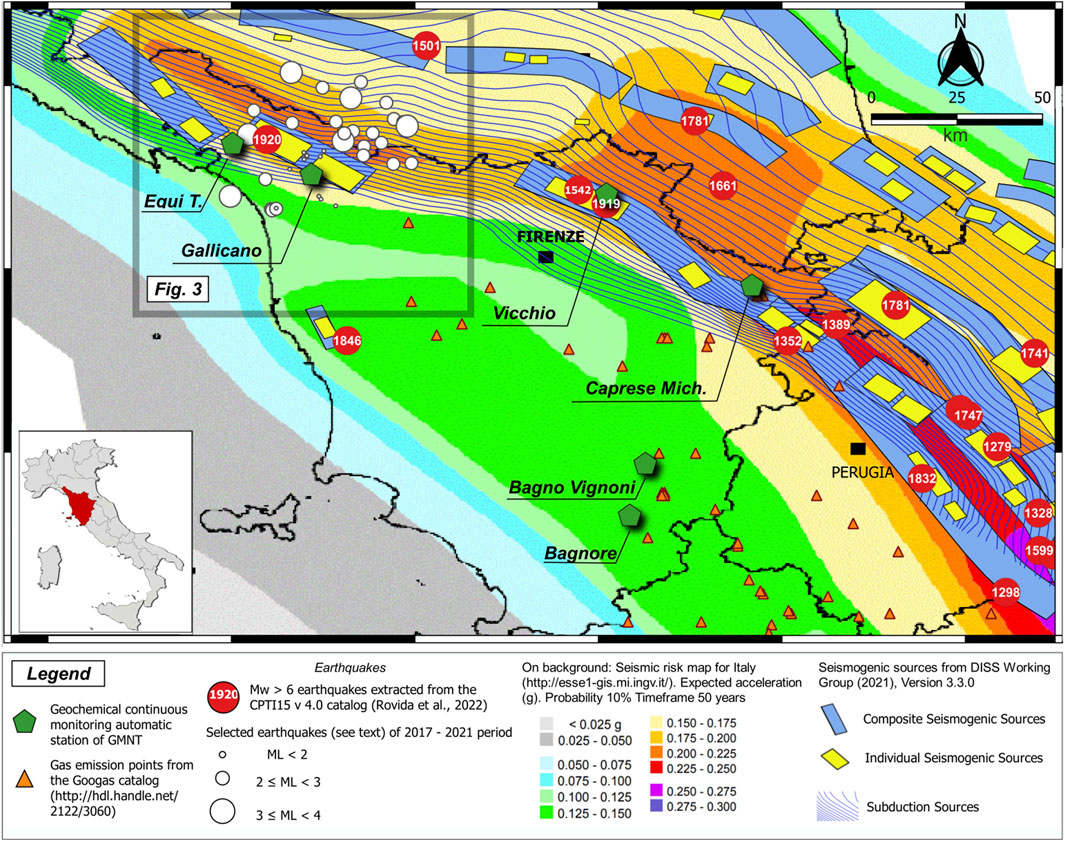
FIGURE 1. Location of the Gallicano monitoring station and other sites of the GMNT. The tectonic background and the epicenters of relevant seismic events are also shown.

Here we report on ${CO}_2$ time series collected during the 2017–2021 period from one of the stations of the GMNT (Gallicano station, NW Tuscany), advancing a new statistical interpretative approach borrowed from satellite data processing procedures (Fidani, 2021). So far, in fact, Gallicano time series have been processed with the aim to identify possible anomalies merely related to most energetic seismic events ($M_w$ > 4; e.g., Pierotti et al., 2015). Now, instead, the focus is on the possible correlation between low to moderate seismic events, which are inherently more numerous, and geochemical anomalies identified in the residuals of the ${CO}_2$ continually recorded signal. The proposed statistical approach allows for identifying ${CO}_2$ anomalies by cumulative probability, and for correlating them with earthquakes, without explicitly addressing the cause-effect mechanisms between the two classes of observable events. Finally, a conditional probability of earthquake occurrence is defined for possible short-term forecasting. At this stage, for ease of interpretation of the correlations, we focused solely on the geochemical signal of the Gallicano monitoring station, which has proven to be sensitive to crustal deformations (Pierotti et al., 2015). Future work will improve on this by extending the approach to the analysis of multiple geochemical time series collected from different monitoring stations, insofar as they are geologically linked to the same seismogenic structures.

2 Description of the study area

2.1 The Gallicano site

By discharging high-salinity Na-Ca-Cl waters (2.4 to 4.2 $g/L$), with a temperature of 23.4°C–25.2°C, and an average flow rate of about 1.5 $L/s$, the Gallicano thermomineral spring (209 m a.s.l., Garfagnana Valley, northern Tuscany, Italy), is considered a suitable site to investigate possible correlations between seismic events and anomalies in ${CO}_2$ dissolved concentrations (Cioni et al., 2007; Pierotti et al., 2015). Garfagnana Valley is one of the areas with the highest seismic risks in Tuscany. The region was struck by a $M_w$ 6.5 earthquake in 1920 (Garfagnana earthquake; Rovida et al., 2022), and is characterized by an expected horizontal peak ground acceleration (PGA) higher than 0.175 g, with a 10% probability of exceedance in 50 years (national reference seismic hazard model; Stucchi et al., 2011). The Gallicano thermomineral spring is fed by a major, fractured carbonate aquifer. After long underground circulation paths, thermal waters emerge in correspondence with neotectonic structures (Molli et al., 2021) belonging to one of the seismogenic boxes identified by the DISS Working group (2021). Chemical and isotopic data indicate that during their underground circulation path, Gallicano waters interact with evaporitic rocks of Triassic age, and experience the inflow of deep-seated ${CO}_2$ (Pierotti et al., 2015). These conditions reflect the essential criteria required for the successful monitoring of preseismic gas-geochemical signals (Martinelli and Albarello, 1997; King et al., 2006; Weinlich et al., 2006; Martinelli and Dadomo, 2017). Since April 2003, the spring is continuously monitored for a number of parameters, which include water temperature, pH, electrical conductivity, redox potential, and dissolved concentration of ${CO}_2$ and ${CH}_4$. Full details on the setup, operating mode, sensor technology, and performance of the automatic station are given by Pierotti et al. (2015).

2.2 Meteorological data

Operative since 2000, the automatic meteorological station of Gallicano (179 m.a.s.l., 44.064° Latitude North, and 10.443° Longitude East) is part of a regional network of about 440 manual and 133 automatic stations (Agro-Metereological Network) managed by the Regional Hydrological Service (SIR) of Tuscany. The station is located in the municipality of Gallicano, some 800 m ENE of the monitored spring, and acquires meteorological data every 5 min. 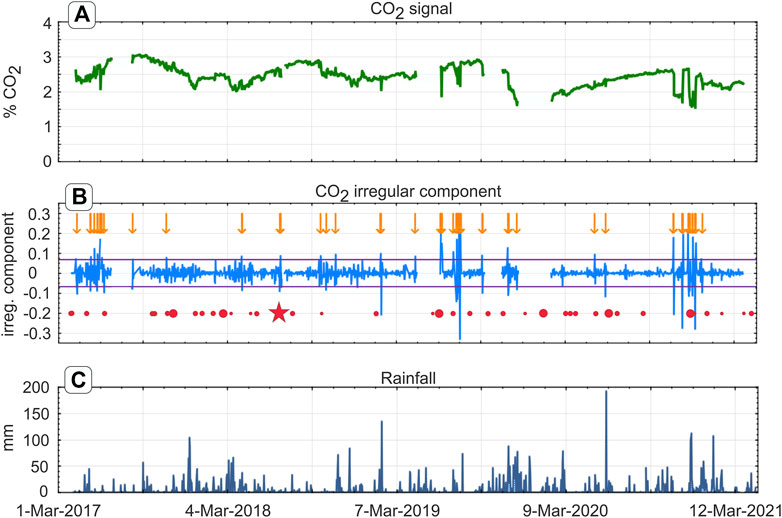Rainfall data for the period April 2017 to March 2021 are characterized by an average annual value of 1732 $mm/yr$, consistent with the average annual value of about 1880 $mm/yr$ estimated for the preceding period without data loss 2011–2016 (https://www.sir.toscana.it/pluviometria-pub). The two most abundant events recorded during the period of interest occurred on 2 February 2019 (134.8 $mm$) and 23 January 2021 (106.6 $mm$).

3 Methods

3.1 ${\mathit{C}\mathit{O}}_2$ monitoring

${CO}_2$ concentrations are measured with a specifically designed cell built in the Pisa laboratories of CNR-IGG (Cioni et al., 2007). The apparatus relies on the measurement of variations in $P_{CO2}$ within the cell, with $P_{CO2}$ values expressed as percent of the total pressure. The measure is done with an IR spectrophotomer operating over the analytical range 0%–10%, with an accuracy better than ± 2% of the range. Chemical speciation calculations and salting out corrections are used to periodically verify the response of the apparatus, by exploiting Henry’s law to relate carbon dioxide partial pressure ($P_{CO2}$) values measured in the cell to aqueous concentration (${CO}_{2\left(aq\right)}$) measured in water samples. In this contribution, we focus on ${CO}_2$ time series acquired during the 2017–2021 period. We processed raw data with appropriate moving median smoothing procedures (Box and Jenkins, 1976; Velleman and Hoaglin, 1981) to filter out a number of outliers recorded during monthly maintenance operations. The moving-median smoothing approach was preferred to the moving-average smoothing because of its superior ability to reduce the impact of the outliers present in the smoothing window. Our protocol considers a standard maintenance activity that includes monthly inspection of the whole apparatus, with an interruption of about one hour of the spring water supply to the measurement equipment. Therefore, in order to eliminate the outliers due to maintenance operations without affecting the signal, we applied a moving median smoothing window of $2N+1=25$ points. Following Pierotti et al. (2015), ${CO}_2$ time series have been decomposed according to Census I method (Makridakis et al., 1998) to detrend the ${CO}_2$ signal for external influences. In particular, according to Census technique, we polished the original time series for seasonal and cyclical components (combined with the additive model) to separate a residual component called “irregular component” (Figure 2). The decomposition was performed following a step-by-step procedure that considered a reference frame of 12 months (Makridakis et al., 1998). By definition, the irregular component of the ${CO}_2$ time series is the residual ${CO}_2$ time series resulting from non-systematic, short-term fluctuations, and corresponds to the high-frequency fluctuations of the series.

FIGURE 2

FIGURE 2. (A) ${CO}_2$ signal in vol.% of the headspace of the measurement cell; Cioni et al., 2007; Pierotti et al., 2015) acquired during the period April 2017–March 2021. (B) Irregular component of ${CO}_2$ time series, obtained by application of the Census I method. Purple lines represent the threshold for anomalous values (values outside this range have 99% probability of not belonging to a Pearson distribution). Orange arrows and red dots mark sixty-one (61) selected ${CO}_2$ anomalies and forty-two (42) selected seismic events (see text), respectively. Dots dimensions progressively increase with local magnitude ($M_L$). Seismic events are ranked into three classes of magnitude: low- ($M_L$ <2), intermediate- (2≤ $M_L$ <3), and high-energy events ($M_L$ ≥3). The most energetic event of 7 January 2018 ($M_L$ 3.6) is indicated by a red star. (C) rainfall at the Gallicano pluviometric station (data from https://www.sir.toscana.it/pluviometria-pub).

3.2 Earthquake declustering

We downloaded earthquake data from the catalog of the ISIDe Working Group (Italian Seismological Instrumental and parametric database; http://iside.rm.ingv.it) to obtain a subset of “significant events” with magnitude greater or equal to 1.0. The set was declustered using the Reasemberg (1985); Gardner and Knopoff (1974) methods, as implemented in the zmap suite of Matlab tools (Wiemer, 2001). The focus was on the low seismicity period between 19 March 2017, to 18 April 2021. During this period, we identified 785 seismic events within a radius of 50 km from the Gallicano site, and a maximum hypocentral depth of 50 km. The estimated magnitude of completeness was 1.4 (Figures 3A, B), and the greatest observed local magnitude $M_L=3.6$ (1 July 2018; epicenter near Pievepelago, about 700 m elevation, Modena Province). The areal distribution of seismicity is shown in Figure 3A, along with the traces of the main faults around the Gallicano site, whereas the distribution of hypocentral depths is shown in Figure 3C. Meteorological data were retrieved from the web archive of the Gallicano pluviometric station (https://www.sir.toscana.it/pluviometria-pub).

FIGURE 3

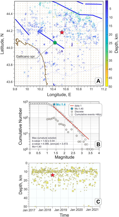
FIGURE 3. (A) Declustered earthquake dataset (785 declustered events of 3402 seismic events registered during the period), before further reduction for correlation analysis (42 seismic events after reduction). Brown line: Tyrrhenian coastline; blue line: main local faults; green pentagon: location of the Gallicano monitoring station. Dimensions and colors of square symbols indicate earthquakes magnitudes and depths, respectively, while the red star marks the most energetic seismic event occurred in the period of interest. (B) frequency-magnitude distribution. (C) earthquakes depth distribution (overall dataset, before processing).

3.3 Statistical treatment

The identification of ${CO}_2$ anomalies from the irregular dataset was realized with a standard step-by-step method. First, we fitted the ${CO}_2$ irregular component to the shape of the input dataset. Then, we calculated the probability density value from any given test input, to evaluate the probability of each of these test input to be an anomaly. The lower the probability, the higher the likelihood of being an anomaly. Therefore, the challenge to identify anomalies was converted into the problem of setting an anomaly threshold. We considered as anomaly “1” any datum beyond this threshold, and the remaining data as anomalies “0”. This approach transformed the data series into binary series, given a certain time step, where the probability of the anomaly was given by the anomaly frequency

$P=\frac{N\left(1\right)}{N_{tot}},(1)$

with $N_{tot}$ being the total number of steps for any chosen time interval.

We calculated the Pearson cross-correlation coefficient $R$ to compare pairs of data series. The Pearson correlation measures the strength of the linear relationship between two variables. It may take values between −1 and 1, with a $R=-1$ meaning total negative linear correlation, $R=0$ no correlation, and $R=+1$ total positive correlation. In this study, we considered three time series, and we compared them two-by-two: ${CO}_2$ anomalies, earthquakes in the surroundings of the Gallicano site, and rainfall amounts registered at the Gallicano pluviometric station. Three Pearson correlation coefficients were then calculated, one for each of the three possible pairs. After having defined a threshold for both ${CO}_2$ anomalies and “significant earthquakes”, each of these series was transformed into a binary series of events, separated by the same time step of the others series: variations in ${CO}_2$ concentration = ($EC$), earthquake occurrences = ($EQ$). The correlation coefficient between binary series is the Matthews correlation (Matthews, 1975), and possesses specific properties (Fidani, 2020):

$corr\left(EQ;EC\right)=\frac{\left(\sum EQ\times EC\right)/N_{tot}-P\left(EQ\right)P\left(EC\right)}{\sqrt{P\left(EQ\right)\left[1-P\left(EQ\right)\right]P\left(EC\right)\left[1-P\left(EC\right)\right]}},(2)$

where $\sum EQ\times EC$ is the number of coincidences between the two types of events that runs over the same time steps, and both $P\left(EQ\right)$ and $P\left(EC\right)$ were defined by (1). By introducing a time shift $∆t$, the possible time lag between the different type of events taken into consideration was evaluated by creating a correlation histogram for each pair of time series

$corr\left(EQ;EC\left(∆t\right)\right)=\frac{\left(\sum EQ\times EC\left(∆t\right)\right)/N_{tot}-P\left(EQ\right)P\left(EC\right)}{\sqrt{P\left(EQ\right)\left[1-P\left(EQ\right)\right]P\left(EC\right)\left[1-P\left(EC\right)\right]}}.(3)$

In Eq. 3, the presence of $∆t$ indicates that the time step of the considered $EC$ event is given by the sum $t_{EQ}+∆t$, where $t_{EQ}$ is the time step of the event $EQ$. $P\left(EC\right)$ is defined by the $EC$ frequency and not depends on $∆t$, $P\left(EC\right)=N\left(EC=1\right)/N_{tot}$, where $N\left(EC\right)$ is the number of $EC$ = 1, that is the number of ${CO}_2$ anomalies.

It was demonstrated (Fidani, 2018) that the conditional probability between two sets of digital events can be defined starting from the Matthews correlation. For negative values of the time shift ($∆t<0$), the conditional probability becomes a forecasting probability. Given two $EC$ and $EQ$ events, with $EC$ occurred earlier by a time $\left|∆t\right|$, the conditional probability of the $EQ$ event is given by

$P\left(EQ|EC\left(∆t\right)\right)=P\left(EQ\right)+corr\left(EQ,EC\left(∆t\right)\right)\sqrt{P\left(EQ\right)\left[1-P\left(EQ\right)\right]\left[1/P\left(EC\right)-1\right]}.(4)$

The forecasting relation (4) means that if a correlation exists between $EQ$ and $EC$ values, and a ${CO}_2$ anomaly is observed, then an $EQ$ of magnitude above the threshold is expected to occur with a probability increased by a term proportional to the correlation at a time following the ${CO}_2$ anomaly observation by $\left|∆t\right|$. The ratio $P\left(EQ|EC\left(∆t\right)\right)/P\left(EQ\right)$ defines the increase in earthquake probability due to the ${CO}_2$ anomaly observation, and is called probability gain $G\left(∆t\right)$.

4 Results and discussion

4.1 ${\mathit{C}\mathit{O}}_2$ anomalies

The ${CO}_2$ irregular component obtained by application of the Census method was distributed on 29 amplitude intervals, and analyzed. The irregular component showed a very peaked, although symmetric distribution. We obtained adequate confidence levels of the fit distribution by means of a type VII Pearson distribution (Pearson, 1916). The four-parameter function was:

$P\left(x\right)=\frac{A\mathrm{\Gamma }\left[m\right]}{\mathrm{\Gamma }\left[m-1/2\right]}{\left[\pi \left(2m-1\right)\right]}^{-1/2}{\left\{1+\frac{{\left(x-\mu \right)}^2}{{\sigma }^2\left(2m-1\right)}\right\}}^{-m},(5)$

where $\mathrm{\Gamma }$ is the Gamma function, $\mu$ the average, ${\sigma }^2$ the variance, and $A$ a generic fitting parameter. After having selected appropriate $m$ values to get a well-defined variance (e.g., $m$ = 1.51 > 3/2), we got the following best fitting values: $\mu =4.8\times {10}^{-4}$, ${\sigma }^2=1.6\times {10}^{-3}$, $A=37.246$. Due to the combination of 29 intervals and 4 parameters, the statistical system had 25 degrees of freedom. The Chi-square test gave a ${\chi }^2$ value of 9.1, equivalent to a goodness of approximation >99%.

${CO}_2$ anomalies were statistically defined by comparison with a reference threshold. Fluctuations of the ${CO}_2$ irregular component above this threshold had a 99% of probability of not occurring by chance. The cumulative probability of every fluctuation was calculated by the cumulate of the relation (5), which was demonstrated to correspond to the Gauss’s hypergeometric function (Johnson et al., 1995):

$\mathrm{Pr}\left(x\right)=1/2+\frac{\left(x-\mu \right)}{\sigma {\left[\pi \left(2m-1\right)\right]}^{1/2}}\frac{\mathrm{\Gamma }\left[m\right]}{\mathrm{\Gamma }\left[m-1/2\right]}{{}_{2}F}_1\left[m;1/2;3/2;-\frac{{\left(x-\mu \right)}^2}{{\sigma }^2\left(2m-1\right)}\right].(6)$

Given the symmetry around the averages, positive and negative thresholds were defined as $x_{+}=0.07243$, $x_{-}=-0.07147$. Finally, sixty-one (61) ${CO}_2$ anomalies were selected from the ${CO}_2$ irregular component over the 1,458 days-long time interval between April 2017 and April 2021, and tagged with the number “1” in the series of daily anomalies. This analysis revealed that a ${CO}_2$ anomaly preceded by 3 days the most energetic event ($M_{L}3.6$) of the period. Further inspection of our time series also allowed excluding any hypothetical correlation between ${CO}_2$ anomalies and major earthquakes occurred worldwide during the same period (passage of Rayleigh seismic waves; e.g., Manga and Wang, 2015), as observed elsewhere for groundwater level variations (e.g., Cooper et al., 1965; Brodsky et al., 2003; Sil and Freymueller, 2006; Shi and Wang, 2014; Zhang et al., 2015; Barberio et al., 2020; He and Singh, 2020). This assessment was based on the lack of correlation with Italian, Mediterranean, and global earthquakes with magnitude greater than or equal to 4.5, 5.5, and 6.5, respectively (see Supplementary Material S1).

4.2 Correlations

The purpose of the statistical treatment presented in this work was to explore possible correlations between declustered small earthquakes and ${CO}_2$ anomalies obtained by a Pearson type VII fit. The applicability of this approach strictly relies on the availability of a large number of data. Accordingly, we have leveraged a long-term record of ${CO}_2$ data to evaluate the characteristics of the geochemical signal, along with a relatively large number of seismic events occurred within a hypocentral radius of 50 $km$ from the Gallicano station. The distance between the hypocenters of relevant earthquakes to the Gallicano spring was the basis for estimating the statistical significance of the correlations. Different theoretical and empirical models exist in the literature to correlate epicentral distance and magnitude of seismic events (e.g., Dobrovolsky et al., 1979; Ohnaka, 1992; Rikitake, 1994; Bowman et al., 1998), but their applicability is still under debate (e.g., Rebetsky and Lermontova, 2018; Woith et al., 2018), in particular for low magnitude phenomena. We considered all these models, along with an empirical correlation recently proposed for Italy (e.g., Martinelli et al., 2021, and references therein), to approximate the largest region where a physical connection could be expected between earthquake occurrences and variations in ${CO}_2$ concentration. None of these models resulted in a database of seismic events sufficiently large to be considered statistically relevant for our application (three events at most, selected over the period of interest). We thus iteratively enlarged the area of physical connection until obtaining a comparable number of selected seismic events per number of selected geochemical anomalies. This allowed to identify a maximum radius of about 47 $km$, equivalent to considering seismic events with hypocenter distances below three (3) Dobrovolsky radii ($<3D$) from Gallicano station. Under these conditions, forty-two (42) earthquakes of $M_L$ 1.2 to 3.6, with epicentral distances $<40km$, were tagged as relevant ($EQ=1$). This was equivalent to assuming a physical link between ${CO}_2$ anomalies and seismic events around the magnitude of completeness in the epicentral region, and in a larger area, likely beyond the borders of Tuscany region, for seismic events of moderate magnitude.

The time lag correlation was obtained by filling a histogram with each ${CO}_2$ anomaly, ${\sum }_{\left\{EQ;EC\right\}}\left(EQ\times EC\right),$ occurred within a temporal interval ($∆t$ lag) of ±20 days, with respect to the date of occurrence of each selected seismic event. Moreover, a correlation histogram was also created between rain events ($ER$) and ${CO}_2$ anomalies, to assess any possible influence of rainfall amounts on ${CO}_2$ concentrations in spring waters. Rain events were considered to be significant ($ER=1$) above the arbitrary rainfall threshold of $10mm/day$. So, another histogram based on the coincidence of one rainfall significant event with one ${CO}_2$ anomaly, ${\sum }_{\left\{ER;EC\right\}}\left(ER\times EC\right)$, was filled. Finally, for sake of completeness, an additional correlation histogram between rain events and seismic events was created, ${\sum }_{\left\{ER;EQ\right\}}\left(ER\times EQ\right)$, to possibly exclude any direct link between rainfalls and seismicity. A time difference $∆t$ of 1 day was used for all correlation diagrams of Figure 4.

FIGURE 4

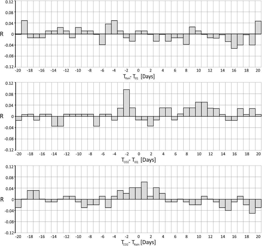
FIGURE 4. Matthews correlation coefficients in the range Δt from −20 to +20 days of the time difference between earthquake and rain events (top), ${CO}_2$ anomalies and earthquake events (middle), and ${CO}_2$ anomalies and rain events (down).

The correlation plots were drawn for time differences $∆t$ of $\pm 20$ days (i.e., $∆t=+20days$ and $∆t=-20days$ indicate an advance and a delay of 20 days, respectively, of the first type of event with respect to the second one). The correlation between rain and earthquake events is shown in Figure 4 (top diagram). We did not observe any significant correlation between meteorological and seismic phenomena. The middle plot of Figure 4 reports a significant peak of correlation between seismic and ${CO}_2$ events associated with a time difference $∆t$ of −2 days. Being $∆t$ the time difference $T_{{CO}_2}-T_{EQ}$, this is equivalent to say that on a statistical basis ${CO}_2$ anomalies tend to anticipate seismic events by 2 days. The cross-correlation peak corresponding to −2 days is 0.0947. We evaluated the uncertainty of the procedure by repeating the correlation calculus for 100 additional randomly generated earthquakes datasets. By obtaining correlation histograms with correlation peaks greater than 0.1 in only three cases (equivalent to 3%), we can discard the hypothesis that the correlation peak is due to chance. In an entirely equivalent way, by applying the Statistica^® software (Statsoft Inc., 2013), we also obtained a p-value <5%, which further confirms that the null hypothesis can be discarded. Noteworthy, the statistical procedure has highlighted the same cross-correlation peak corresponding to −2 days also when we considered a larger temporal interval ($∆t$ lag) of ±30 days, or a smaller earthquake dataset devoid of $M_L<2$ seismic events, as shown in the Supplementary Material S1.

Based on Eq. 4, the correlation peak defines the conditional probability that a seismic event may occur 2 days after a ${CO}_2$ anomaly $P\left(EQ|EC\right)$. This probability can be significantly greater than the normal frequency of earthquakes $P\left(EQ\right)=0.0277$ of a given magnitude, within a distance of $3D$ from the Gallicano station. It was calculated that $P\left(EQ|EC\right)=3.63P\left(EQ\right)$, which corresponds to a probability gain of $G\approx 3.6$. The plot at the bottom of Figure 4 represents the correlation between rainfalls and ${CO}_2$ anomalies. Here, a mild correlation aroused for a time difference $∆t=T_{{CO}_2}-T_{Rain}=+1day$, indicating that rainfalls tend to anticipate ${CO}_2$ anomalies by 1 day.

5 Conclusion

We propose a first comprehensive statistical analysis of ${CO}_2$ time series registered at the Gallicano test site, Italy, where a continuous automatic station is operating since 2003 to investigate the geochemical response to local seismic activity of a deep aquifer feeding a thermomineral spring. The availability of continuous time series emerged as an essential prerequisite to evolve towards the calculus of the conditional property of the seismic events. The focus is on ${CO}_2$ concentration values measured in spring water during the period April 2017 to April 2021. We modeled the irregular component of the ${CO}_2$ time series by a suitable fit based on the Pearson type VII distribution, and we used the Gauss’s hypergeometric function to retrieve the cumulate probability. Based on this value, we defined the threshold for 99% probability of fluctuations not occurring by chance. We calculated the cross-correlation between the binary series of ${CO}_2$ anomalies and low to moderate magnitude seismic events, disclosing a positive correlation for ${CO}_2$ anomalies occurring 2 days before the earthquakes. We extended the procedure to rainfalls vs. earthquakes, and ${CO}_2$ vs. rainfalls time series. In both cases, we estimated negligible correlations, compared to the ${CO}_2$ vs. earthquakes case. In particular, rainfall and earthquakes appeared completely uncorrelated, and just a mild correlation was observed for rains occurring 1 day before ${CO}_2$ anomalies.

A key aspect of this analysis is that the observed positive correlation between ${CO}_2$ anomalies and seismic events concerned small earthquakes with hypocenters within relevant distances from the Gallicano spring, and that this assessment is independent from the mechanisms possibly suggested to explain the cause-effect relationship between ${CO}_2$ anomalies and small seismic events. This allows us to advance the hypothesis that ${CO}_2$ variations registered in Gallicano spring water can be considered a “short-term candidate precursor” (Molchanov and Hayakawa, 2008) for low seismic activity, regardless of whether the natural mechanisms behind this correlation inherently remain poorly constrained. From this perspective, we calculated a conditional probability based on the observation of a ${CO}_2$ anomaly, which resulted in 3.6 times the unconditioned earthquake probability. The knowledge of the conditional probability of the seismic events is, in perspective, a fundamental step to switch from the mere recognition of anomalous signals to the possible forecasting of seismic events. Future work will focus on the analysis of longer time series that also includes moderate to strong seismic activity, to augment the applicability of the method in terms of seismic hazard mitigation. Moreover, it is expected that the statistical analysis of the correlation between ${CO}_2$ anomalies and seismic events can be further refined through a more in-depth examination of the possible relations between ${CO}_2$ anomalies and rainfalls.

Data availability statement

The raw data supporting the conclusion of this article will be made available by the authors, without undue reservation.

Author contributions

CF: Conceptualization, statistical method and interpretation, Writing the original draft, review and editing FG: conceptualization, hydrogeological and geochemical framework, writing the original draft, review and editing GF: instrument implementation and maintenance, acquisition of data series, writing the original draft, review and editing LP: conceptualization, hydrogeological and geochemical framework, writing the original draft, review and editing. All authors contributed to the article and approved the submitted version.

Acknowledgments

We warmly acknowledge the reviewers for their constructive criticisms, and L. Pinti for his editorial supervision.

Conflict of interest

The authors declare that the research was conducted in the absence of any commercial or financial relationships that could be construed as a potential conflict of interest.

Publisher’s note

All claims expressed in this article are solely those of the authors and do not necessarily represent those of their affiliated organizations, or those of the publisher, the editors and the reviewers. Any product that may be evaluated in this article, or claim that may be made by its manufacturer, is not guaranteed or endorsed by the publisher.

Supplementary material

The Supplementary Material for this article can be found online at: https://www.frontiersin.org/articles/10.3389/feart.2023.1128949/full#supplementary-material

References

Anderson, R. V. V. (1927). Tertiary stratigraphy and orogeny of the Northern Punjab. Geol. Soc. Am. Bull. 38, 665–720. doi:10.1130/gsab-38-665

CrossRef Full Text | Google Scholar

Barberio, M. D., Gori, F., Barbieri, M., Billi, A., Caracausi, A., De Luca, G., et al. (2020). New observations in Central Italy of groundwater responses to the worldwide seismicity. Sci. Rep. 10, 17850. doi:10.1038/s41598-020-74991-0

PubMed Abstract | CrossRef Full Text | Google Scholar

Barnes, I., Irwin, P. W., and White, D. E. (1978). “Global distribution of carbon dioxide discharges, and major zones of seismicity,” in Water resources investigation WRI 78-39 Editors I. Barnes, W. P. Irwin, and D. E. White (Washington: U.S. Geological Survey), 1–17.

Google Scholar

Bowman, D. D., Ouillon, G., Sammis, C. G., Sornette, A., and Sornette, D. (1998). An observational test of the critical earthquake concept. J. Geophys. Res. 103, 24359–24372. doi:10.1029/98JB00792

CrossRef Full Text | Google Scholar

Box, G. E. P., and Jenkins, G. M. (1976). Time series analysis: Forecasting and control. San Francisco: Holden Day.

Google Scholar

Bräuer, K., Kämpf, H., Strauch, G., and Weise, S. M. (2003). Isotopic evidence (³He/⁴He, δ¹³C-CO₂) of fluid-triggered intraplate seismicity. J. Geophys. Res. 108 (B2), 2070. doi:10.1029/2002JB002077

CrossRef Full Text | Google Scholar

Brodsky, E. E., Roeloffs, E., Woodcock, D., Gall, I., and Manga, M. (2003). A mechanism for sustained groundwater pressure changes induced by distant earthquakes. J. Geophys. Res. 108, 88. doi:10.1029/2002JB002321

CrossRef Full Text | Google Scholar

Camarda, M., Caracausi, A., Chiaraluce, L., De Gregorio, S., and Favara, R., (2018). Two years of geochemical monitoring along the Alto Tiberina Fault (Italy): New inferences on fluids and seismicity in central Apennines. In Proceedings of the 20th EGU General Assembly, Vienna, Austria, 4–13 April 2018.

Google Scholar

Camarda, M., De Gregorio, S., Di Martino, R. M. R., and Favara, R. (2016). Temporal and spatial correlations between soil CO₂ flux and crustal stress. J. Geophys. Res. 121, 7071–7085. doi:10.1002/2016JB013297

CrossRef Full Text | Google Scholar

Cardellini, C., Chiodini, G., Frondini, F., Avino, R., Bagnato, E., Caliro, S., et al. (2017). Monitoring diffuse volcanic degassing during volcanic unrests: The case of campi flegrei (Italy). Sci. Rep. 7 (1), 6757–6815. doi:10.1038/s41598-017-06941-2

PubMed Abstract | CrossRef Full Text | Google Scholar

Chiodini, G., Cardellini, C., Amato, A., Boschi, E., Caliro, S., Frondini, F., et al. (2004). Carbon dioxide Earth degassing and seismogenesis in central and southern Italy. Geophys. Res. Lett. 31 (7). doi:10.1029/2004GL019480

CrossRef Full Text | Google Scholar

Chiodini, G., Cardellini, C., Di Luccio, F., Selva, J., Frondini, F., Caliro, S., et al. (2020). Correlation between tectonic CO₂ Earth degassing and seismicity is revealed by a 10-year record in the Apennines, Italy. Sci. Adv. 6 (35), eabc2938. eabc 2938. doi:10.1126/sciadv.abc2938

PubMed Abstract | CrossRef Full Text | Google Scholar

Cioni, R., Guidi, M., Pierotti, L., and Scozzari, A. (2007). An automatic monitoring network installed in Tuscany (Italy) for studying possible geochemical precursory phenomena. Nat. Hazards Earth Syst. Sci. 7, 405–416. doi:10.5194/nhess-7-405-2007

CrossRef Full Text | Google Scholar

Cooper, H. H., Bredehoeft, J. D., Papadopulos, I. S., and Bennett, R. R. (1965). The response of well-aquifer systems to seismic waves. J. Geophys. Res. 70, 3915–3926. doi:10.1029/JZ070i016p03915

CrossRef Full Text | Google Scholar

Dall'Aglio, M., Quattrocchi, F., and Venanzi, G. (1990). La stazione automatica per lo studio dei precursori geochimici nei colli albani: Il prototipo del sottosistema geochimico della rete sismica nazionale dell'ING. Proc. IX Convegno GNGTS 1990, CNR-Roma 1990, 95–100. (in Italian).

Google Scholar

Di Bello, G., Heinicke, J., Koch, U., Lapenna, V., Macchiato, M., Martinelli, G., et al. (1998). Geophysical and geochemical parameters jointly monitored in a seismic area of Southern Apennines (Italy). Phys. Chem. Earth 23, 909–914. doi:10.1016/S0079-1946(98)00118-9

CrossRef Full Text | Google Scholar

Di Martino, R. M., Camarda, M., Gurrieri, S., and Valenza, M. (2013). Continuous monitoring of hydrogen and carbon dioxide at Mt Etna. Chem. Geol. 357, 41–51. doi:10.1016/j.chemgeo.2013.08.023

CrossRef Full Text | Google Scholar

DISS Working Group (2021). Database of individual seismogenic sources (DISS), version 3.3.0: A compilation of potential sources for earthquakes larger than M 5.5 in Italy and surrounding areas. United States: Istituto Nazionale di Geofisica e Vulcanologia. doi:10.13127/diss3.3.0

CrossRef Full Text | Google Scholar

Dobrovolsky, I. P., Zubkov, S. I., and Miachkin, V. I. (1979). Estimation of the size of earthquake preparation zones. Pure Appl. Geophys. Pageoph 117, 1025–1044. doi:10.1007/bf00876083

CrossRef Full Text | Google Scholar

Fidani, C. (2018). Improving earthquake forecasting by correlations between strong earthquakes and NOAA electron bursts. Terr. Atmos. Ocean. Sci. 29 (2), 117–130. doi:10.3319/tao.2017.10.06.01

CrossRef Full Text | Google Scholar

Fidani, C. (2020). Probability, causality and false alarms using correlations between strong earthquakes and NOAA high energy electron bursts. Ann. Geophys. 63 (5), 543. doi:10.4401/ag-7957

CrossRef Full Text | Google Scholar

Fidani, C. (2021). West pacific earthquake forecasting using NOAA electron bursts with independent L-shells and ground-based magnetic correlations. Front. Earth Sci. 9, 673105. doi:10.3389/feart.2021.673105

CrossRef Full Text | Google Scholar

Fischer, T., Matyska, C., and Heinicke, J. (2017). Earthquake-enhanced permeability – evidence from carbon dioxide release following the ML 3.5 earthquake in West Bohemia. Earth Planet. Sci. Lett. 460, 60–67. doi:10.1016/j.epsl.2016.12.001

CrossRef Full Text | Google Scholar

Gardner, J. K., and Knopoff, L. (1974). Is the sequence of earthquakes in Southern California, with aftershocks removed, Poissonian? Bull. Seismol. Soc. Am. 64, 1363–1367. doi:10.1785/bssa0640051363

CrossRef Full Text | Google Scholar

Gherardi, F., and Pierotti, L. (2018). The suitability of the Pieve Fosciana hydrothermal system (Italy) as a detection site for geochemical seismic precursors. Appl. Geochem. 92, 166–179. doi:10.1016/j.apgeochem.2018.03.009

CrossRef Full Text | Google Scholar

Giudicepietro, F., Chiodini, G., Caliro, S., De Cesare, W., Esposito, A. M., Galluzzo, D., et al. (2019). Insight into Campi Flegrei caldera unrest through seismic tremor measurements at Pisciarelli fumarolic field. Geochem. Geophys. Geosystems 20 (11), 5544–5555. doi:10.1029/2019gc008610

CrossRef Full Text | Google Scholar

Gold, T., and Soter, S. (1979). Brontides: Natural explosive noises. Science 204, 371–375. doi:10.1126/science.204.4391.371

PubMed Abstract | CrossRef Full Text | Google Scholar

Gold, T., and Soter, S. (1985). Fluid ascent through the solid lithosphere and its relation to earthquakes. Pure Appl. Geophys. 122 (2), 492–530. doi:10.1007/bf00874614

CrossRef Full Text | Google Scholar

Gold, T., and Soter, S. (1981). Response: Natural explosive noises. Science 212, 1297–1298. doi:10.1126/science.212.4500.1297

PubMed Abstract | CrossRef Full Text | Google Scholar

Gold, T. (1979). Terrestrial sources of carbon and earthquake outgassing. J. Petroleum Geol. 1 (3), 3–19. doi:10.1111/j.1747-5457.1979.tb00616.x

CrossRef Full Text | Google Scholar

Gold, T. (1999). The deep hot biosphere. New York: Springer, 235.

Google Scholar

He, A., and Singh, R. P. (2020). Coseismic groundwater temperature response associated with the Wenchuan earthquake. Pure Appl. Geophys. 177, 109–120. doi:10.1007/s00024-019-02097-4

CrossRef Full Text | Google Scholar

Heinicke, J., Koch, U., and Martinelli, G. (1995). CO₂ and Radon measurements in the Vogtland area (Germany) - a contribute to earthquake prediction research. Geoph. Res. Lett. 22 (7), 771–774. doi:10.1029/94gl03074

CrossRef Full Text | Google Scholar

Heinicke, J., Martinelli, G., and Telesca, L. (2012). Geodynamically induced variations in the emission of CO₂ gas at san faustino (central Apennines, Italy). Geofluids 12, 123–132. doi:10.1111/j.1468-8123.2011.00345.x

CrossRef Full Text | Google Scholar

Hubbert, M. K., and Rubey, W. W. (1959). Role of fluid pressure in mechanics of overthrust faulting: I. Mechanics of fluid-filled porous solids and its application to overthrust faulting. GSA Bull. 70 (2), 115–166.

CrossRef Full Text | Google Scholar

Hunt, J. A., Zafu, A., Mather, T. A., Pyle, D. M., and Barry, P. H. (2017). Spatially variable CO₂ degassing in the main Ethiopian rift: Implications for magma storage, volatile transport, and rift-related emissions. Geochem. Geophys. Geosyst. 18, 3714–3737. doi:10.1002/2017gc006975

CrossRef Full Text | Google Scholar

Irwin, W. P., and Barnes, I. (1980). Tectonic relations of carbon dioxide discharges and earthquakes. J. Geophys. Res. 85 (B6), 3115–3121. doi:10.1029/jb085ib06p03115

CrossRef Full Text | Google Scholar

Italiano, F., Martelli, M., Martinelli, G., Nuccio, P. M., and Paternoster, M. (2001). Significance of earthquake-related anomalies in fluids of Val D’Agri (southern Italy). Terra nova. 13 (4), 249–257. doi:10.1046/j.1365-3121.2001.00346.x

CrossRef Full Text | Google Scholar

Italiano, F., Martinelli, G., and Rizzo, A. (2004). Geochemical evidence of seismogenic-induced anomalies in the dissolved gases of thermal waters: A case study of umbria (central Apennines, Italy) both during and after the 1997–1998 seismic swarm. Geochem. Geophys. Geosystems 5 (11), Q11001. doi:10.1029/2004GC000720

CrossRef Full Text | Google Scholar

Johnson, N. L., Kotz, S., and Balakrishnan, N. (1995). “Chapter 28,” in Continuous univariate distributions. 2nd ed. (United States: Wiley).

Google Scholar

King, C. Y., Zhang, W., and Zhang, Z. (2006). Earthquake-induced groundwater and gas changes. Pure Appl. Geophys. 163 (4), 633–645. doi:10.1007/s00024-006-0049-7

CrossRef Full Text | Google Scholar

Kingsley, , Biagi, P., Piccolo, R., Capozzi, V., Ermini, A., Khatkevich, Y., et al. (2001). Hydrogeochemical precursors of strong earthquakes: A realistic possibility in kamchatka. Phys. Chem. Earth C 26 (10-12), 769–774. doi:10.1016/s1464-1917(01)95023-8

CrossRef Full Text | Google Scholar

Lee, H., Muirhead, J. D., Fischer, T. P., Ebinger, C. J., Kattenhorn, S. A., Sharp, Z. D., et al. (2016). Massive and prolonged deep carbon emissions associated with continental rifting. Nat. Geosci. 9, 145–149. doi:10.1038/ngeo2622

CrossRef Full Text | Google Scholar

Makridakis, S., Wheelwright, S. C., and Hyndman, R. J. (1998). Forecasting methods and applications. 3rd ed. New York: John Wiley and Sons, 642.

Google Scholar

Manga, M., and Wang, C. Y. (2015). Earthquake hydrology. Treatise Geophys. 2015, 305–328. doi:10.1016/b978-0-444-53802-4.00082-8

CrossRef Full Text | Google Scholar

Martinelli, G., and Albarello, D. (1997). Main constraints for siting monitoring networks devoted to the study of earthquake related phenomena in Italy. Ann. Geophys. 40, 1505–1522.

Google Scholar

Martinelli, G., Ciolini, R., Facca, G., Fazio, F., Gherardi, F., Heinicke, J., et al. (2021). Tectonic-related geochemical and hydrological anomalies in Italy during the last fifty years. Minerals 11, 107. doi:10.3390/min11020107

CrossRef Full Text | Google Scholar

Martinelli, G., and Dadomo, A. (2017). Factors constraining the geographic distribution of earthquake geochemical and fluid-related precursors. Chem. Geol. 469, 176–184. doi:10.1016/j.chemgeo.2017.01.006

CrossRef Full Text | Google Scholar

Martinelli, G., Facca, G., Genzano, N., Gherardi, F., Lisi, M., Pierotti, L., et al. (2020). Earthquake-related signals in Central Italy detected by hydrogeochemical and satellite techniques. Front. Earth Sci. 8, 584716. doi:10.3389/feart.2020.584716

CrossRef Full Text | Google Scholar

Massin, F., Farrell, J., and Smith, R. B. (2013). Repeating earthquakes in the yellowstone volcanic field: Implications for rupture dynamics, ground deformation, and migration in earthquake swarms. J. Volcanol. Geotherm. Res. 257, 159–173. doi:10.1016/j.jvolgeores.2013.03.022

CrossRef Full Text | Google Scholar

Matthews, B. W. (1975). Comparison of the predicted and observed secondary structure of T4 phage lysozyme. Biochimica Biophysica Acta (BBA) - Protein Struct. 405 (2), 442–451. doi:10.1016/0005-2795(75)90109-9

CrossRef Full Text | Google Scholar

Miller, S. A. (2013). Advances in Geophysics, R. Dmowska, Ed. (Amsterdam: Elsevier). 1–46.

Google Scholar

Molchanov, O. A., and Hayakawa, M. (2008). Seismo-electromagnetics and related phenomena. Tokyo: Terrapub.

Google Scholar

Molli, G., Manighetti, I., Bennett, R., Malavieille, J., Serpelloni, E., Storti, F., et al. (2021). Active fault systems in the inner northwest Apennines, Italy: A reappraisal one century after the 1920 Mw∼6.5 fivizzano earthquake. Geosciences 11 (3), 139. doi:10.3390/geosciences11030139

CrossRef Full Text | Google Scholar

Netreba, A. V., Fridman, A. I., Plotnikov, I. A., and Khurin, M. I. (1971). On the large-scale mapping of closed ore-bearing areas in the north Caucasus with the uses of gas surveying as a geochemical method. Geokhimia 8, 1016–1021. (in Russian).

Google Scholar

Ohnaka, M. (1992). Earthquake source nucleation: A physical model for short term precursors. Tectonophysics 211, 149–178. doi:10.1016/0040-1951(92)90057-D

CrossRef Full Text | Google Scholar

Pearson, K. (1916). Mathematical contributions to the theory of evolution, XIX: Second supplement to a memoir on skew variation. Philosophical Trans. R. Soc. A 216 (538–548), 429–457.

Google Scholar

Pering, T. D., Tamburello, G., McGonigle, A. J. S., Aiuppa, A., Cannata, A., Giudice, G., et al. (2014). High time resolution fluctuations in volcanic carbon dioxide degassing from Mount Etna. J. Volcanol. Geotherm. Res. 270, 115–121. doi:10.1016/j.jvolgeores.2013.11.014

CrossRef Full Text | Google Scholar

Pierotti, L., Botti, F., D’Intinosante, V., Facca, G., and Gherardi, F. (2015). Anomalous CO₂ content in the Gallicano thermo-mineral spring (serchio valley, Italy) before the 21 june 2013, alpi apuane earthquake (M= 5.2). Phys. Chem. Earth, Parts A/B/C 85, 131–140. doi:10.1016/j.pce.2015.02.007

CrossRef Full Text | Google Scholar

Pierotti, L., Gherardi, F., Facca, G., Piccardi, L., and Moratti, G. (2017). Detecting CO₂ anomalies in a spring on Mt. Amiata volcano (Italy). Phys. Chem. Earth, Parts A/B/C 98, 161–172. doi:10.1016/j.pce.2017.01.008

CrossRef Full Text | Google Scholar

Reasenberg, P. (1985). Second-order moment of central California seismicity, 1969-1982. J. Geophys. Res. 90, 5479–5495. doi:10.1029/jb090ib07p05479

CrossRef Full Text | Google Scholar

Rebetsky, Y. L., and Lermontova, A. S. (2018). On the long-range influence of earthquake rupture zones. J. Volcanol. Seismol. 12, 341–352. doi:10.1134/S0742046318050068

CrossRef Full Text | Google Scholar

Rikitake, T. (1994). Nature of macro-anomaly precursory to an earthquake. J. Phys. Earth 42, 149–163. doi:10.4294/jpe1952.42.149

CrossRef Full Text | Google Scholar

Rovida, A., Locati, M., Camassi, R., Lolli, B., Gasperini, P., and Antonucci, A. (2022). Catalogo Parametrico dei Terremoti Italiani (CPTI15). versione 4.0. Italy: Istituto Nazionale di Geofisica e Vulcanologia. doi:10.13127/CPTI/CPTI15.4

CrossRef Full Text | Google Scholar

Shi, Z., and Wang, G. (2014). Hydrological response to multiple large distant earthquakes in the Mile well, China. J. Geophys. Res. 119, 2448–2459. doi:10.1002/2014JF003184

CrossRef Full Text | Google Scholar

Sil, S., and Freymueller, J. T. (2006). Well water level changes in Fairbanks, Alaska, due to the great Sumatra-Andaman earthquake. Earth Planets Space 58, 181–184. doi:10.1186/BF03353376

CrossRef Full Text | Google Scholar

Statsoft Inc. (2013). STATISTICA (data analysis software system) version 12 for windows: Statistics. Tulsa, OK.: STATSOFT Inc.

Google Scholar

Stucchi, M., Meletti, C., Montaldo, V., Crowley, H., Calvi, G. M., and Boschi, E. (2011). Seismic hazard assessment (2003–2009) for the Italian building code. Bull. Seismol. Soc. Am. 101 (4), 1885–1911. doi:10.1785/0120100130

CrossRef Full Text | Google Scholar

Tamburello, G., Pondrelli, S., Chiodini, G., and Rouwet, D. (2018). Global-scale control of extensional tectonics on CO₂ Earth degassing. Nat. Commun. 9, 4608. doi:10.1038/s41467-018-07087-z

PubMed Abstract | CrossRef Full Text | Google Scholar

Velleman, P. F., and Hoaglin, D. C. (1981). Applications, basics, and computing of exploratory data analysis. Boston, MA: Duxbury Press.

Google Scholar

Ventura, G., Cinti, F. R., Di Luccio, F., and Pino, N. A. (2007). Mantle wedge dynamics versus crustal seismicity in the Apennines (Italy). Geochem. Geophys. Geosys. 8, Q02013. doi:10.1029/2006gc001421

CrossRef Full Text | Google Scholar

Weinlich, F. H., Faber, E., Boušková, A., Horálek, J., Teschner, M., and Poggenburg, J. (2006). Seismically induced variations in mariánské lázně fault gas composition in the NW bohemian swarm quake region, Czech republic—a continuous gas monitoring. Tectonophysics 421 (1-2), 89–110. doi:10.1016/j.tecto.2006.04.012

CrossRef Full Text | Google Scholar

Wiemer, S. (2001). A software package to analyze seismicity: ZMAP. Seismol. Res. Lett. 72 (3), 373–382. doi:10.1785/gssrl.72.3.373

CrossRef Full Text | Google Scholar

Woith, H., Petersen, G. M., Hainzl, S., and Dahm, T. (2018). Review: Can animals predict earthquakes? Bull. Seismol. Soc. Am. 108, 1031–1045. doi:10.1785/0120170313

CrossRef Full Text | Google Scholar

Yoshida, K., and Hasegawa, A. (2018). Hypocenter migration and seismicity pattern change in the yamagata-fukushima border, NE Japan, caused by fluid movement and pore pressure variation. J. Geophys. Res. Solid Earth 123 (6), 5000–5017. doi:10.1029/2018jb015468

CrossRef Full Text | Google Scholar

Zhang, Y., Fu, L. Y., Huang, F., and Chen, X. (2015). Coseismic water-level changes in a well induced by teleseismic waves from three large earthquakes. Tectonophysics 651, 232–241. doi:10.1016/j.tecto.2015.02.027

CrossRef Full Text | Google Scholar