Crosstalk attenuation for imaging of multiples based on angle gather residual moveout analysis

Imaging of multiples, as a supplement to imaging of primaries, can provide a wider range of subsurface illumination. Therefore, it can provide more detailed information on subsurface structures. However, imaging of multiples suffers from crosstalk issues generated by unrelated events. Many strategies have been proposed to attenuate crosstalk, among which the angle domain Radon crosstalk attenuation algorithm achieves good application effect. In the angle domain, the true imaging is flat, while the crosstalk events have moveouts. Therefore, it is convenient to identify the crosstalk in angle gathers using the Radon transform. However, the conventional Radon transform lacks a quantitative description for crosstalk in angle gathers, which would affect the accuracy of crosstalk attenuation. In this paper, residual moveout kernels are derived with a Radon transform to attenuate crosstalk in angle gathers for imaging of multiples. First, two types of residual moveout (RMO) equations are derived based on the causality of crosstalk. A three-layer model is used to verify the correctness of the analytical solutions. Then, based on the derived equations, the two types of crosstalk can be attenuated respectively in the Radon domain. Synthetic experiments demonstrate that the derived RMO equations can effectively attenuate the crosstalk events in imaging of multiples.

1 Introduction

Unlike the conventional approach treats surface-related multiples as noises, imaging of multiples uses them as effective signals to image subsurface structures. Since the multiples have more propagation paths, imaging of multiples can provide more detailed information on subsurface structures (Berkhout and Verschuur, 2003). There are three main approaches for implementing imaging of multiples (Lu et al., 2021). The up-down wavefield imaging method (Berkhout and Verschuur, 1994; Liu et al., 2011) replaced the source wavelet with primary and multiples and used multiples as receivers for migration. The seismic interferometry proposed by Schuster and Rickett (2000) transformed multiples into primary and imaged them. In addition, the Marchenko imaging proposed by Wapenaar et al. (2014) used surface-related multiples and internal multiples for migration (Singh et al., 2017; Gu and Wu, 2022).

Although imaging of multiples has been implemented through different approaches, there still remains many undesired crosstalk issues in imaging result. Crosstalk is generated due to the correlation of unrelated events (Liu et al., 2016; Lu et al., 2016; Lu et al., 2021). These crosstalk issues introduce difficulties in the interpretation of the imaging results. Therefore, it is crucial to attenuate them. Many methods have been proposed to attenuate crosstalk for imaging of multiples. One category is to remove crosstalk during the migration, such as the least-squares migration (LSM) (Berkhout, 2014; Ordoñez et al., 2014; Zhang and Schuster, 2014; Tu and Herrmann, 2015; Wong et al., 2015; Lu et al., 2018; Lu et al., 2021) and imaging using controlled-order multiples (Liu et al., 2016). However, such methods usually require a huge amount of computation or complete separation of different orders multiples. The other category is to deal with the crosstalk after migration, such as the angle domain Radon crosstalk suppression (Wang et al., 2014; Wong et al., 2015). In the angle domain, the moveouts of imaging are flat when imaging of multiples using the correct velocity, whereas the moveouts of crosstalk are curved. The Radon transform can attenuate curved events in angle gathers, and then the crosstalk issues can be addressed without increasing the calculation cost and separation of different orders multiples. However, this strategy using the tangent-squared approximation as the kernel function of the Radon transform lacks a quantitative explanation of the theoretical mechanism of crosstalk and therefore affects the accuracy of crosstalk attenuation.

To enhance the effectiveness of the Radon transform to attenuate the crosstalk in angle gathers, a better understanding of the crosstalk generation mechanism is needed. Mathematically, the crosstalk in angle gathers can be calculated and attenuated based on the causality (Lu et al., 2016; Lu et al., 2021). Here, we propose a method to attenuate crosstalk by applying the residual moveouts of crosstalk as kernel functions in the Radon transform. Imaging results with an improved signal-to-noise ratio can then be produced.

In this paper, for the purpose of convenience in analyzing the residual moveouts for crosstalk, we first review the principle of classifying crosstalk according to the causality. Next, we derive the RMO equations for two types of crosstalk in angle gathers based on the classification principle and verify the correctness of the equations in angle gathers using a three-layer model. Then, we compare the derived RMO equations with the tangent square approximation equation as kernel functions for the Radon transform and demonstrate the effectiveness of our method. Finally, we perform a numerical experiment with a subset of the Sigsbee2b model, which proves that our proposed method can attenuate most of the crosstalk and improve the signal-to-noise ratio of the imaging results.

2 Methodology

2.1 The classification of crosstalk

In this section, we explain the generation and classification of crosstalk in the imaging of multiples. We assume that the sea surface is a fully reflective interface. Therefore, in the imaging of multiples, the free-surface seismic data are multiplied by −1, loaded at the sea surface, and propagated forward as virtual sources to composite the subsurface source wavefields. Then, the images using cross-correlation imaging conditions in the frequency domain can be computed as:

$I_m\left(\mathbf{x}\right)={\displaystyle \sum }_{\omega }\left[{\displaystyle \sum }_j{S}_j\left(\mathbf{x};\omega \right){\displaystyle \sum }_l{R}_l\left(\mathbf{x};\omega \right)\right](1)$

where I_m represents the imaging results of multiples; x represents the vector coordinates of the imaging point; ω is the frequency; S_j and R_l respectively represent the forward-propagated source wavefields and the backward-propagated receiver wavefields; j and l respectively represent primary and the order of multiples for the source wavefields and receiver wavefields. When j equals 1, $S_j$ represents the forward-propagated source wavefield of the primaries, and when j equals n (n≠1), $S_j$ represents the forward-propagated source wavefield of the (n-1) thorder multiples. Similarly, when l equals 1, $R_l$ represents the backward-propagated source wavefield of the primaries, and when l equals n, $R_l$ represent the backward-propagated source wavefield of the (n-1) th-order multiples.

Eq 1 donates not only the correct imaging results of multiples, but also the crosstalk. To have a more intuitive understanding of the formation for crosstalk, we rewrite Eq 1 as:

$\begin{array}{l}{I}_m\left(\mathrm{x}\right)={\displaystyle \sum }_{\omega }\left[S_1\left(\mathrm{x};\omega \right)R_2\left(\mathrm{x};\omega \right)+S_2\left(\mathrm{x};\omega \right)R_3\left(\mathrm{x};\omega \right)+S_3\left(\mathrm{x};\omega \right)R_4\left(\mathrm{x};\omega \right)+\cdots \right]\\ +{\displaystyle \sum }_{\omega }\left[S_1\left(\mathrm{x};\omega \right)R_3\left(\mathrm{x};\omega \right)+S_2\left(\mathrm{x};\omega \right)R_4\left(\mathrm{x};\omega \right)+S_3\left(\mathrm{x};\omega \right)R_5\left(\mathrm{x};\omega \right)+\cdots \right],\\ +{\displaystyle \sum }_{\omega }\left[S_1\left(\mathrm{x};\omega \right)R_1\left(\mathrm{x};\omega \right)+S_2\left(\mathrm{x};\omega \right)R_1\left(\mathrm{x};\omega \right)+S_2\left(\mathrm{x};\omega \right)R_2\left(\mathrm{x};\omega \right)+...\right]\end{array}(2)$

In Eq 2, the images can be divided into three parts. The first part corresponds to the correct imaging results of multiples, for example, $S_1$ and $R_2$ constitute effective imaging according to the ray travel time and the cross-correlation imaging conditions (Clarebout, 1978). The second part and the third part are corresponding to the crosstalk generated by uncorrelated events. (Lu et al., 2021). classify the above crosstalk into two types based on causality, which are causal crosstalk and anti-causal crosstalk. To better understand the generation formation of crosstalk, we display the ray path diagrams for the two types of crosstalk (Figure 1).

FIGURE 1

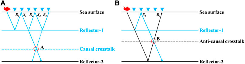
FIGURE 1. The ray paths diagrams for the two types of crosstalk. (A) The diagram of trajectories for causal crosstalk, (B) the diagram of trajectories for anti-causal crosstalk. In (A), The virtual source S₁ (recorded primary reflections carried with information of reflector-1 as the source wavefield) and receiver wavefield R₃ (second order multiple) can generate causal crosstalk at position (A). In (B), the virtual source S₁ and receiver wavefield R₃ (recorded primary reflections carried with information of reflector-2 as the receiver wavefield) can generate anti-causal crosstalk at position (B).

We illustrate the diagram of trajectories for two types of crosstalk based on the cross-correlation imaging conditions from the second part and the third part in Eq 2 (Figure 1). In Figure 1A, the recorded primary reflection carried with information of reflector-1 at the sea surface forward propagated as the source wavefield $S_1$ (dashed blue arrow), and it cross-correlates with the receiver wavefield $R_3$ backward propagated (dashed blue arrow), which generates the crosstalk at position A. These crosstalk events are related to the wavefields after reflection with the reflector-1 and are deeper than the actual depth of reflector-1. Therefore, these events are called “causal crosstalk”. Similarly, in Figure 1B, the recorded primary reflection carried with information of reflector-2 backward propagated as the source wavefield $R_1$ (black arrow), and it interacts with the virtual source $S_1$ (dashed blue arrow), which generates the crosstalk at location B. These events carried the information of reflector-2 are shallower than the real location, and actually contrary to the actual causality. Therefore, they are called “anti-causal crosstalk” (Lu et al., 2021).

The two types of crosstalk events are easily identified in simple models by their causality. However, the propagation paths of the wavefields are hard to judge and identify when there are many subsurface reflectors and complex structures. With the understanding of the classification mechanism of crosstalk, we can calculate the residual moveouts of the two types of crosstalk independently in angle gathers. And then, based on the derived equations, we can address the crosstalk issues under complex scenarios.

2.2 The calculation for the residual moveouts of crosstalk in the angle domain

Due to the arrival-time differences, the imaging events and crosstalk components have different moveouts in the angle domain. Based on the differences in moveouts, we can attenuate crosstalk in angle gathers using the Radon transform. To quantitatively characterize the moveouts in the angle domain for crosstalk and attenuate them, in this section, we first derive the residual moveout equations for two types of crosstalk.

There are many methods for generating angle gathers, such as subsurface offset-to-angle conversion (Sava and Fomel, 2003; Biondi and Symes, 2004) and directional vector (Yoon and Marfurt, 2006; Xu et al., 2011). In this paper, we use the subsurface offset-to-angle algorithm to calculate the imaging angles. Based on the slant stack principle proposed by Sava and Fomel (2003), the subsurface offset gathers generated after the migration can be converted into angle gathers. The subsurface offset-angle conversion can be expressed as:

$\tan \gamma =-\frac{\partial z}{\partial h}{|}_{t,x}.(3)$

In Eq 3, t is the travel time, z and x are the depth and vertical position of the reflection point, respectively, and h is the local subsurface half-offset after downward continuation (Figure 2). The crosstalk events can be converted from the subsurface offset domain to the angle domain based on Eq 3. Meanwhile, using this conversion approach, we can derive the RMO equations for two types of crosstalk in angle gathers.

FIGURE 2

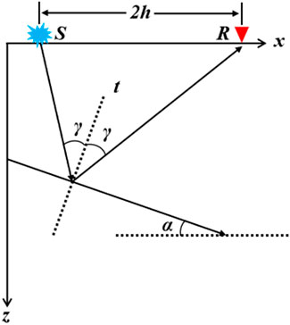
FIGURE 2. Reflection ray paths in a normal velocity medium. a is the inclination of the reflector and γ is the angle of the ray normal to the reflector. S and R are the position of the wavefield continued to the local source and receiver points in the subsurface respectively. h is the local subsurface half offset after the downward continuation. z and x are the depth and vertical position of the reflection point, respectively.

2.2.1 Calculation of the residual moveout for causal crosstalk

There are two types of crosstalk, which are causal crosstalk and anti-causal crosstalk. In this section, we derive the RMO equation for causal crosstalk. First, we can obtain the relationship between depth and subsurface offset based on the results after migration and then use the subsurface offset-to-angle conversion relationship to calculate the RMO equation for causal crosstalk.

Alvarez et al. (2007) gives the RMO equation for multiples in angle gathers for imaging of primaries. The causal crosstalk events in imaging of multiples have similar kinematic characteristics as the previous ones in angle gathers. Thus, we use the approach of Alvarez et al. (2007) to obtain the RMO equation for causal crosstalk.

In Figure 3, based on the travel time and the trigonometric relationship, the forward-propagated virtual source wavefield S₁ ends up at a specific location (x_Is, z_I) in the subsurface (as purple dashed circles indicate) after migration. Similarly, the backward-propagated receiver wavefield R₃ ends up at (x_Ir, z_I). The causal crosstalk can be generated by cross-correlating the source and receiver wavefield propagated into the subsurface. Combining the above principles and the derivation of Alvarez et al. (2007), the depth z_I of the imaged causal crosstalk and the subsurface half-offset h_I can be displayed as:

$z_I=z_a+\rho \sqrt{z_a^2+\frac{h_I^2}{1-{\rho }^2}}\left(\rho \ne 1\right),(4)$

where ρ is equal to V₂/V₁; V₁ and V₂ are the velocity of the first and second layers, respectively; z_a is the depth of the reflector-1.

FIGURE 3

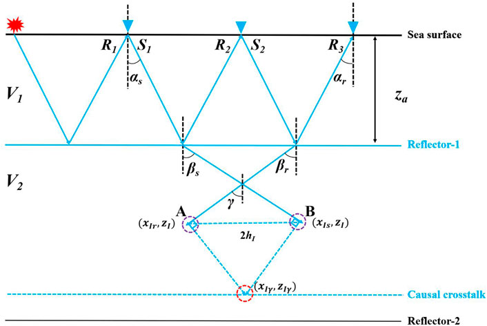
FIGURE 3. Ray paths for generating causal crosstalk. V₁ and V₂ are the velocity of the first and second layers, respectively. z_a is the depth of the reflector-1. α_s and α_r are the incident and emergent angles of the source and receiver rays with respect to the vertical direction. β_s and β_r are the angles of the source and the receiver rays with respect to the vertical direction after refraction by the reflector-1. γ is the half-aperture angle, which is equal to (β_s+β_r)/2.

Based on Eqs 3, 4, we can obtain the relationship between the depth z_Iγ and the half-aperture angle γ in the angle domain as:

$z_{I\gamma }={\mathrm{z}}_a\left\{1+\frac{\cos \gamma \left[{\rho }^2-\tan {}^2\gamma \left(1-{\rho }^2\right)\right]}{\sqrt{{\rho }^2-\sin {}^2\gamma }}\right\}.(5)$

Eq. 5 is the moveout equation for causal crosstalk in angle gathers. In Eq. 5, when reflector-2 has the same velocity as reflector-1 (ρ=1), the imaging depth for causal crosstalk in angle gathers is z_Iγ(0)=2z_a. This indicates that when multiples are used for migration at a constant velocity, the causal crosstalk is a flat moveout in angle gathers. That is, the imaging depth does not vary with the change of angle. By subtracting the flat moveout from Eq. 4, the RMO for causal crosstalk in angle gathers can be followed as:

$\Delta n_{RMO}=z_{I\gamma }\left(0\right)-z_{I\gamma }=z_a\left\{\rho -\frac{\cos \gamma \left[{\rho }^2-\tan {}^2\gamma \left(1-{\rho }^2\right)\right]}{\sqrt{{\rho }^2-\sin {}^2\gamma }}\right\},(6)$

where z_Iγ(0) denotes the depth of causal crosstalk when the velocity of reflector-1 (ρ=1) is used for the migration. Eq. 6 shows the relationship between the RMO of the causal crosstalk in angle gathers and the half-aperture angle γ and it qualitatively characterizes the kinematics mechanisms of the causal crosstalk when the multiples are migrated with the correct velocity.

2.2.2 Calculation of the residual moveout for anti-causal crosstalk

Similar to the calculation of the RMO equation for causal crosstalk, we first obtain the relationship between imaging depth and subsurface offset for anti-causal crosstalk based on travel time and Snell’s law. Then, we calculate the RMO equation for anti-causal crosstalk in terms of the subsurface offset-to-angle conversion relationship proposed by Sava and Fomel (2003). However, when anti-causal crosstalk events are imaged, they involve information from two different reflectors and therefore have different kinematic mechanisms compared to causal crosstalk events. In the following, we give a detailed derivation of the RMO equation for anti-causal crosstalk in angle gathers.

The RMO equation for anti-causal crosstalk can actually be calculated based on the travel time of the CMP gathers and Snell’s law. In Figure 4, the forward-propagated virtual source wavefield S₁ with information of reflector-1, and the backward-propagated receiver wavefield R₃ with information of reflector-2, end up at a particular location (x_Is, z_I) and (x_Ir, z_I) in the subsurface (as purple dashed circles indicate) after migration, respectively. By correlating the two wavefields, the anti-causal crosstalk will be generated.

FIGURE 4

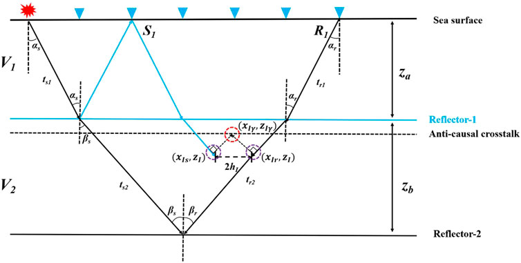
FIGURE 4. Ray paths for generating anti-causal crosstalk. V₁ and V₂ are the velocity of the first and second layers, respectively. z_a and z_b are the depth of the reflector-1 and reflector-2. α_s and α_r are the incident and emergent angles of the source and receiver rays with respect to the vertical direction. β_s and β_r are the angles of the source and the receiver rays with respect to the vertical direction after refraction by the reflector-1. γ is the half-aperture angle, which is equal to (β_s+β_r)/2. h_I is the subsurface half-offset, which is equal to (x_Ir-x_Is)/2.

Based on the cross-correlation imaging conditions, the anti-causal crosstalk follows the same travel time in imaging as the primary from the second layer. As shown in Figure 4, the total travel time in the second layer contains four main components, which can be described as:

$T=t_{s1}+t_{s2}+t_{r2}+t_{r1},(7)$

where the subscript s refers to the source-side rays and the subscript r refers to the receiver-side rays; t_s1 and t_s2 represent the time of forward-propagating rays from virtual source to reflector-1, from reflector-1 to reflector-2; t_r1 and t_r2 represent the time of backward-propagating rays from receiver side to reflector-1, from reflector-1 to reflector-2.

Based on Equation 7 and the geometry relationship shown in Figure 4, we can calculate the depth z_I of the crosstalk event and the half-offset h_I as:

$\left\{\begin{array}{l}{z}_I=z_a+z_b-V_2{t}_{s1}\cos {\beta }_s\\ h_I=\left({\rho }^2-1\right)V_1{t}_{s1}\sin {\alpha }_s\end{array}\right.,(8)$

where z_I represents the depth of the anti-causal crosstalk events.

Combining Eq 8 and the travel time relationship, the relationship between the depth z_I of causal crosstalk and the subsurface half-offset h_I can be computed as:

$z_I=z_a+z_b-\rho \sqrt{z_a^2-\frac{h_I^2}{{\rho }^2-1}}.(9)$

According to the principle of slant stack (Eq. 3), we can turn Eq 9 into the relationship between the depth of anti-causal crosstalk in angle gathers and half-aperture angle. As shown in Figure 4, the depth of anti-causal crosstalk in angle gathers can be expressed based on the principle of Eq 3 as:

${\mathrm{z}}_{I\gamma }={\mathrm{z}}_I-h_I\tan \gamma .(10)$

Substitute Eqs 9, 10 and combining Snell’s law, the relationship between the depth z_Iγ and the half-aperture angle γ can be calculated as:

$z_{I\gamma }=z_a+z_b-z_a\frac{\left({\rho }^2-1\right)\sin \gamma \tan \gamma +{\rho }^2\cos \gamma }{\sqrt{{\rho }^2-\sin {}^2\gamma }}.(11)$

Therefore, the residual moveout equations for anti-causal crosstalk can be expressed in angle gathers as:

$\Delta n_{RMO}=z_{I\gamma }\left(0\right)-z_{I\gamma }=z_a\left[-\rho +\frac{\left({\rho }^2-1\right)\sin \gamma \tan \gamma -{\rho }^2\cos \gamma }{\sqrt{{\rho }^2-\sin {}^2\gamma }}\right],(12)$

where z_Iγ(0) is the depth of anti-causal crosstalk in angle gathers when migrated at a constant velocity (ρ=1). Eq. 12 shows the relationship between the RMO of anti-causal crosstalk and the half-aperture angle γ.

To test our derived equations of crosstalk in angle gathers, we use a three-layer flat model as shown in Figure 5. In this model, we set the P-wave velocities of each layer to 1,500 m/s, 2,500 m/s, and 4,000 m/s. The model contains 800 points in the horizontal direction and 400 points in the vertical direction with a grid size of 6.25 m. The acquisition geometry with fixed distribution is used for numerical simulations. We use 500 shots to simulate shot gathers with each shot interval of 6.25 m, and each shot gather has eight hundred traces. For one shot gather, we deploy both the sources and receivers at the surface with minimum and maximum offsets of 0 km and 2.5 km. The synthetic data is produced by the constant density acoustic wave equation. We use an impulse wavelet with a peak frequency of 25 Hz to mimic a P-wave source. The simulated shot gather is shown in Figure 6. The total record time is 4.9 s, and the sampling rate is 0.5 ms. To clearly show the crosstalk events in the imaging results, the direct arrivals, internal multiples, and multiples beyond the second order associated with the first layer have been removed.

FIGURE 5

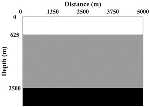
FIGURE 5. A three-layer velocity model with two flat reflectors.

FIGURE 6

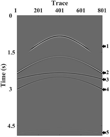
FIGURE 6. The simulated common shot gather. Arrows 1,2,4 represent the primary, first-order multiple and second-order multiple associated with the first layer. Arrows 3,5 represent the primary and first-order multiple waves associated with the second layer.

We use the cross-correlation imaging conditions to image primaries and multiples from seismic records (as shown in Figure 6). The corresponding stacked migration results are shown in Figure 7, which can not only have correct imaging at a depth of the reflectors but also produce two types of crosstalk at the wrong locations.

FIGURE 7

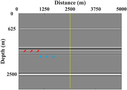
FIGURE 7. The migration result using primaries and multiples. The light blue arrows and the red arrows indicate causal crosstalk and anti-causal crosstalk, respectively.

In Figures 6, 7, the actual image of the first layer is generated by the primary and multiples of adjacent orders (arrows 1 and 2, arrows 2 and 3) reflected from the first layer based on the cross-correlation conditions. Similarly, the actual image of the second layer is generated by the primary and multiples of adjacent orders (arrows 3 and 5) reflected from the second layer based on the cross-correlation conditions. For the two types of crosstalk, arrows 1 and 4 are respectively used as virtual source wavefield and receiver wavefield to generate causal crosstalk (as light blue arrows indicate); arrows 1 and 3 are respectively used as virtual source wavefield and receiver wavefield to generate anti-causal crosstalk (as red arrows indicate).

To verify our derived equations, we extracted the angle gathers at 2.5 km (yellow dotted line in Figure 7) and stacked the analytic solutions of the derived equations onto the angle gathers obtained after migration. Figure 8 shows the angle gathers, which are extracted from the stacked imaging results after migration.

FIGURE 8

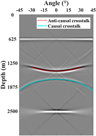
FIGURE 8. Two types of crosstalk in angle gathers. The red solid and the light blue line represent the calculated anti-causal crosstalk and causal crosstalk, respectively.

In Figure 8, we notice that the actual imaging events are horizontal in the angle domain, while the crosstalk events are curved. Moreover, the derived analytical solutions (as red and light blue curves indicate) and the actual curves of the crosstalk can be fitted well, which proves the correctness of our method. We use the subsurface offset-to-angle algorithm to obtain angle gathers; thus, the half-aperture angle γ for crosstalk is related to the offset. In this model, the maximum offset at the surface is 2.5 km, and it can be calculated that the maximum value of the analytical solution curve for causal crosstalk (as the light blue curve indicates) corresponding to the angle gathers is 45°, while the maximum value of the analytical solution curve for anti-causal crosstalk (as red curve indicates) corresponds to only 30°.

2.2 The attenuation of crosstalk in the radon domain

In the Radon domain, the imaging events and crosstalk in angle gathers can be effectively distinguished. This is because the imaging events in angle gathers are well-focused in the Radon domain, which makes it easy to separate the crosstalk in angle gathers. To separate imaging events and crosstalk more accurately in the Radon domain, we apply the two types of RMO equations derived above as new kernel functions to the Radon transform. Finally, we proved the accuracy of our derived RMO equations using model simulations.

The generic expression for the Radon transform in the angle domain (Sava and Guitton, 2005) can be expressed as:

$z\left(q,\gamma \right)=z_0+qg\left(\gamma \right),(13)$

where γ is the half-aperture angle, z₀ is the depth when γ is zero, q is a curvature parameter, and g(γ) is a function that approximates the residual moveout of the crosstalk in angle gathers.

Wang et al. (2014) performed the Radon transform on angle gathers by applying the principle of Eq 13 and used the tangent square approximation equation as the kernel function, which can be expressed as (Biondi and Symes, 2004; Sava and Guitton, 2005; Alvarez et al., 2007)

$g\left(\gamma \right)=\tan {}^2\gamma .(14)$

This approach using Eq 14 as the kernel function can separate the imaging events from the crosstalk by focusing on different curvature portions in the Radon domain. By removing the curvature portion associated with the crosstalk and stacking the results in angle gathers after the inverse Radon transform, the final imaging results can be recovered. However, Eq 14 is not derived based on the generation mechanism of crosstalk, which may influence the capability of focusing crosstalk in the Radon domain. Therefore, we use two more approximate RMO equations as new kernel functions based on Eqs 6–12, which can be expressed as:

$g_{anti-causal}\left(\gamma \right)=-\rho +\frac{\left({\rho }^2-1\right)\sin \gamma \tan \gamma -{\rho }^2\cos \gamma }{\sqrt{{\rho }^2-\sin {}^2\gamma }},(15)$

$g_{causal}\left(\gamma \right)=\frac{\cos \gamma \left({\rho }^2-\tan {}^2\gamma \left(1-{\rho }^2\right)\right)}{\sqrt{\rho 2-\sin {}^2\gamma }}-\rho ,(16)$

where Eqs 15, 16 are the RMO equation for anti-causal crosstalk and causal crosstalk, respectively.

Figure 9 displays the comparison of the tangent-squared approximation equation and two RMO equations in the angle domain. Compared to the tangent-square approximation, Eqs 15, 16 provide a more accurate description of the kinematic shape for crosstalk in angle gathers (Figures 9A, C). To show this difference, we make the relative error of the two derived RMO equations with the tangent square approximation with increasing angle (Figures 9B, D), respectively. Note that when the aperture angle is small, both derived RMO equations and the tangent-squared approximation can fit the actual curves. However, as the aperture angle increases, the derived RMO equations can better fit the actual curves as shown in Figures 9A, C. We use the two RMO equations and tangent square approximation equation as kernel functions to apply the Radon transform for angle gathers, and the results are shown in Figure 10.

FIGURE 9

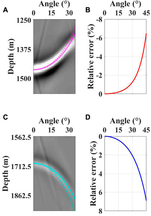
FIGURE 9. Comparison of the tangent-squared approximation equation and two RMO equations in the angle domain. (A) and (C) are the curves corresponding to the tangent-squared approximation equation and RMO equation for anti-causal and causal crosstalk in angle gathers, respectively. (B,D) are the relative error of the tangent-squared approximation to the more accurate RMO equation for anti-causal and causal crosstalk, respectively. The solid pink line and the pink dashed line represent the results of the derived RMO equation for anti-causal crosstalk and the tangent-squared approximation equation in angle gathers. The light blue solid line and the light blue dashed line represent the results of the derived RMO equation for causal crosstalk and the tangent-squared approximation equation in angle gathers.

FIGURE 10

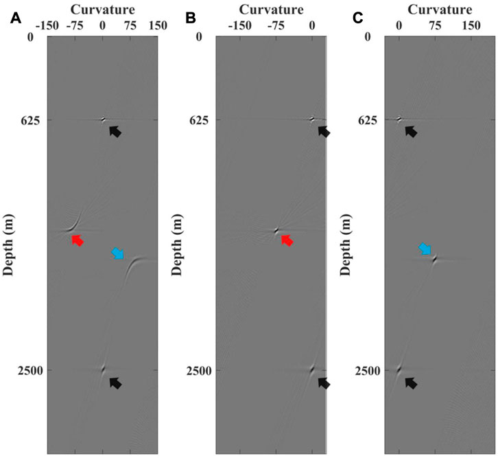
FIGURE 10. Comparison of Radon transform for angle gathers using tangent square approximation and two RMO equations. (A) Results of Radon transform for two types of crosstalk using tangent square approximation equation as kernel function, (B) Results of Radon transform for anti-causal crosstalk using derived RMO equation of anti-causal crosstalk as kernel function, (C) Results of Radon transform for causal crosstalk using derived RMO equation of causal crosstalk as the kernel function. The black arrows indicate the location of the actual imaging in the Radon domain. The red arrows indicate the location of anti-causal crosstalk in the Radon domain. The blue arrows indicate the location of causal crosstalk in the Radon domain.

In Figure 10, the actual imaging results of multiples in the Radon domain are focused at zero curvature (as black arrows indicate), while the crosstalk events are focused at non-zero curvature (as light blue arrows and red arrows indicate). In addition, the results of the Radon transform for angle gathers using these two equations as kernel functions are more focused in the Radon domain (Figures 10B, D). Based on the focused capabilities, our method can separate the correct imaging and crosstalk in the Radon domain, thus recovering high signal-to-noise imaging results.

3 Numerical examples

We apply the proposed method to numerical examples. A subset of the Sigsbee2b model, as shown in Figure 11, is used to test the feasibility and robustness of our method.

FIGURE 11

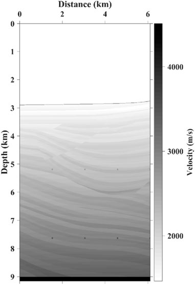
FIGURE 11. The Sigsbee2b velocity model.

The subset of the Sigsbee2b model has 801 grid points in the horizontal direction and 1,201 grid points in the vertical direction, and the grid size is 7.62 m. The velocity model used for producing seismic records is shown in Figure 11, which contains the faults portion of the Sigsbee2b model. A Ricker wavelet with a dominant frequency of 25 Hz and a maximum frequency of 45 Hz is employed to mimic a P-wave source. The number of shots is 125, with a shot interval of 48.72 m and a receiver interval of 22.86 m. For one shot gather, we deploy both the sources and receivers at the surface with minimum and maximum offsets of 0 m and 6,096 m. Split-spread acquisition geometry is used for numerical simulation. The length of the data record is 20 s, and the time sample interval is 0.8 ms. The seismic records with direct waves and ghost waves are removed for imaging of multiples.

The Sisgbee2b model has a high-velocity reflector at the bottom, which can produce multiples with strong amplitudes. We use the one-way wave-equation migration algorithm for the imaging of multiples. Figure 12 shows the imaging result for the subset of the Sigsbee2b model. From the comparison of the imaging result (Figure 12) with the actual Sigsbee2b velocity model (Figure 11), it can be seen that not only the correct imaging events are generated, but also events are generated at the wrong locations. Similar to the model in Figure 1, these wrong events, i.e., crosstalk, are generated by primaries and multiples related to the water bottom and the bottom reflector of the Sigsbee2b model based on the cross-correlation imaging conditions. In Figure 12, the red arrows indicate the anti-causal crosstalk event, which is related to the bottom of the Sigsbee2b model, and the light blue arrows indicate the causal crosstalk event, which is related to the water bottom. Note that these two types of crosstalk are not much different from the actual imaging events in terms of characteristics, which can be challenging to attenuate crosstalk in the imaging results. Moreover, the two above have different moveouts in the angle domain, and the crosstalk events are more separable. Therefore, to show the difference between crosstalk events and effective imaging, we apply the subsurface offset-angle conversion algorithm to compute the angle gathers after migration.

FIGURE 12

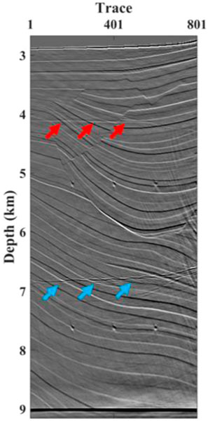
FIGURE 12. The imaging results of migration. The red arrows and light blue arrows mark the locations of anti-causal crosstalk and causal crosstalk, respectively.

Figure 13 shows the angle gathers of the 201st, 401st, 601st, and 801st seismic traces. The imaging angle range in each angle gather is from −45° to 45° with a sampling of 0.5°. In Figure 13, the crosstalk events are curved in the angle domain, while the actual imaging is flat. In addition, the crosstalk events display different bending patterns due to their kinematic mechanisms. Among them, the curve that bends upward is anti-causal crosstalk (as red arrows indicate), and the curve that bends downward is causal crosstalk (as light blue arrows indicate). As discussed in the preceding section, the Radon transform can separate these two crosstalk events from the effective imaging and thus achieve the purpose of attenuating the crosstalk. By using the RMO equations for two types of crosstalk previously obtained as the kernel functions for the Radon transform and by performing the Radon transform on the obtained angle gathers, we can separate the crosstalk and the actual imaging in the Radon domain.

FIGURE 13

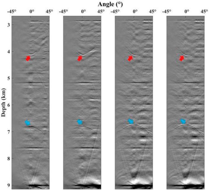
FIGURE 13. Angle gathers after migration. The red arrows and light blue arrows mark the locations where the anti-causal crosstalk and the causal crosstalk are located, respectively.

Figure 14 shows the results of the Radon transform using two kernel functions for trace 401 of ADCIGs. In Figure 14, the actual imaging is focused on the zero-curvature portion, while the anti-causal crosstalk and the causal crosstalk are respectively distributed on the left (as the red arrow indicates in Figure 14A) and right sides (as the light blue arrow indicates in Figure 14B) of the zero-curvature portions in the Radon domain. In this domain, the two types of crosstalk and effective imaging correspond to three different curvature components, respectively. The results of the radon transform in Figure 14 show that our method can significantly separate crosstalk and the correct imaging in the Radon domain when facing complex reflectors. Therefore, the effective imaging results in the Radon domain can be obtained by removing the non-zero curvature components in Figures 14A, B with a suitable function. Next, we transfer the effective images in the Radon domain to the angle domain by inverse Radon transform and stack the angle gathers of 801 traces to obtain the imaging results with crosstalk attenuated.

FIGURE 14

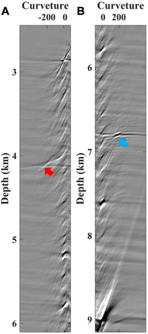
FIGURE 14. Results in radon domain after radon transform with two kernel functions. (A) The Radon transform using the RMO equation of anti-causal crosstalk as the kernel function, (B) the Radon transform using the RMO equation of causal crosstalk as the kernel function. The red arrows and light blue arrows mark the locations where the anti-causal crosstalk and the causal crosstalk are located, respectively.

Figure 15 shows the imaging result after attenuating crosstalk events. Compared with the imaging results without crosstalk attenuation (Figure 12), the imaging results in Figure 15 have better resolution with two types of crosstalk attenuated. In addition, some of the less obvious crosstalk events are also attenuated to some extent. In summary, the proposed method to attenuate crosstalk for imaging of multiples can be used for complex models, which demonstrates the feasibility and robustness of our proposed method.

FIGURE 15

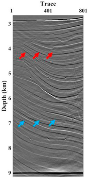
FIGURE 15. Denoised migration result. The red and light blue arrows mark the positions of the two types of crosstalk before being denoised.

4 Conclusion

To solve the problem of unphysical kernel functions when applying the Radon transform to remove crosstalk in the angle domain, we derive two RMO equations for crosstalk based on the causality and apply them to attenuate crosstalk in the Radon domain. The RMO equations can accurately describe the kinematic mechanism of the crosstalk in the angle domain. A simple model verifies the accuracy of the RMO equations. Compared with the Radon transform using the conventional tangent-squared approximation, our equations can make the crosstalk more focused in the Radon domain and can better separate the crosstalk from the actual imaging. A subset of the Sigsbee2b model is used for the numerical test, and it has validated the feasibility and robustness of our method. The crosstalk attenuated using our method has recovered high signal-to-noise imaging results, which benefits the subsequent geological interpretation. In our paper, we use the subsurface offset-to-angle algorithm to obtain ADCIGs, therefore, for 3D seismic data, we need to face the challenge of extracting ADCIGs more efficiently to address a large number of calculations. In addition, our approach assumes that the source ghost and receiver ghost do not exist. Therefore, in practical seismic data processing, this situation may have an influence on the accuracy of crosstalk attenuation.

Data availability statement

The raw data supporting the conclusion of this article will be made available by the authors, without undue reservation.

Author contributions

ZG and SZ contributed to the methodology and wrote the original draft of the paper. SL contributed to the conceptualization and supervision. Data analysis was conducted by HW and KR. All authors reviewed the final submitted version of the manuscript.

Funding

This study is partially funded by the National Natural Science Foundation of China (grant no. 42074123), National Natural Science Foundation of China (grant no. 42230805) and the Pearl River Talent Program of Guangdong, China (grant no. 2017ZT07Z066).

Acknowledgments

Our great gratitude goes to the reviewers Yike Liu, Jianping Huang, Weijia Sun and the editor Qizhen Du. Their careful work and thoughtful suggestions helped greatly improve this paper.

Conflict of Interest

The authors declare that the research was conducted in the absence of any commercial or financial relationships that could be construed as a potential conflict of interest.

Publisher’s note

All claims expressed in this article are solely those of the authors and do not necessarily represent those of their affiliated organizations, or those of the publisher, the editors and the reviewers. Any product that may be evaluated in this article, or claim that may be made by its manufacturer, is not guaranteed or endorsed by the publisher.

References

Alvarez, G., Biondi, B., and Guitton, A. (2007). Attenuation of specular and diffracted 2D multiples in image space. GEOPHYSICS 72, V97–V109. doi:10.1190/1.2759439

CrossRef Full Text | Google Scholar

Berkhout, A. J. G. (2014). Review paper: An outlook on the future of seismic imaging, Part I: Forward and reverse modelling. Geophys. Prospect. 62, 911–930. doi:10.1111/1365-2478.12161

CrossRef Full Text | Google Scholar

Berkhout, A. J., and Verschuur, D. J. (2003). “Transformation of multiples into primary reflections,” in SEG technical Program expanded abstracts 2003 (Tulsa: Society of Exploration Geophysicists), 1925–1928. doi:10.1190/1.1817697

CrossRef Full Text | Google Scholar

Berkhout, A. J., and Vershuur, D. J. (1994). “Multiple technology: Part 2, migration of multiple reflections,” in SEG technical Program expanded abstracts 1994 (Tulsa: Society of Exploration Geophysicists), 1497–1500. doi:10.1190/1.1822821

CrossRef Full Text | Google Scholar

Biondi, B., and Symes, W. W. (2004). Angle-domain common-image gathers for migration velocity analysis by wavefield-continuation imaging. GEOPHYSICS 69, 1283–1298. doi:10.1190/1.1801945

CrossRef Full Text | Google Scholar

Gu, Z., and Wu, R.-S. (2022). Internal multiple removal and illumination correction for seismic imaging. IEEE Trans. Geosci. Remote Sens. 60, 1–11. doi:10.1109/TGRS.2021.3080210

CrossRef Full Text | Google Scholar

Liu, Y., Chang, X., Jin, D., He, R., Sun, H., and Zheng, Y. (2011). Reverse time migration of multiples for subsalt imaging. Geophysics 76 (5), WB209–WB216. doi:10.1190/geo2010-0312.1

CrossRef Full Text | Google Scholar

Liu, Y., Liu, X., Osen, A., Shao, Y., Hu, H., and Zheng, Y. (2016). Least-squares reverse time migration using controlled-order multiple reflections. GEOPHYSICS 81, S347–S357. doi:10.1190/geo2015-0479.1

CrossRef Full Text | Google Scholar

Lu, S., Liu, F., Chemingui, N., Valenciano, A., and Long, A. (2018). Least-squares full-wavefield migration. Lead. Edge 37, 46–51. doi:10.1190/tle37010046.1

CrossRef Full Text | Google Scholar

Lu, S., Qiu, L., and Li, X. (2021). Addressing the crosstalk issue in imaging using seismic multiple wavefields. GEOPHYSICS 86, S235–S245. doi:10.1190/geo2020-0364.1

CrossRef Full Text | Google Scholar

Lu, S., Whitmore, N., Valenciano, A., Chemingui, N., and Ronholt, G. (2016). “A practical crosstalk attenuation method for separated wavefield imaging,” in SEG technical Program expanded abstracts 2016 (Dallas, Texas: Society of Exploration Geophysicists), 4235–4239. doi:10.1190/segam2016-13849878.1

CrossRef Full Text | Google Scholar

Ordoñez, A., Söllner, W., Klüver, T., and Gelius, L. J. (2014). Migration of primaries and multiples using an imaging condition for amplitude-normalized separated wavefields. GEOPHYSICS 79, S217–S230. doi:10.1190/geo2013-0346.1

CrossRef Full Text | Google Scholar

Sava, P. C., and Fomel, S. (2003). Angle-domain common-image gathers by wavefield continuation methods. GEOPHYSICS 68, 1065–1074. doi:10.1190/1.1581078

CrossRef Full Text | Google Scholar

Sava, P., and Guitton, A. (2005). Multiple attenuation in the image space. GEOPHYSICS 70, V10–V20. doi:10.1190/1.1852789

CrossRef Full Text | Google Scholar

Schuster, G. T., and Rickett, J. (2000). Daylight imaging in V(x, y, z) media. Utah tomography and modeling-migration: Project midyear report, 55–66.

Google Scholar

Singh, S., Snieder, R., van der Neut, J., Thorbecke, J., Slob, E., and Wapenaar, K. (2017). Accounting for free-surface multiples in Marchenko imaging. GEOPHYSICS 82, R19–R30. doi:10.1190/geo2015-0646.1

CrossRef Full Text | Google Scholar

Tu, N., and Herrmann, F. J. (2015). Fast imaging with surface-related multiples by sparse inversion. Geophys. J. Int. 201, 304–317. doi:10.1093/gji/ggv020

CrossRef Full Text | Google Scholar

Wang, Y., Zheng, Y., Zhang, L., Chang, X., and Yao, Z. (2014). Reverse time migration of multiples: Eliminating migration artifacts in angle domain common image gathers. GEOPHYSICS 79, S263–S270. doi:10.1190/geo2013-0441.1

CrossRef Full Text | Google Scholar

Wapenaar, K., Thorbecke, J., van der Neut, J., Broggini, F., Slob, E., and Snieder, R. (2014). Marchenko imaging. GEOPHYSICS 79, WA39–WA57. doi:10.1190/geo2013-0302.1

CrossRef Full Text | Google Scholar

Wong, M., Biondi, B. L., and Ronen, S. (2015). Imaging with primaries and free-surface multiples by joint least-squares reverse time migration. GEOPHYSICS 80, S223–S235. doi:10.1190/geo2015-0093.1

CrossRef Full Text | Google Scholar

Xu, S., Zhang, Y., and Tang, B. (2011). 3D angle gathers from reverse time migration. GEOPHYSICS 76, S77–S92. doi:10.1190/1.3536527

CrossRef Full Text | Google Scholar

Yoon, K., and Marfurt, K. J. (2006). Reverse-time migration using the poynting vector. Explor. Geophys. 37, 102–107. doi:10.1071/EG06102

CrossRef Full Text | Google Scholar

Zhang, D., and Schuster, G. T. (2014). Least-squares reverse time migration of multiples. GEOPHYSICS 79, S11–S21. doi:10.1190/geo2013-0156.1

CrossRef Full Text | Google Scholar