An explicit stable Q-compensated reverse time migration scheme for complex heterogeneous attenuation media

Prestack reverse-time migration (RTM) is a popular imaging technique for complex geological conditions, since the amplitude attenuation and velocity dispersion are common in seismic recordings. To image attenuated seismic recordings accurately, a robust migration algorithm with a stable attenuation compensation approach should be considered. In the context of the Q-compensated RTM approach based on the decoupled fractional Laplacians (DFLs) viscoacoustic wave equation, amplitude compensation can be implemented by flipping the sign of the dissipation term. However, the non-physical magnification of image amplitude could lead to a well-known numerical instability problem. The explicit stabilization operator can rectify the amplitude attenuation and suppress the numerical instability. However, limited by the inconvenient mixed-domain operator, the average Q value rather than the real Q value is often used in the compensation operator, lowering the compensated accuracy of the migration image. To overcome this problem, we propose a novel explicit Q-compensation scheme. The main advantage of the proposed compensation operator is that its order is space-invariant, making it more suitable for handling complex heterogeneous attenuation media. Several two-dimensional (2D) and three-dimensional (3D) synthetic models are used to verify the superiority of the proposed approach in terms of amplitude fidelity and image resolution. Field data further demonstrates that our approach has potential applications and can greatly enhance the resolution of seismic images.

Introduction

Seismic attenuation is commonly observed in the rock matrix and pores such as sandstones and gas clouds (Aki and Richards, 1980; Dutta and Schuster, 2014), which is commonly characterized by the quality factor Q (Tselentis, 1998). The inherent attenuation properties of the Earth media significantly affect the characteristics of seismic waves in terms of amplitude, phase, and frequency band (Carcione, 1990; Zhu et al., 2013; Yang et al., 2015). As accurate attenuation compensation is critical for understanding the mechanisms of seismic data and mapping the Earth’s interior, ignoring the anelasticity would result in blurred migrated images, dimmed amplitudes, and ultimately reduce the reliability of seismic interpretation (Wang and Guo, 2004; Zhang and Gao, 2021). Currently, the Q-compensated schemes are divided into two categories. The first method is usually implemented on the post-stack seismic profile, such as the inverse-Q filtering method (Bickel and Natarajan, 1985; Wang, 2002; Wang, 2003), time-variant spectral whitening (Yilmaz, 2001), and time-varying deconvolution (Margrave et al., 2011). Although these methods are computationally efficient, they are usually suitable for simple structures because of the lack of consideration for the internal physical connotation in the process of wave propagation (Hargreaves and Calvert, 1991). The second approach is based on wave equations and compensates for attenuation along the propagation path (Dai and West, 1994; Mittet, 2007; Li et al., 2016b). Since the attenuation occurs during wave propagation, it is more reasonable to implement Q-compensated as part of the migration process (Zhang et al., 2010; Zhu and Sun, 2017; Zhao Y. et al., 2018).

Earth materials usually exhibit nearly frequency-independent Q behavior over the seismic frequency band (Korneev et al., 2004; Dvorkin and Mavko, 2006; Zhu, 2017). Mechanical models are the most commonly used approaches for describing frequency-independent Q behavior (Mainardi, 2010; Rossikhin, and Shitikova, 2010). Among these, the standard linear solid (SLS) and the generalized standard linear solid (GSLS) models have been extensively used in modeling and imaging (Xu and McMechan, 1995; Causse and Ursin, 2000; Deng and McMechan, 2008; Zhang and Gao, 2022). Alternatively, some mathematical-model-based schemes, such as the Kolsky-Margravechen model (Kolsky, 1956; Futterman, 1962), the power-law model, and Kjartansson’s constant-Q model (Kjartansson, 1979; Zhu and Bai, 2018; Wang et al., 2020), are also gradually applied to the characterization of Earth attenuation. Recently, the decoupled fractional Laplacians (DFL) viscoacoustic wave equation has attracted attention (Chen et al., 2016; Yao et al., 2016; Wang N. et al., 2018; Xing and Zhu, 2019; Liu and Luo, 2021) for the following reasons. First, it incorporates the spatial fractional Laplacians to avoid the memory issue often encountered by conventional anelastic modeling (Dutta and Schuster, 2014) and fractional time derivative approaches (Carcione, 2008). Second, compared with SLS, this strategy is more attractive for Q-RTM because it realizes amplitude compensation by flipping the sign of the amplitude-loss term without changing phase information (Guo and McMechan, 2015; Guo et al., 2016).

Attenuation compensation is critical for improving imaging quality in complex attenuation structures. However, Q-RTM usually suffers from numerical instability due to the inverse-physical energy amplification of high-frequency noise. Several strategies have been proposed to improve numerical stability. For example, the schemes include regularization approaches (Zhang et al., 2010; Wang et al., 2012), filter-based approaches (Zhu and Harris, 2014; Wang Y. et al., 2018; Chen et al., 2020a), improved imaging conditions (Xie et al., 2015; Zhao X. H. et al., 2018; Sun and Zhu, 2018; Yang et al., 2021) and least-squares Q reverse-time migration (QLSRTM) (Chen et al., 2020b; Zhang et al., 2022; Zhang and Gao, 2022). Among these, the implicit adaptive stabilization compensation scheme (Wang et al., 2017) that adjusts the truncation frequency according to the propagation time and Q value provides a better trade-off between numerical stability and imaging resolution. However, the implicit compensation operator is calculated in the wavenumber domain, implying that it requires additional Fourier transforms. Wang et al. (2019) further proposed an explicit compensation strategy, which adjusts compensation parameters more conveniently and simplifies the workflow of Q-RTM. Nevertheless, this strategy is not straightforward for dealing with the complex heterogeneous Q media (Sun and Zhu, 2015) because it involves the spatial variable-order Laplacians (mixed-domain operators). To solve the mixed-domain problem, the average Q value is usually used to replace the real Q value (Wang et al., 2019), which would introduce significant errors for the sharp Q-contrast models (Chen et al., 2016; Yang and Zhu, 2018a; Xing and Zhu, 2019).

In this study, we aim to derive a new explicit Q-compensated scheme so as to accurately image complex heterogeneous attenuation structures. Our derivation seeks an equation that avoids calculating spatial variable-order Laplacian operators starting from the explicit compensation wave equation (Wang et al., 2019). To accomplish this, we used Taylor expansion to approximate the spatial variable-order Laplacian operators to the spatial constant-order form and then integrate the constant-order compensated scheme into the Q-RTM framework. The following are the advantages of the proposed method. First, the proposed scheme enables us to compensate for amplitude loss in Q-RTM without changing the phase because the dispersion and dissipation effects are naturally separated. Second, the explicit Q-compensated scheme is free from frequent Fourier transforms, so it is expected to simplify the workflow of Q-RTM. Third, compared with the original compensation operator with average Q, the proposed algorithm visibly improves the imaging quality in the heterogeneous Q media.

The organization of this study is as follows. First, we review the explicit Q-compensation wave equation with spatial variable-order Laplacian operators (Wang et al., 2019; Wang et al., 2022). Second, we demonstrate the derivation of the proposed spatial constant-order Q-compensated wave equation, followed by detailing its numerical implementation and validating its accuracy. Then, much synthetic and field data are used to demonstrate its advantages. Finally, we conduct a discussion and draw some conclusions.

Materials and methods

Constant-order compensated viscoacoustic wave equation.

According to a previous study (Wang et al., 2019; Wang et al., 2021), the wave equation based on the explicit compensated operators can be expressed as follows:

$\frac{1}{c^2}\frac{{\partial }^{2}p}{\partial t^2}={\eta }_a+{\tau }_a+{\eta }_{c1}+{\eta }_{c2}+{\tau }_c(1)$

and

$\left\{\begin{array}{l}{\eta }_a=-c_0^{2\gamma }{\omega }_0^{-2\gamma }\cos \left(\pi \gamma \right){\left(-{\nabla }^2\right)}^{\gamma +1}p,{\tau }_a=c_0^{2\gamma -1}{\omega }_0^{-2\gamma }\sin \left(\pi \gamma \right)\frac{\partial }{\partial t}{\left(-{\nabla }^2\right)}^{\gamma +0.5}p,\\ {\eta }_{c1}=c_0^{2\gamma -1}{\omega }_0^{-2\gamma }\sin \left(\pi \gamma \right)\sigma {\left(-{\nabla }^2\right)}^{\left(2\gamma +1+\beta \right)/2}p,{\eta }_{c2}=-\frac{{\sigma }^2}{c^2}{\left(-{\nabla }^2\right)}^{\beta }p,\\ {\tau }_c=-\frac{2\sigma }{c^2}\frac{\partial }{\partial t}{\left(-{\nabla }^2\right)}^{\beta /2}p,\gamma =\frac{1}{\pi Q},c=c_0\cos \left(\pi \gamma /2\right),\end{array}\right.(2)$

where $c_0$ is the phase velocity at the reference frequency ${\omega }_0$. $p$ and ${\nabla }^2$ represent the pressure wavefield and Laplacian operator, respectively. ${\eta }_a$ and ${\tau }_a$ represent phase dispersion and amplitude compensation terms, respectively. ${\eta }_{c1}$ and ${\eta }_{c2}$ is introduced to keep the phase unchanged during Q compensation. ${\tau }_c$ is a stabilization term to keep the high-wavenumber component from uncontrolled amplification, in which $\beta$ and $\sigma$ are the stable compensation parameters. The stable compensation parameters usually depend on the media’s physical properties. Generally, A larger $\beta$ can reserve more higher frequency, and the more high-wavenumber signal is eliminated with $\sigma$ increases (Wang et al., 2021).

Equation 1 can compensate for amplitude without introducing high-frequency noise because it includes the stabilization term. However, subject to the thorny mixed-domain (spatial-wavenumber domain) operators, the average Q value is often used when extrapolating the wavefields (Zhu et al., 2014; Zhu and Harris, 2014; Mu et al., 2021). Even though the average scheme works well for the homogeneous or smooth Q model, it cannot accurately describe the characteristics of wave propagation in the heterogeneous media (Yang and Zhu, 2018b). To overcome this shortcoming, we propose a new explicit viscoacoustic wave equation with the constant fractional-order Laplacians using a truncated Taylor expansion algorithm (Chen et al., 2016).

If seismic waves propagate in a homogeneous medium, the plane wave equation is substituted into Eq. 1 to obtain the frequency-wavenumber domain viscoacoustic wave equation

$\frac{1}{c^2\cos \left(\pi \gamma \right)}\frac{{\partial }^2\stackrel{\sim }{p}}{\partial t^2}={\stackrel{\sim }{\eta }}_a+{\stackrel{\sim }{\tau }}_a+{\stackrel{\sim }{\eta }}_{c1}+{\stackrel{\sim }{\eta }}_{c2}+{\stackrel{\sim }{\tau }}_c,(3)$

and

$\left\{\begin{array}{l}{\stackrel{\sim }{\eta }}_a=-c_0^{2\gamma }{\omega }_0^{-2\gamma }{k}^{2\gamma +2}\stackrel{\sim }{p},{\stackrel{\sim }{\tau }}_a=c_0^{2\gamma -1}{\omega }_0^{-2\gamma }\frac{1}{Q}{k}^{2\gamma +1}\frac{\partial \stackrel{\sim }{p}}{\partial t},\\ {\stackrel{\sim }{\eta }}_{c1}=c_0^{2\gamma -1}{\omega }_0^{-2\gamma }\frac{\sigma }{Q}{k}^{2\gamma +1+\beta }\stackrel{\sim }{p},{\stackrel{\sim }{\eta }}_{c2}=-\frac{{\sigma }^2{k}^{2\beta }}{c^2\cos \left(\pi \gamma \right)}\stackrel{\sim }{p},\\ {\stackrel{\sim }{\tau }}_c=-\frac{2\sigma k^{\beta }}{c^2\cos \left(\pi \gamma \right)}\frac{\partial \stackrel{\sim }{p}}{\partial t}\end{array}\right.(4)$

where $\stackrel{\sim }{p}$ represents the wavefield in the wavenumber domain. Here, the fractional Laplacian $c_0^{2\gamma -1}{\omega }_0^{-2\gamma }\frac{\sigma }{Q}{k}^{2\gamma +1+\beta }$ in Eq. 3 is taken as an example of an approximation

$c_0^{2\gamma -1}{\omega }_0^{-2\gamma }\frac{\sigma }{Q}{k}^{2\gamma +1+\beta }=\frac{\lambda \sigma }{Q{c}_0}{k}^{1+\beta }{\left(\frac{k}{k_d}\right)}^{2\gamma }(5)$

where $f_d$ and $k_d$ represent the dominant frequency and dominant wave number, respectively, $\lambda ={\left({\omega }_d/{\omega }_0\right)}^{2\gamma }$, ${\omega }_d=2\pi f_d$. Because $2\gamma \left|\ln \frac{k}{k_d}\right|\ll 1$, we use Taylor expansion to approximate Eq. 3 as

$\frac{\lambda \sigma }{Q{c}_0}{k}^{1+\beta }{\left(\frac{k}{k_d}\right)}^{2\gamma }\approx \frac{\lambda \sigma }{Q{c}_0}{k}^{1+\beta }\left(1+2\gamma \ln \frac{k}{k_d}\right),(6)$

$1+2\gamma \ln \frac{k}{k_d}$ can be approximated by Taylor expansion again

$1+2\gamma \ln \frac{k}{k_d}=1+\frac{2\gamma }{\zeta }\ln \left(1+{\left(\frac{k}{k_d}\right)}^{\zeta }-1\right)\approx 1+\frac{2\gamma }{\zeta }\left({\left(\frac{k}{k_d}\right)}^{\zeta }-1\right),(7)$

where $\zeta$ is a empirical constant coefficient (Chen et al., 2016), which is introduced to guarantee ${\left(\frac{k}{k_d}\right)}^{\zeta }-1$ close to zero. Therefore, the left-hand side of Eq. 5 can be approximated as follows:

$c_0^{2\gamma -1}{\omega }_0^{-2\gamma }\frac{\sigma }{Q}{k}^{2\gamma +1+\beta }\approx \frac{\lambda \sigma }{Q{c}_0}{k}^{1+\beta }\left(1+\frac{2\gamma }{\zeta }\left({\left(\frac{k}{k_d}\right)}^{\zeta }-1\right)\right)(8)$

The other spatial variable-order Laplacians in Eq. 4 can be approximated in the same way. Therefore, Eq. 3 can be expressed as follows:

$\frac{1}{\lambda c^2\cos \left(\pi \gamma \right)}\frac{{\partial }^2\stackrel{\sim }{p}}{\partial t^2}={\stackrel{\sim }{\eta }}_{anew}+{\stackrel{\sim }{\tau }}_{anew}+{\stackrel{\sim }{\eta }}_{cnew}+\frac{1}{\lambda \cos \left(\pi \gamma \right)}{\stackrel{\sim }{\eta }}_{c2}+\frac{1}{\lambda \cos \left(\pi \gamma \right)}{\stackrel{\sim }{\tau }}_c(9)$

where

$\left\{\begin{array}{l}{\stackrel{\sim }{\eta }}_{anew}=-\left(1-\frac{2}{\xi \pi Q}\right)k^2\stackrel{\sim }{p}-\frac{2}{\xi \pi Q}{\left(\frac{c_0}{{\omega }_d}\right)}^{\xi }{k}^{1+0.5\xi }\stackrel{\sim }{p},\\ {\stackrel{\sim }{\tau }}_{anew}=\frac{1}{Q{c}_0}\frac{\partial }{\partial t}\left(\left(1-\frac{2}{\xi \pi Q}\right)k^{0.5}+\frac{2}{\xi \pi Q}{\left(\frac{c_0}{{\omega }_d}\right)}^{\xi }{k}^{0.5+0.5\xi }\right)\stackrel{\sim }{p},\\ {\stackrel{\sim }{\eta }}_{cnew}=\frac{\sigma }{Q{c}_0}\left(\left(1-\frac{2}{\xi \pi Q}\right)k^{\left(1+\beta \right)/2}+\frac{2\sigma }{\xi \pi Q}{\left(\frac{c_0}{{\omega }_c}\right)}^{\zeta }{k}^{\left(\xi +1+\beta \right)/2}\right)\stackrel{\sim }{p},\end{array}\right.(10)$

By transforming Eq. 9 back to the space domain, we obtain the following equation

$\frac{1}{\lambda c^2\cos \left(\pi \gamma \right)}\frac{{\partial }^{2}p}{\partial t^2}={\eta }_{anew}+{\tau }_{anew}+{\eta }_{cnew}+\frac{1}{\lambda \cos \left(\pi \gamma \right)}{\eta }_{c2}+\frac{1}{\lambda \cos \left(\pi \gamma \right)}{\tau }_c(11)$

where

$\left\{\begin{array}{l}{\eta }_{anew}=\left(1-\frac{2}{\xi \pi Q}\right){\nabla }^{2}p-\frac{2}{\xi \pi Q}{\left(\frac{c_0}{{\omega }_d}\right)}^{\xi }{\left(-{\nabla }^2\right)}^{1+0.5\xi }p,\\ {\tau }_{anew}=\frac{1}{Q{c}_0}\frac{\partial }{\partial t}\left(\left(1-\frac{2}{\xi \pi Q}\right){\left(-{\nabla }^2\right)}^{0.5}+\frac{2}{\xi \pi Q}{\left(\frac{c_0}{{\omega }_d}\right)}^{\xi }{\left(-{\nabla }^2\right)}^{0.5+0.5\xi }\right)p,\\ {\eta }_{cnew}=\frac{\sigma }{Q{c}_0}\left(\left(1-\frac{2}{\xi \pi Q}\right){\left(-{\nabla }^2\right)}^{\left(1+\beta \right)/2}+\frac{2\sigma }{\xi \pi Q}{\left(\frac{c_0}{{\omega }_d}\right)}^{\xi }{\left(-{\nabla }^2\right)}^{\left(\xi +1+\beta \right)/2}\right)p.\end{array}\right.(12)$

In Eq. 11, the fractional Laplacians is the constant-order form, and it naturally adapts to sharp Q media. Note that for $Q\to \infty$ case, Eq. 11 reduces to the classic acoustic-wave equation. We introduce the general principle of Q-RTM in the framework of the proposed wave equation (Zhu, 2016; Wang et al., 2021).

Stable constant-order Q-compensated RTM framework

The complete procedure of the proposed Q-compensated RTM is summarized as follows.

Step 1. Forward extrapolating the source wavefield.Through a given source wavelet $S\left({\mathbf{x}}_s,t\right)$, we solve Eq. 11 to extrapolate the source wavefield, then checkpoint wavefields (Chen et al., 2020c) are stored. For source excitation at source positions

$p\left({\mathbf{x}}_s,t\right)=S\left({\mathbf{x}}_s,t\right)(13)$

where ${\mathbf{x}}_s$ indicate the source positions.

Step 2. Perform backward propagation at each receiver position.We solve Eq. 11 to extrapolate the receiver wavefields where the backward source is recorded data $R\left({\mathbf{x}}_r,t\right)$ in time as the boundary condition. The receivers’s excitation at the record positions is given as follows:

$p\left({\mathbf{x}}_r,t\right)=R\left({\mathbf{x}}_r,T_{\max }-t\right)(14)$

where ${\mathbf{x}}_r$ and $T_{\max }$ represent the receiver positions and record duration, respectively.

Step 3. Compute the final imaging results using an imaging condition.Finally, the zero-lag crosscorrelation imaging condition is used to obtain the image of the subsurface structure (Claerbout, 1971) as follows:

$I_p\left(\mathbf{x}\right)={\int }_0^{T_{\max }}{p}_s\left(\mathbf{x},t\right)p_r\left(\mathbf{x},t\right)dt(15)$

where $I_p\left(\mathbf{x}\right)$ represents the imaging result at position x. $p_s\left(\mathbf{x},t\right)$ and $p_r\left(\mathbf{x},t\right)$ express the compensated source and receiver wavefields, respectively. To ensure the time consistency between the source and receiver wavefields, the source wavefields should be read from the disk or reconstructed (Ren et al., 2022).

Numerical implementation

The pseudo-spectral method is widely applied to solve the fractional Laplacian operator (Xue et al., 2017; Wang et al., 2018; Wang et al., 2020; Wang et al., 2022). We used the second-order central finite-difference approach and fast Fourier transform (FFT) to calculate the temporal derivative and fractional Laplacian operators, respectively (Bai et al., 2019; Xing and Zhu, 2020; 2021). The detailed numerical implementation is summarized in the following three steps.

1) Calculate the fractional Laplacians. Take ${\left(-{\nabla }^2\right)}^{1+0.5\xi }p$ as an example, and it can be expressed as follows:

${\left(-{\nabla }^2\right)}^{1+0.5\xi }p=F^{-1}\left\{{\left({\left|\mathbf{k}\right|}^2\right)}^{1+0.5\xi }F\left[p\right]\right\}(16)$

where $F$ and $F^{-1}$ denotes the forward and inverse Fourier transform, respectively, and $\left|\mathrm{k}\right|$ is the norm of the complex wavenumber vector. $\zeta$ is an invariable coefficient defined $\zeta =1/16$ in this study (Chen et al., 2016).

2) Calculate the time partial derivative and next moment wavefields.

$p^{it+1}=2p^{it}-p^{it-1}+Lap(17)$

where $p^{it+1},p^{it},p^{it-1}$ represents the wavefields at the next, current, and previous timestep, respectively. $Lap$ denotes all Laplacians.

3) Update the wavefields and enter the next time cycle until the maximum simulation time.

Therefore, the Q-compensated wave equation based on the constant fractional-order Laplacians can be implemented.

Accuracy analysis

We conduct a numerical test to analyze this approximation accuracy because the spatial constant-order fractional Laplacian is approximated using Taylor expansion. Here, we take Eq. 8 as an example. This test is performed using a 2D homogeneous model with a grid size of 200 × 200 nodes and spatial intervals of 10 m. The reference velocity is 4,000 m/s. For simplicity, we set $\lambda =1,\zeta =1/16,\beta =1$. The degree of match between our approximation solution (the right-hand side of Eq. 8) and the original solution (left-hand side of Eq. 8) is evaluated using the relative root mean square error (RRMS) defined as follows:

$\text{RRMS}=\sqrt{{{\displaystyle \sum }_i^N\left(\left(x_{ai}-x_{bi}\right)/x_{ai}\right)}^2}/N(18)$

where $x_{ai}$ and $x_{bi}$ represent the left and right sides of Eq. 8, respectively.

Figure 1 shows the RRMS of different simulation parameters, in which Q ranges from 10 to 100 and $f_d$ (dominant frequency) ranges from 5 to 50 Hz. The value of RRMS decreases with an increase in Q (Figure 1), and it is almost unchanged as the frequency varies. Furthermore, our approximation has a small RRMS even for the lower Q, validating the accuracy of our approximation. Furthermore, we compare several numerical simulations of different wave equations to investigate the accuracy of Eq. 11 in wavefield extrapolation. A Ricker wavelet is used as the source and is located at the center of a homogeneous model. The single traces of the different wave equation wavefields at x = 1 km are shown in Figure 2, where Figures 2A–D correspond to $Q=20,f_d=20$, $Q=50,f_d=20$, $Q=20,f_d=50$, and $Q=50,f_d=50$, respectively. We can find that both types of compensation wave equations can simulate almost the same wavefields as the reference solutions (the black line, Q = infinity), confirming the validity of the compensation wave equation.

FIGURE 1

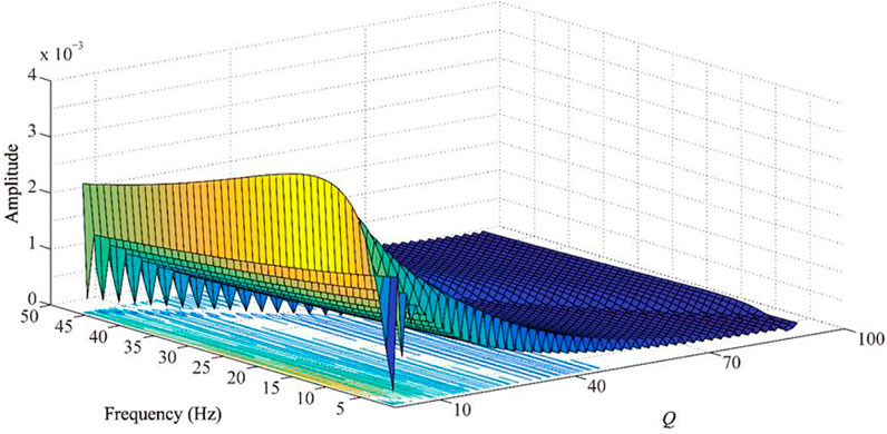
FIGURE 1. RRMS with different parameters.

FIGURE 2

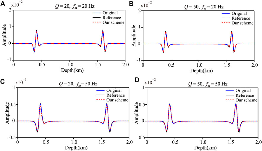
FIGURE 2. Single trace at (x = 1 km) with different wave equations. (A) $Q=20,f_m=20$; (B) $Q=50,f_m=20$; (C) $Q=20,f_m=50$; (D) $Q=50,f_m=50$.

Numerical examples

Two-layer model

Different from Wang et al. (2021) method, the proposed method avoids calculating the spatial variable-order fractional Laplacians. Therefore, it is more straightforward for dealing with the sharp Q model, which can be verified by the two-layer model (Figure 3). The grid is 400 × 400 cells with a unified 5 m interval. Ricker wavelet with a peak frequency of 30 Hz is the location in the center of the model and has a time step of 0.5 ms. The compensated parameter $\beta$ is 2 and $\sigma =0.5c_0^{2\gamma -1}{\omega }_0^{-2\gamma }\sin \left(\pi \gamma \right){\left|{\mathrm{k}}_{ref}\right|}^{2\gamma +1-\beta }$.

FIGURE 3

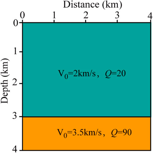
FIGURE 3. Model parameters for the two-layer models.

We run simulations for three different cases. In the first case, the fractional Laplacians in Eq. 1 are calculated by the pointwise strategy (the reference solution). In the second case, the fractional Laplacians are calculated by using the average Q value scheme (the average Q-compensated scheme). The third case is implemented by solving Eq. 11 (the proposed constant-order compensated method). The reference solution, average Q-compensated, and constant-order compensated schemes are shown in Figures 4A–C. The difference between the reference solution and the average Q-compensated is shown in Figure 4D, and the difference between the reference solution and the constant-order compensated schemes is shown in Figure 4E. Note that the color scales are the same for all snapshots. Compared to Figure 4D, the smaller residual in Figure 4E confirms the accuracy of the proposed method for sharp Q media.

FIGURE 4

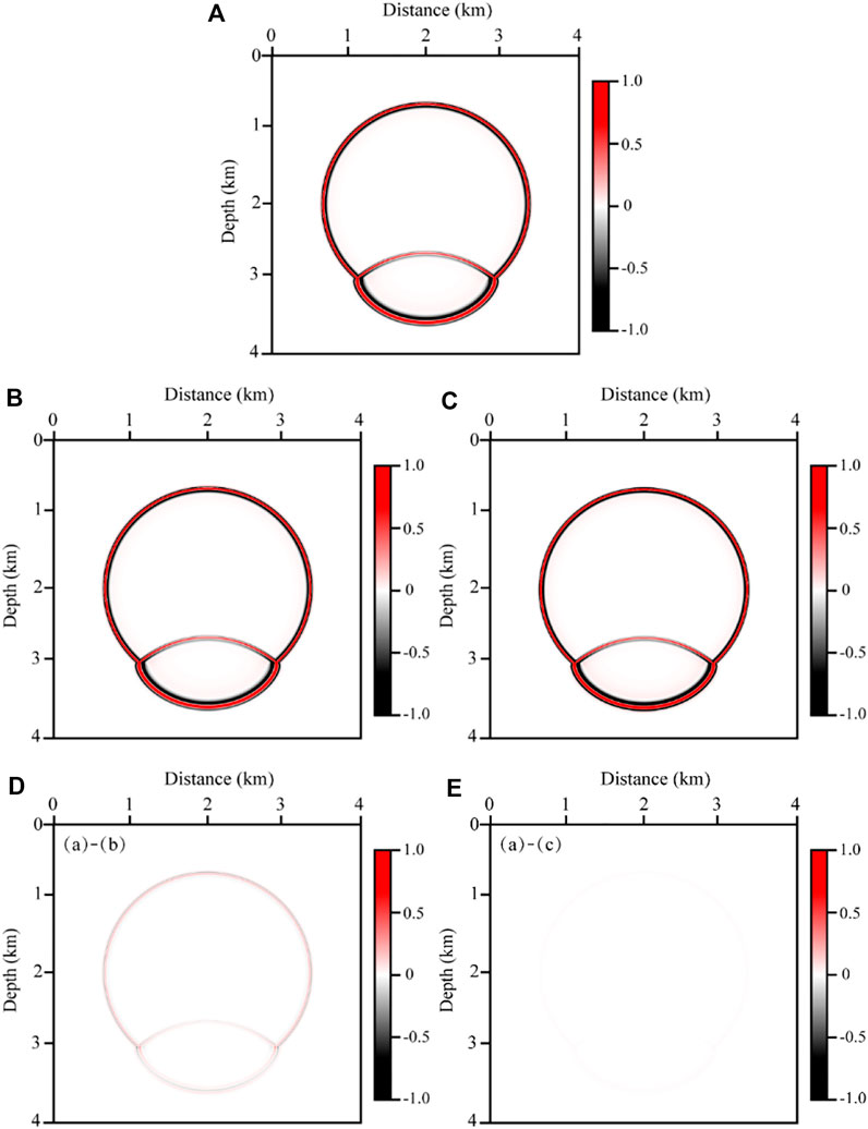
FIGURE 4. Wavefield snapshots at 700 ms for the two-layer models. (A) the reference solution, (B) the average Q scheme. (C) the constant-order scheme (D) the difference between the reference solution and average Q scheme (E) the difference between the reference solution and constant-order scheme.

Marmousi model

Furthermore, we use the Marmousi model to validate the stability and reliability of the proposed scheme in a strongly heterogeneous Q model. The velocity and Q models that are discretized into 400 × 200 points with 10 m spacing are shown in Figures 5A, B. A Ricker wavelet with a peak frequency of 25 Hz is selected as the point source. The simulation time is 2.5 s with a time step of 1 ms. Forty shots and two hundred receivers are evenly distributed at a depth of 20 m. The compensated parameter $\beta =6$ and $\sigma =0.5c_0^{2\gamma -1}{\omega }_0^{-2\gamma }\sin \left(\pi \gamma \right){\left|{\mathrm{k}}_{ref}\right|}^{2\gamma +1-\beta }$.

FIGURE 5

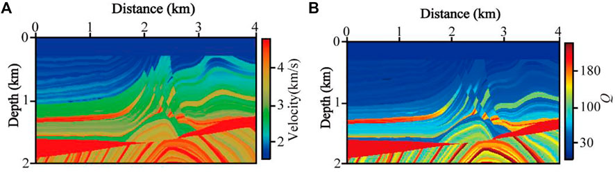
FIGURE 5. Marmousi (A) velocity and (B) Q model.

The observed shots with and without the Q attenuation are shown in Figure 6 where the first row corresponds to the elastic media and the second row correspond to the loss media. Columns 1–4 represent to the 10th, 30th, 50th, and 70th shots, respectively. All common-gathers are displayed at the same color scales. As expected, the deep structural energy in loss medium is obviously weakened due to the existence of attenuation. Figure 7 shows the migration profiles with different methods. All profiles are displayed at the same color scales. We tested four different imaging methods: the acoustic RTM to acoustic data (reference solution, Figure 7A), the acoustic RTM to viscoacoustic data (non-compensated RTM, Figure 7B), the average Q-compensated RTM (Figure 7C), and the proposed constant-order compensated RTM (our method, Figure 7D). Obviously, significant amplitude reduction (particularly for deep structures) is observed (Figure 7B) because of the attenuation property of the medium. Two compensation methods improve the imaging results without numerical instability. Although both compensation results show clear anticlinal structures because of the enhanced high-frequency components, there is still some difference between the average Q-compensated RTM and the reference solution. In contrast, Figure 7D is very similar to the reference solution.

FIGURE 6

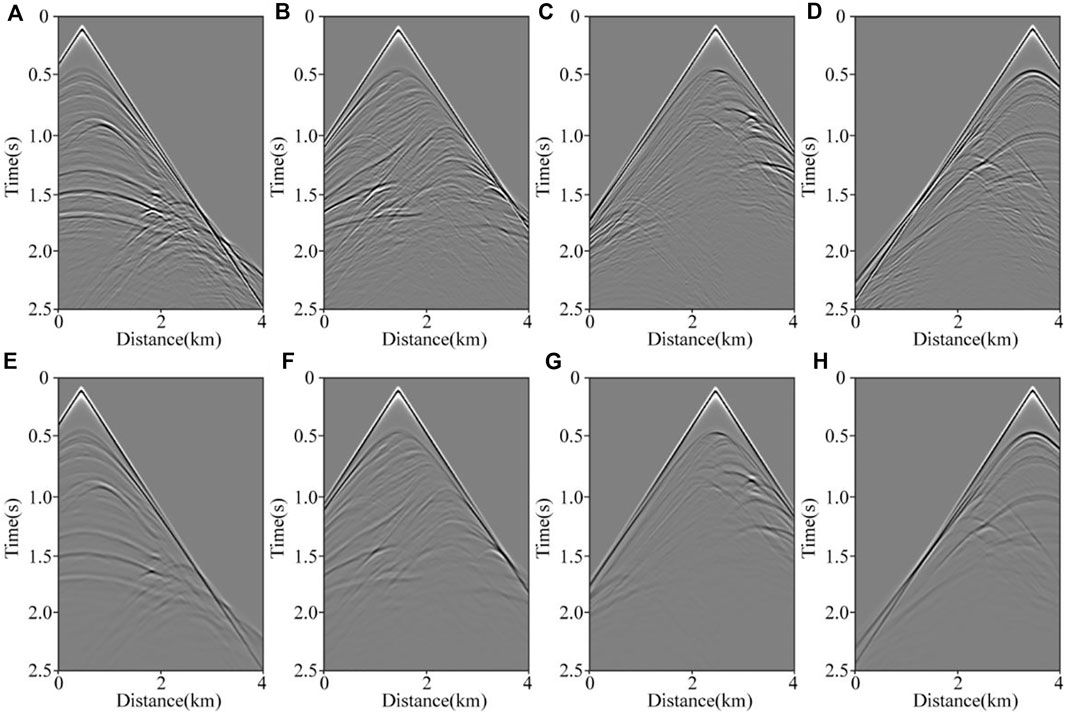
FIGURE 6. Common-gathers. The first row corresponds to the elastic media and the second row correspond to the loss media. Columns 1–4 represent to the 10th, 30th, 50th, and 70th shots, respectively.

FIGURE 7

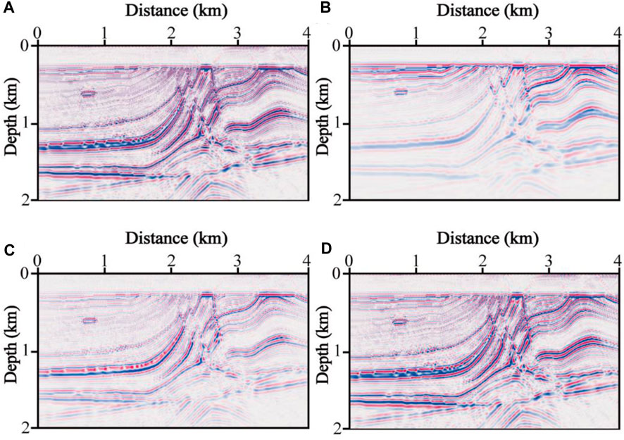
FIGURE 7. Migration results of the Marmousi model. (A) acoustic RTM to acoustic data; (B) acoustic RTM to viscoacoustic data; (C) average Q-compensated RTM; (D) constant-order compensated RTM.

We also test the possible effects of $\sigma$ on Q-RTM results in the Marmousi example and show results with the different $\sigma$ in Figure 8. We set $\text{ref}=c_0^{2\gamma -1}{\omega }_0^{-2\gamma }\sin \left(\pi \gamma \right){\left|{\mathrm{k}}_{ref}\right|}^{2\gamma +1-\beta }$ and test four different parameters, where 8a-8d represent to $\sigma =0.1\text{ref}$ (very small), $\sigma =0.5\text{ref}$; $\sigma =\text{ref}$,; $\sigma =10\text{ref}$ (very large), respectively. Migration results with the very small $\sigma$ has numerical instability (Figure 8A) and migration results with the very large $\sigma$ damages too much high-frequency information (Figure 8D). Figures 8B, C show better imaging results. Hence, it means that the more high-wavenumber signal is eliminated with $\sigma$ increases.

FIGURE 8

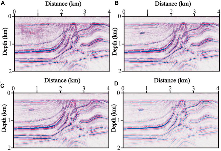
FIGURE 8. Migration results of the Marmousi model with different $\sigma$. (A) $\sigma =0.1\text{ref}$; (B) $\sigma =0.5\text{ref}$; (C) $\sigma =\text{ref}$; (D) $\sigma =10\text{ref}$.

For comparison, Figures 9A, B show vertical profiles at 1.5 km and 3.5 km along the horizontal direction, respectively. The black line, blue dashed line and red dashed line represent the reference solution, average Q-compensated, and constant-order compensated RTM, respectively. The blue dashed line suffers from amplitude mismatch and phase distortion phenomenon, while the red dashed line matches the reference trace better (particularly for deep reflections). Figure 10 represents the corresponding amplitude spectra. Compared with the non-compensated RTM (green line), the high-wavenumber components of the average Q-compensated RTM (blue dash line) and the constant-order compensated RTM (red line) are significantly improved. Furthermore, confirming the superiority of the proposed method in a strongly heterogeneous Q model, the consistency between the red and black lines is slightly better than that between the blue and black lines.

FIGURE 9

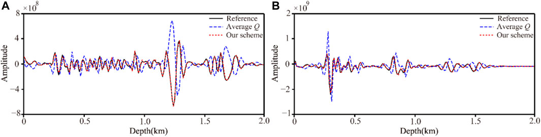
FIGURE 9. Vertical profiles of different migration images. (A) at x = 1.5 km; (B) at x = 3.5 km.

FIGURE 10

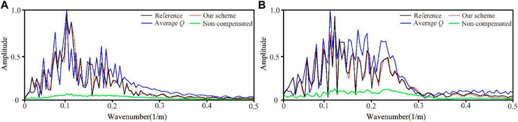
FIGURE 10. Amplitude spectra corresponding to the migrated seismic traces (A) at x = 1.5 km; (B) at x = 3.5 km.

3D overthrust model

We verify the applicability of the proposed method in the 3D case. The velocity and Q models are shown in Figures 11A, B, respectively. The model contains 550 × 200 × 150 cells with unified spatial intervals of 10 m. A total of 270 shots and 22,500 receivers are evenly located. We simulate records using a Ricker wavelet with a peak frequency of 20 Hz. The records have a duration of 2 s with a time interval of 1 ms, and the compensated parameter $\beta$ is 8.

FIGURE 11

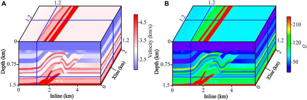
FIGURE 11. 3D overthrust model. (A) Velocity; (B) Q.

We set a maximum stacking aperture of 1.5 km for each shot to eliminate the diffraction artifacts from the long offset. Different migrated images with acoustic RTM to acoustic data (reference solution), acoustic RTM to viscoacoustic data (non-compensated), average Q-compensated RTM, and constant-order compensated RTM are shown in Figures 12A–D. Unsatisfactory imaging results, particularly below the high dip normal fault, indicate that attenuation has a certain impact on 3D migrated images, as shown in Figure 12B. Compared with Figures 12C, D agrees well with the reference solution. We extract the migrated seismic traces (x = 1,200 m, y = 1,200 m) shown in Figure 13, where the black line, blue dashed line and red dashed line represent the reference solution, average Q-compensated, and constant-order compensated RTM, respectively. The blue line has a shifted phase due to inaccurate attenuation compensation, affecting the precise identification of the target layer and horizon interpretation. In contrast, the red line maintains polarity consistency with the reference solution, demonstrating the effectiveness of the proposed method in the 3D case.

FIGURE 12

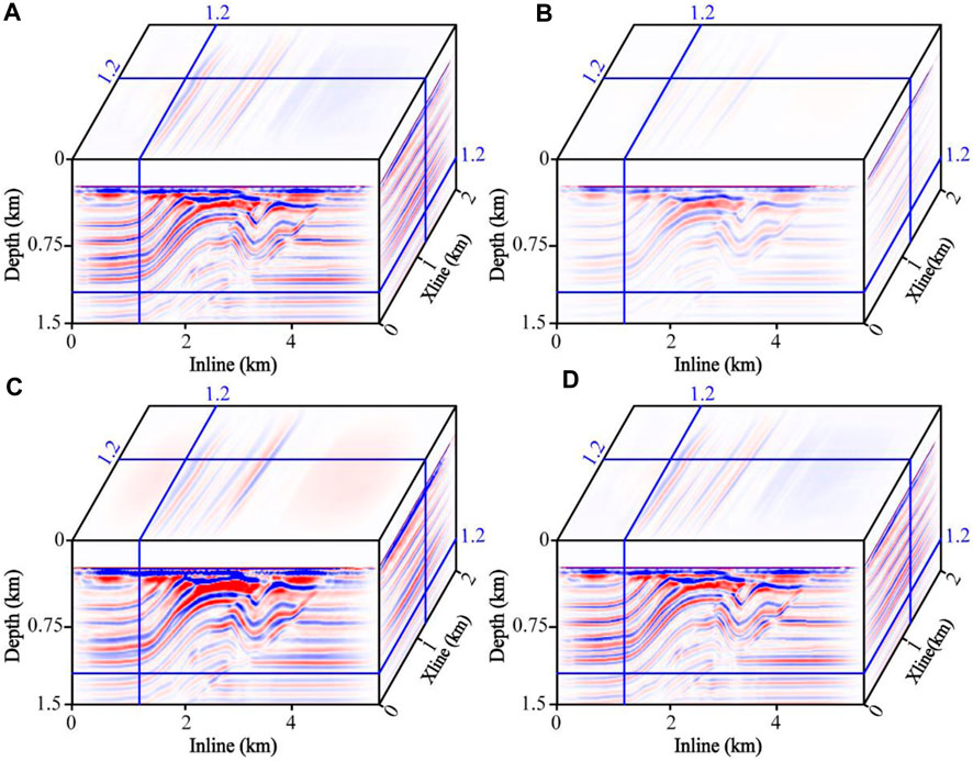
FIGURE 12. Migrated images of 3D overthrust model. (A) acoustic RTM to acoustic data; (B) acoustic RTM to viscoacoustic data; (C) average Q-compensated RTM; (D) constant-order compensated RTM.

FIGURE 13

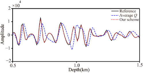
FIGURE 13. The traces selected at (x = 1,200 m, y = 1,200 m).

Field data from a land survey

To confirm the potential of our approach in field applications, we apply the proposed constant-order compensated RTM to the field data from a land survey. The velocity (Sava and Vlad, 2008) and Q models (Tonn, 1991) are shown in Figures 14A, B, respectively. The model has 900 × 300 cells with a grid size of 20 m² × 20 m². The maximum and minimum velocities are 5,515 and 2,213 m/s, respectively.

FIGURE 14

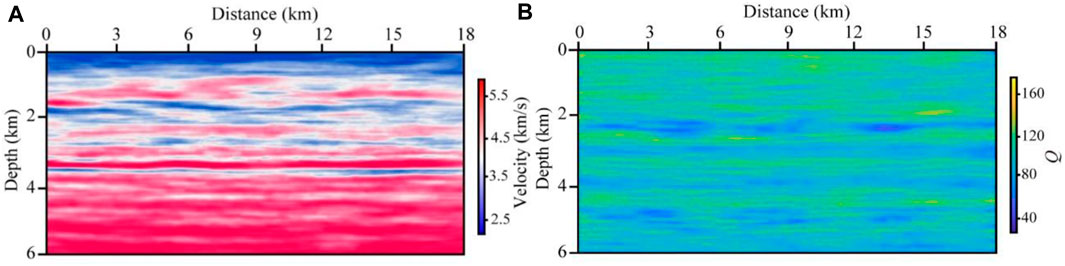
FIGURE 14. (A) Velocity model; (B) Q model.

The record duration is 5 s, with a time step of 1 ms. A 2D acquisition line contains 240 excitation sources. We set the maximum stacking aperture of 3.0 km for each shot to eliminate the diffraction artifacts from the long offset, and the compensated parameter $\beta$ is 6. Figures 15A–D show the common-shot gathers of 50, 100, 150, and 200. All the shots were preprocessed, including static correction, surface wave attenuation, multiple attenuations, and bandpass filtering.

FIGURE 15

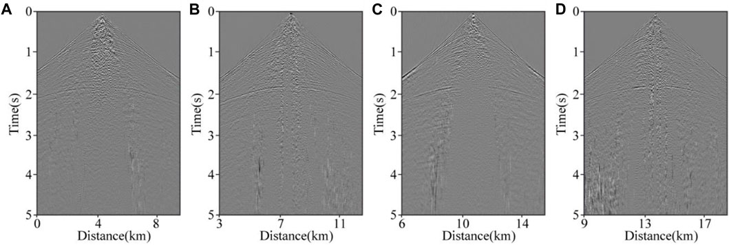
FIGURE 15. Shot-gathers of field data. (A) the 50th shot; (B) the 100th shot; (C) the 150th shot; (D) the 200th shot.

The acoustic RTM (non-compensated) and the constant-order compensated RTM are shown in Figures 16A, B. Compared to the acoustic RTM results (Figure 16A), the proposed compensated RTM (Figure 16B) shows a higher resolution and has better illumination of the deep reflections. Specifically, compared with Figure 16B, the continuity of the structures in Figure 16A is destroyed, and the lateral variation in the reflectors is worse (approximately 2 km depth denoted by the red arrow) since acoustic RTM ignores the attenuation compensation. This can be considered a fake fault, thus degrading the reliability of the interpretation. A zoomed-in section of the red box in Figure 16 is shown in Figure 17, with Figures 17A, B showing the acoustic and the constant-order compensated RTM, respectively. The reflections of Figure 17B are stronger than Figure 17A. The wavenumber spectra of the images at x = 5 and 9 km are shown in Figures 18A, B, respectively. Indicating that the proposed method can effectively recover the amplitude, the wavenumber components are increased visibly after Q compensation (Figure 18).

FIGURE 16

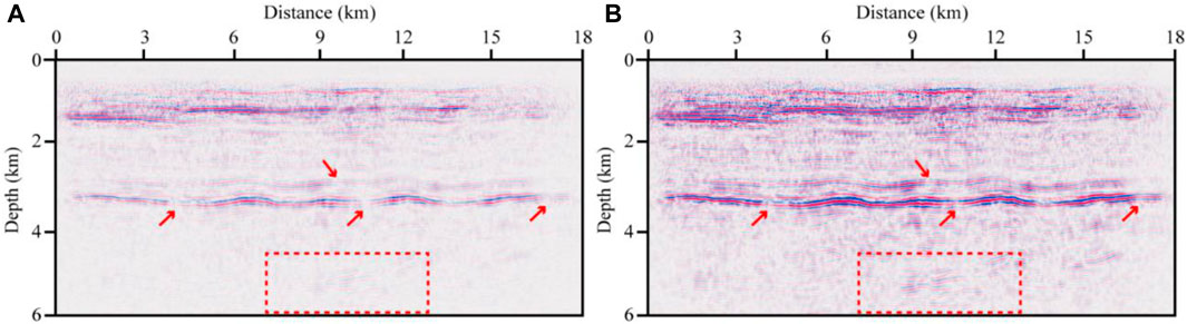
FIGURE 16. Migrated images of the field data. (A) acoustic RTM; (B) constant-order compensated RTM.

FIGURE 17

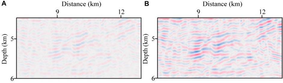
FIGURE 17. Zoom-in of the migrated image (A) acoustic RTM (B) constant-order compensated RTM.

FIGURE 18

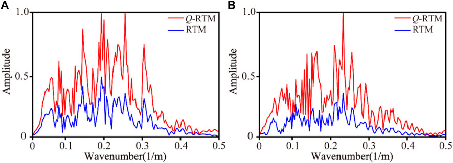
FIGURE 18. Amplitude spectra corresponding to the migrated seismic traces (A) at x = 5 km; (B) at x = 9 km.

Discussion

The accuracy of migration imaging is essential for seismic data processing and structural interpretation, and calculation efficiency is the premise of industrial practicality. Here, we discuss the cost of several compensation schemes and their precision of imaging results. The numerical examples are implemented using the Compute Unified Device Architecture programming on an Nvidia Geforce RTX 2080Ti. We run simulations for three different cases: the exact solution, the average Q-compensated method, and the constant-order compensated scheme. In Table 1, we list the computation time with the different methods for the 2D Marmousi and 3D overthrust models. For quantitative comparison, we calculate the mean relative absolute error and mark them on the right side of Table 1. The model parameters are consistent with the previous test. Due to the huge amount of computation, the exact solution (calculated by pointwise FFT) only runs a shot simulation. As shown in Table 1, even though the exact solution can accurately simulate the propagation of seismic waves, its numerical implementation is more expensive. Compared with the pointwise FFT, the average Q scheme significantly improves computing efficiency under the condition of sacrificing computational accuracy. Although the numerical implementation of the constant-order compensated schemes is slightly more expensive (about 1.3 times slower) than the average Q scheme in the 3D case, the calculation accuracy was significantly improved. As mentioned above, the computational cost and accuracy test demonstrated that the proposed method provides a better trade-off between imaging accuracy and calculation efficiency. In this paper, we do not test the 3D field data because a single GPU card cannot afford its memory requirements. Hence, the future research direction on this topic is the 3D field data Q-compensated RTM by multi-GPU computing based on model segmentation.

TABLE 1

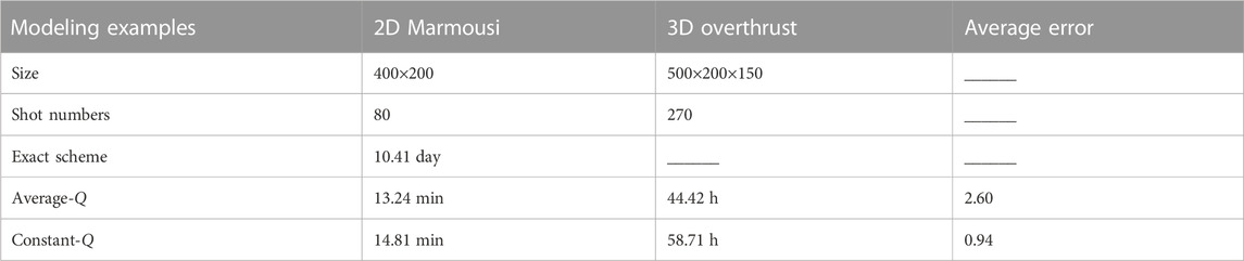
TABLE 1. Calculation-time comparison between different RTM schemes.

Conclusion

We presented a stabilized Q-compensated RTM scheme which has the explicit stabilization terms in the time-space domain. The proposed Q-compensated RTM avoids the compensating error introduced by averaging spatially varying fractional orders, and it enables us to precisely compensate for the seismic attenuation in complex heterogeneous Q media. The proposed algorithm enhances the resolution in Q-RTM without significantly increasing computational cost. The explicit stabilization term is free from frequent Fourier transforms, so it is expected to simplify the Q-RTM workflow. Numerical simulation examples for homogeneous models demonstrated that the numerical solutions of the proposed wave equation agree with those of the original viscoacoustic wave equation. Furthermore, the synthetic and land field datasets demonstrate the superiority and effectiveness of the proposed approach. We anticipate that the proposed Q-compensated RTM will directly benefit imaging applications as well as enhance the reliability of seismic interpretations.

Data availability statement

The original contributions presented in the study are included in the article/supplementary material, further inquiries can be directed to the corresponding author.

Author contributions

SL, methodology, formal analysis, visualization, writing—original draft. YS, investigation, visualization: supervision, conceptualization. NW, writing—review and editing. WW, software. LS, writing—review and editing. YW, formal analysis.

Funding

This work is partly supported by the National Natural Science Foundation of China (41930431, 42274171, 42204129), the Joint Guiding Project of the Natural Science Foundation of Heilongjiang Province (LH 2021D009).

Conflict of interest

The authors declare that the research was conducted in the absence of any commercial or financial relationships that could be construed as a potential conflict of interest.

Publisher’s note

All claims expressed in this article are solely those of the authors and do not necessarily represent those of their affiliated organizations, or those of the publisher, the editors and the reviewers. Any product that may be evaluated in this article, or claim that may be made by its manufacturer, is not guaranteed or endorsed by the publisher.

References

Aki, K., and Richards, P. (1980). Quantitative seismology. Concord, Canada: Freeman Publication Co.

Google Scholar

Bai, T., Zhu, T., and Tsvankin, I. (2019). Attenuation compensation for time-reversal imaging in VTI media. Geophysics 84 (4), C205–C216. doi:10.1190/geo2018-0532.1

CrossRef Full Text | Google Scholar

Bickel, S. H., and Natarajan, R. (1985). Plane-wave Q deconvolution. Geophysics 50 (9), 1426–1439. doi:10.1190/1.1442011

CrossRef Full Text | Google Scholar

Carcione, J. M. (2008). Theory and modeling of constant-Q P-and S-waves using fractional time derivatives. Geophysics 74 (1), T1–T11. doi:10.1190/1.3008548

CrossRef Full Text | Google Scholar

Carcione, J. M. (1990). Wave propagation in anisotropic linear viscoelastic media: Theory and simulated wavefields. Geophys. J. R. Astronomical Soc. 101 (3), 739–750. doi:10.1111/j.1365-246X.1990.tb05580.x

CrossRef Full Text | Google Scholar

Causse, E., and Ursin, B. (2000). Viscoacoustic reverse-time migration. J. Seismic Explor. 9 (2), 165–184.

Google Scholar

Chen, H., Zhou, H., Li, Q., and Wang, Y. (2016). Two efficient modeling schemes for fractional Laplacian viscoacoustic wave equation. Geophysics 81 (5), T233–T249. doi:10.1190/GEO2015-0660.1

CrossRef Full Text | Google Scholar

Chen, H., Zhou, H., and Rao, Y. (2020a). An implicit stabilization strategy for Q-compensated reverse time migration. Geophysics 85 (3), S169–S183. doi:10.1190/geo2019-0235.1

CrossRef Full Text | Google Scholar

Chen, H., Zhou, H., and Rao, Y. (2020c). Source wavefield reconstruction in fractional laplacian viscoacoustic wave equation-based full waveform inversion. IEEE Trans. Geoscience Remote Sens. 59 (8), 6496–6509. doi:10.1109/TGRS.2020.3029630

CrossRef Full Text | Google Scholar

Chen, H., Zhou, H., and Tian, Y. (2020b). Least-squares reverse-time migration based on a fractional Laplacian viscoacoustic wave equation. Oil Geophys. Prospect. 55 (3), 616–626.

Google Scholar

Claerbout, Jon F. (1971). Toward a unified theory of reflector mapping. Geophysics 36 (3), 467–481. doi:10.1190/1.1440185

CrossRef Full Text | Google Scholar

Dai, N., and West, G. F. (1994). Inverse Q migration: 64th annual international meeting. Tulsa, Oklahoma: Society of Exploration Geophysicists, 1418–1421. doi:10.1190/1.1822799

CrossRef Full Text | Google Scholar

Dasgupta, R., and Roger, A. (1998). Estimation of Q from surface seismic reflection data. Geophysics 63 (6), 2120–2128. doi:10.1190/1.1444505

CrossRef Full Text | Google Scholar

Deng, F., and McMechan, G. A. (2008). Viscoelastic true-amplitude prestack reverse-time depth migration. Geophysics 73 (4), S143–S155. doi:10.1190/1.2938083

CrossRef Full Text | Google Scholar

Dutta, G., and Schuster, G. (2014). Attenuation compensation for leastsquares reverse time migration using the viscoacoustic-wave equation. Geophysics 79 (6), S251–S262. doi:10.1190/geo2013-0414.1

CrossRef Full Text | Google Scholar

Dvorkin, J. P., and Mavko, G. (2006). Modeling attenuation in reservoir and nonreservoir rock. Lead. Edge 25 (2), 194–197. doi:10.1190/1.2172312

CrossRef Full Text | Google Scholar

Futterman, W. I. (1962). Dispersive body waves. J. Geophys. Res. 67, 5279–5291. doi:10.1029/JZ067i013p05279

CrossRef Full Text | Google Scholar

Guo, P., McMechan, G., and Guan, H. (2016). Comparison of two viscoacoustic propagators for Q-compensated reverse time migration. Geophysics 81 (5), S281–S297. doi:10.1190/geo2015-0557.1

CrossRef Full Text | Google Scholar

Guo, P., and McMechan, G. (2015). Separation of absorption and dispersion effects in Q-compensated viscoelastic RTM. Proceedings of the 85th Annual International Meeting, SEG, Expanded 507 Abstracts, 3966–3971, New Orleans, Louisiana. October 2015. doi:10.1190/segam2015-5824203.1

CrossRef Full Text | Google Scholar

Hargreaves, N. D., and Calvert, A. J. (1991). Inverse Q filtering by Fourier transform. Geophysics 56 (4), 519–527. doi:10.1190/1.1443067

CrossRef Full Text | Google Scholar

Kjartansson, E. (1979). Constant Q-wave propagation and attenuation. J. Geophys. Res. Solid Earth 84 (9), 4737–4748. doi:10.1029/JB084iB09p04737

CrossRef Full Text | Google Scholar

Kolsky, H. (1956). Taylor & francis online: LXXI. The propagation of stress pulses in viscoelastic solids. Philos. Mag. 1 (8), 693–710. doi:10.1080/14786435608238144

CrossRef Full Text | Google Scholar

Korneev, V. A., Goloshubin, G. M., Daley, T. M., and Silinet, D. B. (2004). Seismic low-frequency effects in monitoring fluid-saturated reservoirs. Geophysics 69 (2), 522–532. doi:10.1190/1.1707072

CrossRef Full Text | Google Scholar

Li, Q., Zhou, H., Zhang, Q., Chen, H., and Sheng, S. (2016b). Efficient reverse time migration based on fractional Laplacian viscoacoustic wave equation. Geophys. J. Int. 204 (1), 488–504. doi:10.1093/gji/ggv456

CrossRef Full Text | Google Scholar

Liu, H., and Luo, Y. (2021). An analytic signal-based accurate time-domain viscoacoustic wave equation from the constant-Q theory. Geophysics 86 (3), T117–T126. doi:10.1190/geo2020-0154.1

CrossRef Full Text | Google Scholar

Mainardi, F. (2010). Fractional calculus and waves in linear viscoelasticity: An introduction to mathematical models. Singapore: World Scientific.

Google Scholar

Margrave, G., Lamoureux, M., and Henley, D. (2011). Gabor deconvolution: Estimating reflectivity by nonstationary deconvolution of seismic data. Geophysics 76 (3), W15–W30. doi:10.1190/1.3560167

CrossRef Full Text | Google Scholar

McDonal, F. J., Angona, F. A., Mills, R. L., Sengbush, R. L., Van Nostrand, R. G., and White, J. E. (1958). Attenuation of shear and compressional waves in Pierre shale. Geophysics 23 (3), 421–439. doi:10.1190/1.1438489

CrossRef Full Text | Google Scholar

Mittet, R. (2007). A simple design procedure for depth extrapolation operators that compensate for absorption and dispersion. Geophysics 72 (2), S105–S112. doi:10.1190/1.2431637

CrossRef Full Text | Google Scholar

Mu, X., Huang, J., Yang, J., Li, Z., and Ivan, M. S. (2021). Viscoelastic wave propagation simulation using new spatial variable-order fractional Laplacians. Bull. Seismol. Soc. Am. 112 (1), 48–77. doi:10.1785/0120210099

CrossRef Full Text | Google Scholar

Ren, Z., Bao, Q., and Xu, S. (2022). Memory-efficient source wavefield reconstruction and its application to 3D reverse time migration. Geophysics 87 (1), S21–S34. doi:10.1190/geo2020-0580.1

CrossRef Full Text | Google Scholar

Rossikhin, Y. A., and Shitikova, M. V. (2010). Application of fractional calculus for dynamic problems of solid mechanics: Novel trends and recent results. Appl. Mech. Rev. 63 (1), 010801. doi:10.1115/1.4000563

CrossRef Full Text | Google Scholar

Sava, P., and Vlad, I. (2008). Numeric implementation of wave-equation migration velocity analysis operators. Geophysics 73 (5), VE145–VE159. doi:10.1190/1.2953337

CrossRef Full Text | Google Scholar

Sun, J., Zhu, T., and Fomel, S. (2015). Viscoacoustic modeling and imaging using low-rank approximation. Geophysics 80 (5), A103–A108. doi:10.1190/geo2015-0083.1

CrossRef Full Text | Google Scholar

Sun, J., and Zhu, T. (2018). Strategies for stable attenuation compensation in reverse-time migration. Geophys. Prospect. 66 (3), 498–511. doi:10.1111/1365-2478.12579

CrossRef Full Text | Google Scholar

Tonn, R. (1991). The determination of the seismic quality factor Q from VSP data: A comparison of different computational methods. Geophys. Prospect. 39 (1), 1–27. doi:10.1111/j.1365-2478.1991.tb00298.x

CrossRef Full Text | Google Scholar

Tselentis, G. A. (1998). Intrinsic and scattering seismic attenuation in W. Greece. Pure Appl. Geophys. 153 (2), 703–712. doi:10.1007/s000240050215

CrossRef Full Text | Google Scholar

Wang, N., Xing, G., Zhu, T., Zhou, H., and Shi, Y. (2022). Propagating seismic waves in VTI attenuating media using fractional viscoelastic wave equation. J. Geophys. Res. Solid Earth 127, e2021JB023280. doi:10.1029/2021JB023280

CrossRef Full Text | Google Scholar

Wang, N., Yang, D., and Liu, F. (2012). Weak dispersion wave-field simulations: A predictor-corrector algorithm for solving acoustic and elastic wave equations. J. Seismic Explor. 21 (2), 125–152.

Google Scholar

Wang, N., Zhou, H., Chen, H., Xia, M., Wang, S., Fang, J., et al. (2018a). A constant fractional-order viscoelastic wave equation and its numerical simulation scheme. Geophysics 83 (1), T39–T48. doi:10.1190/geo2016-0609.1

CrossRef Full Text | Google Scholar

Wang, N., Zhu, T., Zhou, H., Chen, H., Zhao, X., and Tian, Y. (2020). Fractional Laplacians viscoacoustic wavefield modeling with k-space-based time-stepping error compensating scheme. Geophysics 85 (1), T1–T13. doi:10.1190/geo2019-0151.1

CrossRef Full Text | Google Scholar

Wang, Y. (2002). A stable and efficient approach of inverse Q filtering. Geophysics 67 (2), 657–663. doi:10.1190/1.1468627

CrossRef Full Text | Google Scholar

Wang, Y., and Guo, J. (2004). Seismic migration with inverse Q filtering. Geophys. Res. Lett. 31 (21), 163–183. doi:10.1029/2004GL020525

CrossRef Full Text | Google Scholar

Wang, Y., Harris, J. M., Bai, M., Saad, O. M., Yang, L., and Chen, Y. (2021). An explicit stabilization scheme for Q-compensated reverse time migration. Geophysics 87 (3), F25–F40. doi:10.1190/geo2021-0134.1

CrossRef Full Text | Google Scholar

Wang, Y., Li, D. Z., and Harris, J. M. (2019). A generalized stabilization scheme for seismic Q compensation. SEG Technical Program Expanded Abstracts: 4251–4255, September 2019, San Antonio, Texas, USA. doi:10.1190/segam2019-3198472.1

CrossRef Full Text | Google Scholar

Wang, Y. (2003). Quantifying the effectiveness of stabilized inverse Q filtering. Geophysics 68 (1), 337–345. doi:10.1190/1.1543219

CrossRef Full Text | Google Scholar

Wang, Y., Zhou, H., Chen, H., and Chen, Y. (2017). Adaptive stabilization for q-compensated reverse time migration. Geophysics 83 (1), S15–S32. doi:10.1190/geo2017-0244.1

CrossRef Full Text | Google Scholar

Wang, Y., Zhou, H., Zhao, X., Zhang, Q., Zhao, P., Yu, X., et al. (2018b). CuQ-RTM: A CUDA-based code package for stable and efficient Q-compensated reverse time migration. Geophysics 84 (1), 1JF–Z5. doi:10.1190/geo2017-0624.1

CrossRef Full Text | Google Scholar

Xie, Y., Sun, J., Zhang, Y., and Zhou, J. (2015). Compensating for visco-acoustic effects in TTI reverse time migration. Proceedings of the 85th Annual International Meeting, SEG, expanded abstracts, New Orleans, Louisiana, October 2015, pp 3996–4001.

CrossRef Full Text | Google Scholar

Xing, G., and Zhu, T. (2020). A viscoelastic model for seismic attenuation using fractal mechanical networks. Geophys. J. Int. 224 (3), 1658–1669. doi:10.1093/gji/ggaa549

CrossRef Full Text | Google Scholar

Xing, G., and Zhu, T. (2021). Decoupled Fréchet kernels based on a fractional viscoacoustic wave equation. Geophysics 87 (1), T61–T70. doi:10.1190/geo2021-0248.1

CrossRef Full Text | Google Scholar

Xing, G., and Zhu, T. (2019). Modeling frequency-independent Q viscoacoustic wave propagation in heterogeneous media. J. Geophys. Res. Solid Earth 124 (11), 11568–11584. doi:10.1029/2019JB017985

CrossRef Full Text | Google Scholar

Xu, T., and McMechan, G. (1995). Composite memory variables for viscoelastic synthetic seismograms. Geophys. J. Int. 121 (2), 634–639. doi:10.1111/j.1365-246X.1995.tb05738.x

CrossRef Full Text | Google Scholar

Xue, Z., Sun, J., Fomel, S., and Zhu, T. (2017). Accelerating full-waveform inversion with attenuation compensation. Geophysics 83 (1), A13–A20. doi:10.1190/geo2017-0469.1

CrossRef Full Text | Google Scholar

Yang, J., and Zhu, H. (2018a). A time-domain complex-valued wave equation for modelling visco-acoustic wave propagation. Geophys. J. Int. 215 (2), 1064–1079. doi:10.1093/gji/ggy323

CrossRef Full Text | Google Scholar

Yang, J., and Zhu, H. (2018b). Viscoacoustic reverse-time migration using a time-domain complex-valued wave equation. Geophysics 83 (6), S505–S519. doi:10.1190/geo2018-0050.1

CrossRef Full Text | Google Scholar

Yang, J., Huang, J., Zhu, H., and Dai, N. (2021). Viscoacoustic reverse-time migration with a robust space-wavenumber domain attenuation compensation operator. Geophysics 86 (5), S339–S353. doi:10.1190/geo2020-0608.1

CrossRef Full Text | Google Scholar

Yang, R., Mao, W., and Chang, X. (2015). An efficient seismic modeling in viscoelastic isotropic media. Geophysics 80 (1), T63–T81. doi:10.1190/geo2013-0439.1

CrossRef Full Text | Google Scholar

Yao, J., Zhu, T., Hussain, F., and Kouri, D. J. (2016). Locally solving fractional Laplacian viscoacoustic wave equation using Hermite distributed approximating functional method. Geophysics 82 (2), T59–T67. doi:10.1190/geo2016-0269.1

CrossRef Full Text | Google Scholar

Yilmaz, O. (2001). Seismic data analysis. SEG. Tulsa.

Google Scholar

Zhang, W., and Gao, J. (2022). Attenuation compensation for wavefield-separation-based least-squares reverse time migration in viscoelastic media. Geophys. Prospect. 70 (2), 280–317. doi:10.1111/1365-2478.13161

CrossRef Full Text | Google Scholar

Zhang, W., Gao, J., Cheng, Y., Su, C., Liang, H., and Zhu, J. (2022). 3D image-domain least-squares reverse time migration with L1 norm constraint and total variation regularization. IEEE Trans. Geoscience Remote Sens. 60, 1–14. doi:10.1109/TGRS.2022.3196428

CrossRef Full Text | Google Scholar

Zhang, W., and Gao, J. (2021). Deep-learning full-waveform inversion using seismic migration images. IEEE Trans. Geoscience Remote Sens. 60, 1–18. doi:10.1109/TGRS.2021.3062688

CrossRef Full Text | Google Scholar

Zhang, Y., Zhang, P., and Zhang, H. (2010). Compensating for visco-acoustic effects in reverse-time migration. Seg. Tech. Program Expand. Abstr. 3160–3164. doi:10.1190/1.3513503

CrossRef Full Text | Google Scholar

Zhao, X. H., Zhou, Y., Wang, H., Chen, H., Zhou, Z., Sun, P., et al. (2018b). A stable approach for Q-compensated viscoelastic reverse time migration using excitation amplitude imaging condition. Geophysics 83 (5), S459–S476. doi:10.1190/geo2018-0222.1

CrossRef Full Text | Google Scholar

Zhao, Y., Mao, N., and Ren, Z. (2018a). A stable and efficient approach of Q reverse time migration. Geophysics 83 (6), S557–S567. doi:10.1190/geo2018-0022.1

CrossRef Full Text | Google Scholar

Zhu, T., and Bai, T. (2018). Efficient modeling of wave propagation in a vertical transversely isotropic attenuative medium based on fractional Laplacian. Geophysics 84 (3), T121–T131. doi:10.1190/geo2018-0538.1

CrossRef Full Text | Google Scholar

Zhu, T., Harris, J. M., and Biondi, B. (2014). Q-compensated reverse-time migration. Geophysics 79 (3), S77–S87. doi:10.1190/geo2013-0344.1

CrossRef Full Text | Google Scholar

Zhu, T., and Harris, J. M. (2014). Modeling acoustic wave propagation in heterogeneous attenuating media using decoupled fractional Laplacians. Geophysics 79 (3), T105–T116. doi:10.1190/geo2013-0245.1

CrossRef Full Text | Google Scholar

Zhu, T. (2016). Implementation aspects of attenuation compensation in reverse-time migration. Geophys. Prospect. 64 (3), 657–670. doi:10.1111/1365-2478.12301

CrossRef Full Text | Google Scholar

Zhu, T. (2017). Numerical simulation of seismic wave propagation in viscoelastic-anisotropic media using frequency-independent Q wave equation. Geophysics 82 (4), 1–WA10. doi:10.1190/geo2016-0635.1

CrossRef Full Text | Google Scholar

Zhu, T., and Sun, J. (2017). Viscoelastic reverse time migration with attenuation compensation. Geophysics 82 (2), S61–S73. doi:10.1190/geo2016-0239.1

CrossRef Full Text | Google Scholar

Zhu, T. Y., Carcione, J. M., and Harris, J. M. (2013). Approximating constant-Q seismic propagation in the time domain. Geophys. Prospect. 61 (5), 931–940. doi:10.1111/1365-2478.12044

CrossRef Full Text | Google Scholar