 Christoffer Karoff1,2,3*
 Angel Liduvino Vara-Vela1,2,3
- 1Department of Geoscience, Aarhus University, Aarhus, Denmark
- 2Department of Physics and Astronomy, Aarhus University, Aarhus, Denmark
- 3iCLIMATE Aarhus University Interdisciplinary Centre for Climate Change, Aarhus, Denmark
Over the last decade we have witnessed a rapid, so far unexplained, increase in the emission of methane to the atmosphere and this increase could lead to an acceleration of the ongoing climate changes. The increase is likely to originate from agriculture, but oil and gas production as well as wetlands are also under suspicion. The best way to quantify the emission of methane and other greenhouse gasses to our atmosphere is by using space based remote sensing. Here, we analyse 3 years of measurements of the column-averaged dry-air mole fraction of methane from the Tropospheric Monitoring Instrument on Sentinel-5P obtained with two different retrieval methods in order to evaluate the dependency on geographic, land cover type and season. The land cover types were obtained from the Moderate Resolution Imaging Spectroradiometer aboard the Terra and Aqua satellites and from the World Cover data product using observations from the Copernicus Sentinel-1 and Sentinel-2 missions. The analysis reveals that while the highest methane concentrations are generally found over croplands, the lowest are generally found over shrublands, which is in agreement with expectations. It is more surprising that the analysis also reveals lower than average methane concentrations over wetlands as wetlands are generally thought to be a major source of methane emission. Until this discrepancy is resolved the methane concentration over wetlands from the Tropospheric Monitoring Instrument on Sentinel-5P should be handled with caution. It is also found that the annual methane cycle, as seen in the measured methane concentrations, for croplands, shrublands and savannas is delayed in Africa compared to Asia.
1 Introduction
Greenhouse gasses can be monitored from satellites using infrared spectra of reflected sunlight. Such measurements hold a large potential for not only understanding greenhouse gas emission, but also for reducing greenhouse gas emission by providing objective and transparent information that can be used in the taxating of the largest emitters.
The greenhouse gasses that contribute most to global warming, except for water, are carbon dioxide (CO2) and methane (CH4) and the atmospheric concentration of both these gasses can be measured with satellites. The column-averaged dry-air mole fraction of CO2 and CH4 are denoted XCO2 and XCH4, respectively and changes in these quantities can be used to estimate the growth rates. In this way, the annual grow rates of XCO2 and XCH4 have been measured to 2.28 ± 0.04 ppm yr−1 and 7.9 ± 0.2 ppb yr−1, respectively (Reuter et al., 2020). Over the last decade we have witnessed a rapid increase in the annual growth rate of CH4 in the atmosphere (Nisbet et al., 2016; Saunois et al., 2020). An increase that largely remains unexplained (Saunois et al., 2016). One of the main reasons for this is that the uncertainties on the estimates of local emission from different land cover types is still very large – uncertainties of the order of 100% are not uncommon (see, e.g., Bloom et al., 2017).
Measurements of XCO2 and XCH4 can be used to estimate the emission of these greenhouse gasses using an inversion approach (Maasakkers et al., 2019). This is called a top-down approach and can be compared to estimates based on a bottom-up approach utilising inventories of anthropogenic emission as well as models of natural emission (Friedlingstein et al., 2020; Saunois et al., 2020). The uncertainties on both the top-down and the bottom-up approach are large and difficult to assess and the situation is further complicated by the fact that the bottom-up approach is often used as input to the top-down approached, where combinations of emission inventories are used as prior for the inversion (Maasakkers et al., 2019). There is therefore a need for data driven approaches that can test the results, uncertainties and conclusions from the top-down and the bottom-up approaches with as few assumptions as possible. One such data driven approach was presented by Buchwitz et al. (2017), who derived an analytical approach for calculating methane emission based on XCH4 as well as local pressure and wind velocity.
XCO2 and XCH4 have been measured with different precision and temporal and spatial resolution (see, e.g., Reuter et al., 2020). Current state-of-the-art is provided by the TROPOspheric Monitoring Instrument (TROPOMI) on board the Sentinel five Precursor (S5-P), which is capable of measuring XCH4 with a precision of 14.0 ppb, a resolution of 5.5 x 7 km, a revisit time of 16 days (Schneising et al., 2019). These observations have been used in different applications such as: understanding the role of wetlands in the appeared large CH4 emission from South Sudan (Pandey et al., 2021), evaluating the year-to-year anomalies in tropical wetland CH4 emission (Parker et al., 2018), analysing the effect of increased rainfall on wetland CH4 emission in East Africa (Lunt et al., 2021) and estimating CH4 from oil and gas production regions in the United Sates (Zhang et al., 2020b; de Gouw et al., 2020) and Russia (Ialongo et al., 2021). In addition, due to its high observational density and resolution, TROPOMI concentrations are being used in cloud-based facilities developed to respond to a growing demand for tools to infer regional methane emissions (Varon et al., 2022).
Here we take a data driven approach to analyse the entire TROPOMI data set that is inspired by the approach in Buchwitz et al. (2017). We use the TROPOMI data set to calculate distributions of the methane concentrations for different land cover types, different continents and different seasons. Assuming that the measurements have been corrected correctly for differences in the albedo of the different land cover types, this analysis allows to assess differences in the methane emission from different land cover types as function of continent and season. The approach is built on the large number theorem in the sense that a single measurement does not say much about the methane emission of the land cover type from which is was taken over, but 106 measurements does.
It should however, be stressed that we analyse methane concentrations and not emissions in this study. The analysis can thus not be used to evaluate the total methane emission from a given land cover type, only the relative methane emission from a parcel of a given land cover type.
2 Data and methods
2.1 Sentinel-5P observations
The TROPOMI instrument is an imaging spectrograph with 7 x 7 km2 resolution (upgraded to 5.5 x 7 km2 in August 2019). Measurements of XCH4 is produced by the operational methane retrieval algorithm (Hu et al., 2016) using a forward model where the observed spectra are matched to spectra from a radiative transfer model by varying XCH4 in an inversion procedure. The operational methane retrieval algorithm also produce measurements of XCO as a byproduct. The XCH4 measured from TROPOMI covered the period 20 December 2017 to 21 December 2020 is shown in Figure 1.
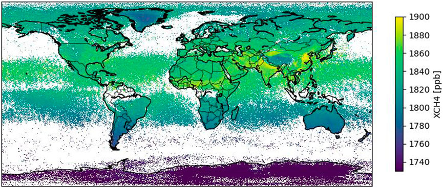
FIGURE 1. Average measurements of XCH4 covering the period 20 December 2017 to 21 December 2020 obtained with the WFM-DOAS algorithm in Schneising et al. (2019). The figure has been calculated by mapping the observations into a grid with a cell size of 0.036 times 0.072°. The well know interhemispheric gradient in XCH4 (Hu et al., 2016), with stronger values in the northern compared to the southern hemisphere is clearly visible. The largest values of XCH4 is seen over central Africa and southern Asia. Data points from high-elevated sites have been removed by the quality filter described in Schneising et al. (2019), as they are associated with large uncertainties.
2.2 TROPOMI CH4 retrieval algorithms
Schneising et al. (2019) presented an improved reduction of the uncertainty in the TROPOMI observations based on the Weighting Function Modified Differential Optical Absorption Spectroscopy (WFM-DOAS) algorithm. The WFM-DOAS algorithm is similar to the operational methane retrieval algorithm, except that it includes a machine learning based quality filter that removes measurements with high uncertainties due mainly to large solar zenith angles and a machine learning based correction of systematic errors due to underestimation of XCH4 over dark surfaces. The WFM-DOAS algorithm also uses another forward radiative transfer model compared to the operational methane retrieval algorithm that includes solar zenith angle, altitude, albedo, water vapour and temperature as variables that are optimised in the inversion.
The precision of the XCH4 measurements depends on a number of factors, where the most important are surface albedo, solar zenith angle and of course cloud cover. For albedos larger than 0.03 and solar zenith angles less than 75° the precision is generally better than 1% for the WFM-DOAS reduction (Schneising et al., 2019). In general, albedos lower than 0.03 are only found over the oceans.
Lorente et al. (2021) improved the operational methane retrieval algorithm by utilising the full-physics retrieval algorithm RemoTeC. For the rest of the paper, this algorithm is referred to as S5P-RemoTeC. The S5P-RemoTeC algorithm improves the operational algorithm with respect to regularization scheme, the selection of the spectroscopic database, the implementation of a higher resolution digital elevation map (DEM) for surface altitude and an improved correction for systematic biases in low- and high-albedo regions seen in the data from the operational methane retrieval algorithm. The surface albedo correction is done by comparing methane measurements of closely separated locations, but with different albedo values, which allowed to calculating the bias in the methane retrieval algorithm as a function of surface albedo.
As both the WFM-DOAS and the S5P-RemoTeC algorithms includes improved albedo corrections, which is important when studying differences in the methane concentrations as function of land cover type, they where chosen for this study. Both data sets were corrected as described above. The entire analysis was performed in parallel using both algorithms, which allowed validation of that any detected trends would not be due to the data retrieval algorithm.
2.3 XCH4 as a function of land cover type
Two different land cover type data sets were also utilised in order to allowed validation of that any detected trends would not be due to the land cover type algorithm. The land cover types that were utilised were from Friedl et al. (2010) and from ESA WorldCover project.
The land cover types in Friedl et al. (2010) are based on observations from the Moderate Resolution Imaging Spectroradiometer (MODIS) aboard the Terra and Aqua satellites. An ensemble supervised classification algorithms based on both Neural Networks and Decision Tree Classifies where used to estimate land cover type from the MODIS observations. The 17-class International Geosphere-Biosphere Programme classification (Loveland and Belward, 1997) was used for the land cover type classification (see Table 1). All 17 classifications are fairly well represented with barren being the most abundant and deciduous needleleaf forest being the least.
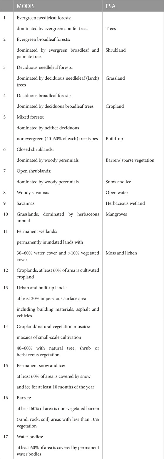
TABLE 1. Land cover type used by the MODIS and ESA WorldCover data sets.
The MODIS team quote an accuracy of 73.6% for their land cover type classification1, but this accuracy is likely to hide smaller regional accuracies depending on the individual land cover type. Zeng et al. (2015) e.g., compared the MODIS classification to the national land cover database of China (NLUD-C) and found an overall accuracy of 66.42%. For the Shrublands and the permanent wetlands land cover types, the obtained accuracies were however, well below 10%. This does not necessarily mean that the accuracy of the MODIS land cover type is below 10% for these land cover types, it could also be due to differences in the definition of these land cover type in the two databases.
The land cover types in the ESA WorldCover project are based on visual observations from the Sentinel-2 and Landsat satellites and on Synthetic Aperture Radar (SAR) observations from Sentinel-1 (Zanaga et al., 2021). These observations are combined to provide a global land cover product with a resolution of 10 m. Again, all 11 classifications (see Table 1) are fairly well represented with barren being the most abundant and mangroves being the least. The overall global accuracy is quoted to be 76.7%2.
For both land cover type data sets, the most likely land cover type was extracted for a 7 x 7 km foot print for each of the XCH4 measurement using the Google Earth Engine Python API (Google Earth Engine also provide interactive maps of the two land cover type data sets that allow for detailed inspection of the distributions of the different land cover types). Google Earth Engine stores data on multiple scales in image pyramids, where each pixel at a given level of the pyramid is computed from the aggregation of a 2x2 block of pixels at the next lower level. For a limit number (
2.4 XCH4 as a function of continent
The continent of the XCH4 measurements was obtained using a shapefile provided by Environmental Systems Research, Inc. and downscaled to 1% of the original resolution (∼100 km) in order to make the handling of 800 mio. data points feasible.
2.5 XCH4 as a function of season
Observations covering the period 20 December 2017 to 21 December 2020 were analysed. XCH4 levels were calculated as a function of season, where borders of the seasons were defined by summer and winter solar solstice as well as spring and fall equinox. The separation could have been based on the Gregorian calendar months instead, but astronomical calendar appears more universal.
Given that 3 years of observations were analysed means that each season contains observations from three different years.
3 Results and discussions
The global distributions of XCH4 as function of land cover type is shown in Figure 2. Figure 3 shows an example for the fall season, while Figure 4 & Figure 5 show how the fall season looks in Asia and Africa, respectively. All figures are based on the WFM-DOAS data retrieval algorithm and the MODIS land cover type. The rest of the figures, including all continents, for all seasons, both data retrieval algorithms and land cover type data sets can be found at [link to github] – including code for generating the figures.
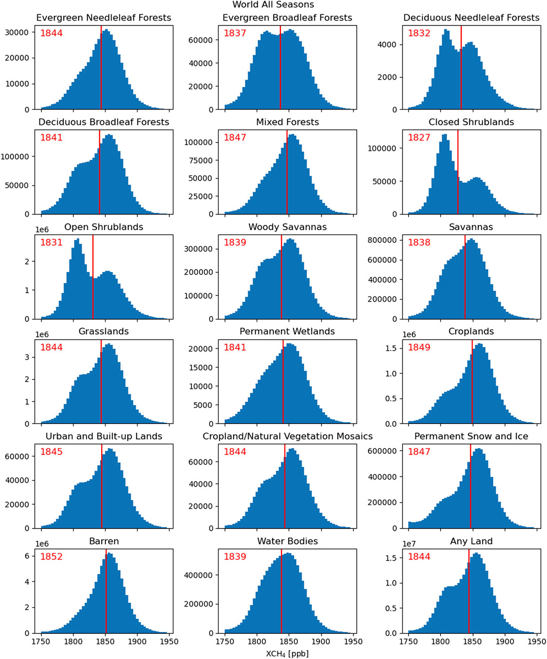
FIGURE 2. Global distribution of XCH4 retrieved with the WFM-DOAS algorithm as function of MODIS land cover type. The mean values of the distributions is indicated with the red lines and the red number in the upper left corner. The numbers on the y-axis (provided as multiple of 106 in some panels) represent the abselut numbers of cases in each bin. Cropland is the land cover type with the largest mean XCH4, while shrublands is the one with the smallest.
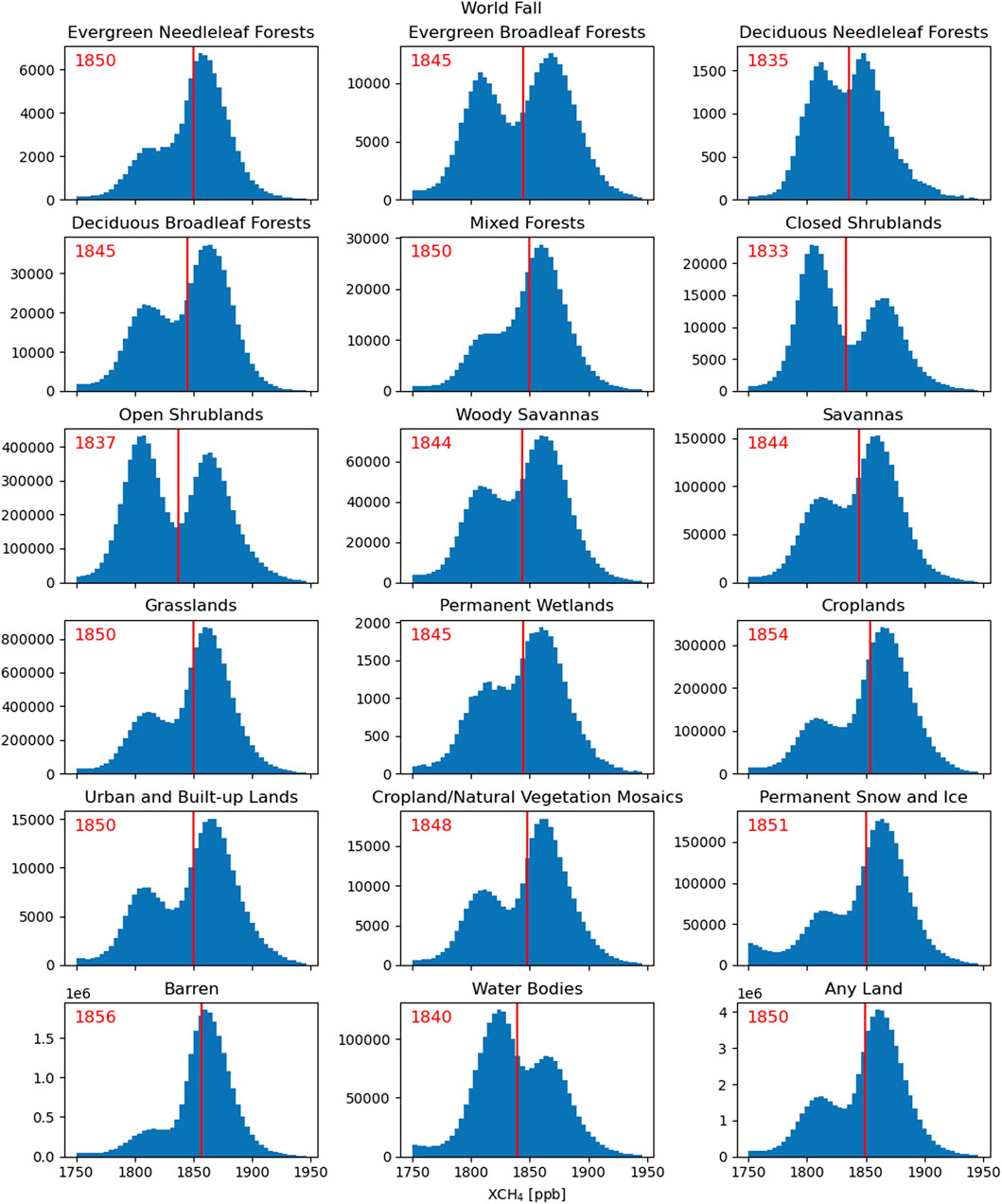
FIGURE 3. Similar to Figure 2, but here showing the global distribution of XCH4 retrieved with the WFM-DOAS algorithm as function of MODIS land cover type for the fall season. All of the land cover types show bimodal or asymmetric distributions. Most of these can be explained by significant lower methane emission during the fall and winter seasons in the southern hemisphere compared to the spring and summer season in the northern hemisphere. Similar bimodal or asymmetric distribution is seen for the global distribution obtained with the S5P-RemoTeC algorithm.
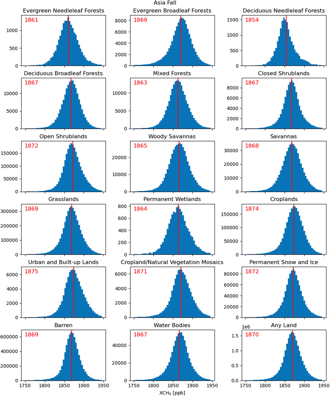
FIGURE 4. Similar to Figure 2, but here showing the distribution of XCH4 retrieved with the WFM-DOAS algorithm as function of MODIS land cover type for Asia for the fall season. Again, the largest mean XCH4 is seen from croplands.
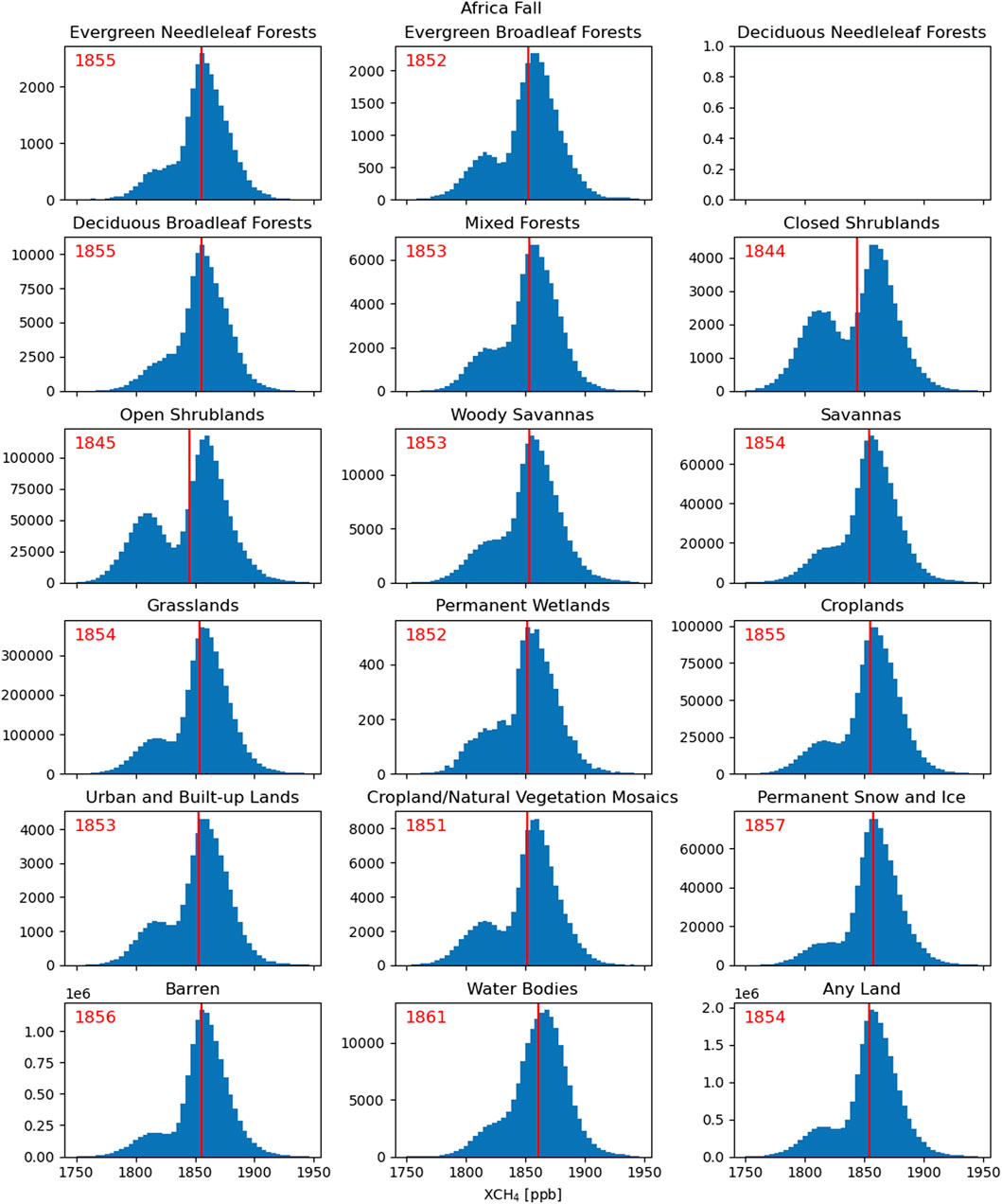
FIGURE 5. Similar to Figure 2, but here showing the distribution of XCH4 retrieved with the WFM-DOAS algorithm as function of MODIS land cover type for Africa for the fall season. Most of the land cover types show bimodal or asymmetric distributions.
Figure 2 reveals that none of the distributions of XCH4 retrieved with the WFM-DOAS algorithm as function of MODIS land cover type are normally distributed as could naively be expected given the large number of observations involved. All the distributions are clearly either bimodal or asymmetric. This is especially the case for deciduous needleleaf forest and open and closed shrublands. The effect is also seen using the ESA WorldCover land cover type, but it is less significant in the XCH4 measurements retrieved with the S5P-RemoTeC algorithm. For Africa the effect is however, present for both land cover data set and retrieval algorithms.
A bimodal or asymmetric distribution of XCH4 reflects that either the categorisation, with respect to land cover type, continent or season, has not been sufficiently detailed (mainly the case for the clearly bimodal distributions) or XCH4 do not follow a normal distribution (a log normal distribution would be a good candidate then).
The red lines in the distribution give that mean value of XCH4, which is also printed in the upper left corner. As can clearly be seen in the figures, the mean values should be handled with caution for these non-normal distributions. The mean values for all continents and all seasons are tabulated in Figure 6. The signatures in the XCH4 measurements retrieved with the S5P-RemoTeC algorithm and/or the MODIS land cover type data set in general looks very similar, with lower XCH4 levels observed over Australia and South America. For Australia and South America the highest XCH4 levels are observed in the summer seasons, while it is observed in the fall seasons for all other continents.
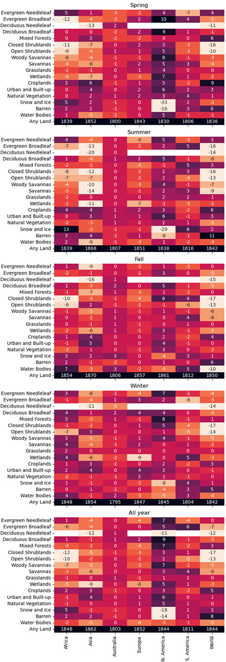
FIGURE 6. Colour coded matrices showing how the measured XCH4 values deviate of the mean as a function of land cover type, continent and season. The values for the ‘Any Land’ land cover types is given in ppb, while the other values are given as the deviation from this value in ppb. The complete names of the land cover types are given in Table 1. The XCH4 values were retrieved with the WFM-DOAS algorithm as function of MODIS land cover type.
One of the only significant differences between the results with the WFM-DOAS and the S5P-RemoTeC data retrieval algorithms is that while permanent snow and ice in general show lower than average XCH4 levels in the measurements retrieved with the S5P-RemoTeC algorithm, they show higher than average in the measurements retrieved with the WFM-DOAS algorithm. For the ESA WorldCover land cover type, the XCH4 levels are only lower than average for the measurements obtained with the S5P-RemoTeC algorithm. For the measurements obtained with the WFM-DOAS algorithm, the XCH4 levels over permanent snow and ice are very close to the average level. The reason for the difference in the XCH4 levels over permanent snow and ice obtained with the two different retrieval algorithms is likely do to differences in the handling of albedo effect in the two retrieval algorithms.
3.1 The interhemispheric gradient
The well know interhemispheric gradient in XCH4 with larger values in the northern hemisphere than in the southern (Hu et al., 2016; Schneising et al., 2019) is clearly visible in Figure 1. This gradient leads to the largest methane emission during the fall season as this broadly represents the shoulder season in the northern hemisphere.
The largest XCH4 levels are seen over Asia, followed by Europa, Africa and North America, while the XCH4 levels are clearly lower over South America and Australia (again reflecting the interhemispheric gradient). For the XCH4 levels retrieved with WFM-DOAS algorithm the highest levels are found over barren, which is likely linked to high XCH4 levels over barren in Africa and Asia (see Table 2). For the XCH4 levels retrieved with the RemoTeC algorithm the highest levels are found over build-up lands and croplands, this could be linked to high XCH4 levels over build-up lands in Europa and North America and over croplands in Africa and Asia. A relatively large number of observations from Africa are assigned as permanent snow and ice, but though Africa does indeed host three glaciers, this is likely do to misclassification between the permanent snow and ice and the barren land cover type. A similar, but opposite, effect is seen in Greenland and Arctic). In general, it was not possible to make solid conclusions about which land cover type that is responsible for the largest XCH4, but we see indication that barren, mangroves, croplands and build-up lands lead to higher XCH4 levels.
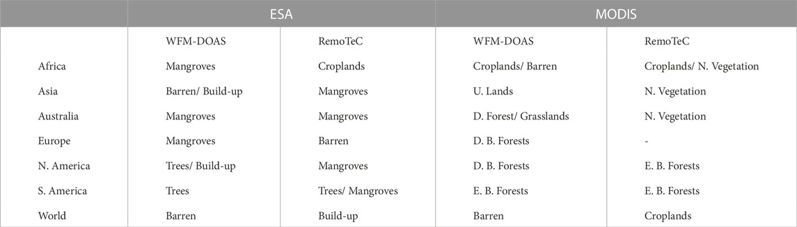
TABLE 2. Land cover types with the highest XCH4 levels as function of continent, land cover type data set and data retrieval algorithm. 5 land cover types: Evergreen Broadleaf Forests, Grasslands, Urban and Build-up Lands and Natural Vegetation Mosaics have similar XCH4 level for Europe using the RemoTeC algorithm and the MODIS data set.
3.2 Low XCH4 levels over wetlands
The results for the lowest XCH4 levels are less ambiguous. Here the lowest levels are seen over snow and ice, shrublands, moss and lichen and wetlands (see Table 3). For snow and ice, shrublands and moss and lichen this agrees with expatriation (Oertel et al., 2016), but wetlands are believed to be a major source of methane emission as they provide a habitat for methanogenic bacteria that produce methane during their decomposition of organic material. Wetlands are especially well suited as habitats for methanogenic bacteria as they provide an oxygen-free environment and abundant amounts of organic material (Zehnder, 1978). Methanotrophic bacteria are, on the other hand, capable of consuming methane, which, a long with dependencies on other factors such as temperature, pH and salinity, makes it hard to assess the net methane budget associated with wetlands (Segers, 1998).
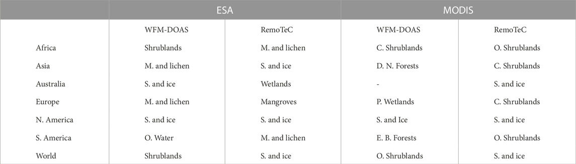
TABLE 3. Land cover types with the lowest XCH4 levels as function of continent, land cover type data set and data retrieval algorithm. 4 land cover types: Closed Shrublands, Croplands, Permanent Snow and Ice, Barren have similar XCH4 level for Australia using the WFM-DOAS algorithm and the MODIS data set.
The general lower than average XCH4 levels over wetlands are found with both land cover data sets and retrieval algorithms (see Table 4; Figure 7), except for North America, South America and Australia. In general, the methane emission from South America and Australia is very low and follow a different trend than the rest of the world (see Figure 8) – the reason being that these two continents are located on the southern hemisphere and that most methane sources, artificial and natural, lies in the northern hemisphere (Volodin, 2015), but for North America the difference contradicts the common model, where tropical wetlands are expected to emit more methane, than wetlands at higher latitudes as the higher temperatures will lead to more biological activity (Lunt et al., 2019). An explanation for this disagreement could be that the larger temperatures lead to not only more methanogenic bacteria, but also more methanotrophic bacteria (Wu et al., 2010) or alternatively that the lower temperatures in North America compared to the tropical regions lead to less methanotrophic bacteria activity.
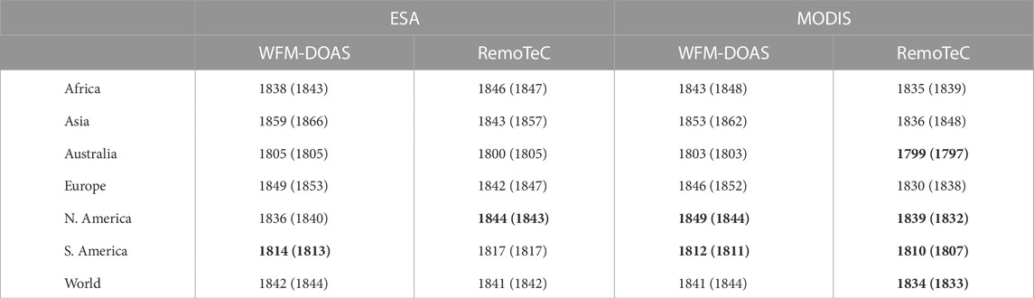
TABLE 4. XCH4 levels (in ppb) over wetlands as function of continent, land cover type data set and data retrieval algorithm. The numbers in brackets give the mean XCH4 levels for any land cover type. In general the XCH4 levels are found to be comparable to or lower than the mean level of any land cover type – except for 8 (out of 28) cases that are marked in boldface.
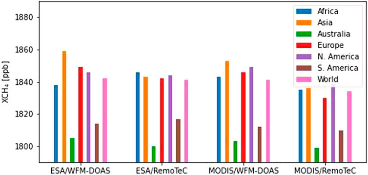
FIGURE 7. Bar plot of XCH4 levels over wetlands as function of continent, land cover type data set and data retrieval algorithm. The values used in the plot are given in Table 4.
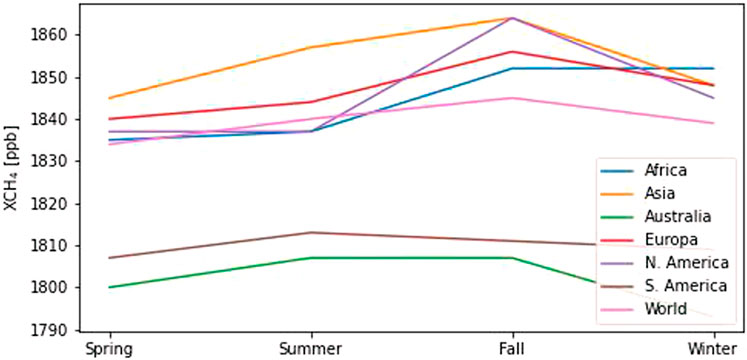
FIGURE 8. Annual variability of the absolute XCH4 levels over wetlands as function of continent. All continents, except for Australia and South America follows an annual cycle with high values in the fall and low levels in the spring. The levels over Australia and South America are seen to be lower and off phase with the rest of the world.
Though the general lower than average XCH4 levels over wetlands are found with both land cover data sets and retrieval algorithms, we cannot rule out that the discrepancy could be due to misclassification, problems with the low spatial resolution of the XCH4 measurements or biases in the data retrieval algorithms coursed by the low albedo of wetlands. However, redoing the analysis with observations from, e.g., the Thermal And Near-infrared Sensor for carbon Observation (TANSO) Fourier Transform Spectrometer (FTS) on the Greenhouse gases Observation Satellite (GOSAT) would be beyond the scope of this paper. Also, XCH4 levels from GOSAT have been compared to observations from Sentinel-5P by Lorente et al. (2021) and Yu et al. (2022), who both find a high degree of agreement.
Observations from both GOSAT and Sentinel-5P have been used to estimate methane emission from wetlands. In general, these studies find lower posterior emissions compared to prior emissions from, e.g., WetCHART (Bloom et al., 2017). This is in agreement with the lower than average XCH4 levels over wetlands that we find.
Maasakkers et al. (2019) used inversion of GOSAT observations to assess global methane emissions and found slightly lower posterior emission compared to prior emission based on WetCHAR for Southern US. This was explained by low soil organic carbon in these ecosystems. Yu et al. (2022) preformed a similar analysis, but this time using Sentinel-5P observations and found similar downward correction of the posterior emissions compared to the prior emissions in WetCHART for North America.
Methane emission for central Africa were estimated by both Lunt et al. (2019) using GOSAT observations and Pandey et al. (2021) using observations from Sentinel-5P. Lunt et al. (2019) found a methane emission that were 60% smaller than the WetCHART estimate for the Congo Basin, where 90% of the methane emission is expected to originate from wetlands (Bloom et al., 2017). The opposite scenario was however, observed for the South Sudan’s wetlands, where methane emissions levels four times higher than WetCHART were observed. The last result was confirmed by Pandey et al. (2021) using observations from Sentinel-5P and the data driven approach by Buchwitz et al. (2017).
Lunt et al. (2019) found the highest emission in the June-November months, while Pandey et al. (2021) found it in the December to February months, which is generally in agreement with the result presented here, where the highest concentrations are seen in the October-March months. As analysed by Pandey et al. (2021) there is a discrepancy in the seasonal change of the methane emission in the satellite observations and the WetCHART model that could be explained by a higher temperature dependence of the methane emission than suggested by the WetCHART models.
Ma et al. (2021) compared wetland models with emission fluxes from the GOSAT satellite and found that 72% of the global methane emission originates from tropical wetlands, but that the temperature sensitivity of the methane emission from wetlands was in general lower than expected. Together with our result, this indicates that the methane emission from wetlands is also controlled by other factors that just latitude and temperature.
Saunois et al. (2020) estimated the methane emission from wetlands to be between 100 and 217 Tg CH4 per year. Making it account for between 11 and 38% of the global methane emission. In the land cover classifications used here, permanent wetlands makes up less than 2% of the samples (excluding the oceans). Therefore, in order for the permanent wetlands to account for even 10% of the global methane emission, the relative emission from permanent wetlands would have to be significant larger than most other land cover types. However, the smaller than average XCH4 levels observed over wetlands in this study suggest the opposite. This is an example of a peculiarity, as described in the introduction, where the XCH4 measurements points in a different direction than the methane emission estimates obtained with inversion. The peculiarity could be due to some not well understood mechanism in the inversion that would transport methane away from the permanent wetlands or it could be due to an overestimation of the prior methane emission from permanent wetlands used in the inversion. Our study thus reveals a need to investigate if wetlands are modelled correctly in the different inversion models used to estimate methane emissions.
Another factor that influences the global XCH4 distribution is the interhemispheric transport of air masses. In a combined analysis using XCH4 observations from GOSAT with atmospheric simulations at global scale, Belikov et al. (2022) identified the location of longitudinal zones of active interhemispheric transport over tropical South America, tropical Africa and Southeast Asia, where the methane mass fluxes are transported toward the south all year long.
Is it somewhat puzzling that while the XCH4 levels over wetlands general seems to be lower than average, the levels of mangroves seem to be higher and the two land cover types appears very similar. The mangrove land cover category is only found in the ESA WorldCover land cover type and in general with low abundances, so the mangrove measurements a less reliable than the observations of wetlands.
The fact that only permanent wetlands were included in the analysis could have an effect on the results, but the effect would be in the wrong direction as permanent wetlands have lower concentrations of oxygen compared to other wetland types and therefore would favour methanogenic over methanotrophic bacteria.
It is possible that the low spatial resolution of the XCH4 observations means that many small permanent wetlands are not included in the analysed wetlands (Hondula et al., 2021). It is however, not clear how that should change the general picture observed here that wetlands in general show smaller than average XCH4 levels.
North America shows larger variability in the relative XCH4 levels over wetlands than other land cover types compared to other continents (see Figure 6). but the absolute variability is smaller (see Figure 8). In other words, XCH4 varies out of phase with other land cover types in North America. These are mainly barren and permanent snow and ice, which shows clear bimodal distributions with high values in fall and winter and low values in spring and summer. As barren and permanent snow and ice are more common land cover types than wetlands, the variability of these land cover types dominated the integrated variability over North America thereby off phasing the variability over wetlands.
3.3 The annual methane cycle
Africa constitute a special case in the analysis as it is located on both the northern and southern hemisphere and as many of the distributions seems to be clearly bimodal. The main contribution to the observed XCH4 over Africa is however, attributed to the land north of equator (see Figure 1). Bimodal distributions are especially pronounce for evergreen broadleaf forests, shrublands, savannas and barrens. The bimodal distributions can all be explained by significantly higher XCH4 levels during the fall and winter seasons compared to the spring and summer seasons (See an example of the fall season in Figure 5). The low XCH4 peak of the bimodal distributions is strongest in the spring season and then broadens out during the summer season. In the fall season a high XCH4 peak appears together with the low XCH4 peak and during the winter season only the high XCH4 peak is left.
Generally, wetlands emit methane when they are wet and take up methane when they are dry. It is therefore interesting to look at the annual variability that is shown in Figure 8. The figure shows that all continents, except for Australia and South America, follows a trend with high XCH4 levels over wetlands during the fall season and low during the spring season. This trend is strongest for Asia, which also have the strongest rain season. This trend can also be explained by the fact that the methanogenic bacteria have more organic material available for decomposition in the fall season and this effect might be more important for continent with no strong rain season.
The observed annual cycle in XCH4 levels over wetlands is in agreement with other studies covering North America (Javadinejad et al., 2019) that also see higher emission during fall and winter and India (Chandra et al., 2017; Ganesan et al., 2017) that see peak concentrations in July and August. A global study (Tian et al., 2015) shows results in agreement with the results presented here.
The far largest XCH4 levels are seen in Asia. This can be explained by the fact that XCH4 levels are larger for croplands in Asia than in any other continent. This could be due to atmospheric transport mechanisms, but it could also be due to rise production taking up a large fraction of croplands in Asia (Zhang G. et al., 2020) and that croplands is an abundant land cover type in Asia. In fact, methane emission from rice cultivation in top methane-emitting countries such as China and India, with roughly 20 and 10% of global share, accounting for over 4 and 1% of total methane emission, respectively (Crippa et al., 2020). This would also explained why Asia experience peak XCH4 levels during the summer and fall season, while Africa, Europe and North America experience peak XCH4 levels during fall and winter. The reason being the multiple annual rice seasons are common and therefore the methane emission would tend to follow the mean temperature more closely in Asia. In Africa, Europe and North America, where multiple harvest seasons are not that common, the methane emission would follow the grow seasons more closely, with low emission during spring and summer were the crops grow and large emission during fall and winter due to the increase biological activity in the remaining roots and little oxidation of methane. Another reason for the earlier peak in XCH4 levels in Asia could be increased precipitation with the monsoon, which reduces the methane uptake of the croplands (Oertel et al., 2016).
4 Conclusion
We have used 3 years of XCH4 measurements (over 800 mio. measurements) from the TROPOMI instrument on Sentinel-5P to evaluate the XCH4 level as function of geographic, land cover type and season. The XCH4 values were obtained using the WFM-DOAS Schneising et al. (2019) and the S5P-RemoTeC Lorente et al. (2021) retrieval algorithms and the land cover types were obtained from MODIS (Friedl et al., 2010) and from the ESA WorldCover project.
The main finding of the study is that the average XCH4 levels over wetlands are generally lower than the average level for all land cover types – except for North America, South America and Australia. The reason for this could be that the methane emission from wetlands is compensated by a methane sink and that wetlands thus contribute less to the global methane budget than previously thought. We can however, not rule out that the discrepancy could be due to misclassification, problems with the low spatial resolution of the XCH4 measurements or biases in the data retrieval algorithms coursed by the low albedo of wetlands. Though the general lower than average XCH4 levels over wetlands are found with both land cover data sets and retrieval algorithms, we only analyse observations from one instrument. Before the result is verified with observations from other instruments, e.g., the TANSO-FTS instrument on GOSAT and in situ observations, we those recommend that the TROPOMI XCH4 measurements over wetlands are handled with caution.
Especially for Africa, a strong annual methane cycle is observed with significant higher XCH4 levels during the fall and winter seasons compared to the spring and summer seasons. This suggests that the XCH4 levels follow the annual growing seasons, with low emission during spring and summer were the crops grow and high emission during fall and winter due to the increased biological activity in the remaining roots and little oxidation of methane. Similar but smaller methane cycles are seen in North America and Europe.
In Asia the methane cycles is shifted a few months forward. This can be explained by the multiple annual rice seasons in Asia, which would make the XCH4 levels in Asia follow the temperatures more closely than the annual growing seasons.
Data availability statement
Publicly available datasets were analyzed in this study. This data can be found here: https://www.iup.uni-bremen.de/carbon_ghg/products/tropomi_wfmd/ and here https://www.sron.nl/earth-data-access. Python codes for analysing the XCH4 measurements and for generating the plots in this paper are available on https://github.com/karoff/methanedistributions along with pregenerated histograms for all seasons and all continents.
Author contributions
CK designed the study, made the analysis and wrote the paper. AV-V contributed to the analysis of the results and writing of the paper.
Funding
This work was supported by a research grant (40709) from Villum Fonden.
Acknowledgments
We thank the reviewers for comments and suggestions that helped improve the paper.
Conflict of interest
The authors declare that the research was conducted in the absence of any commercial or financial relationships that could be construed as a potential conflict of interest.
Publisher’s note
All claims expressed in this article are solely those of the authors and do not necessarily represent those of their affiliated organizations, or those of the publisher, the editors and the reviewers. Any product that may be evaluated in this article, or claim that may be made by its manufacturer, is not guaranteed or endorsed by the publisher.
Footnotes
1https://modis-land.gsfc.nasa.gov/ValStatus.php?ProductID=MCD12.
2https://esa-worldcover.org/en/about/about.
References
Belikov, D. A., Saitoh, N., and Patra, P. K. (2022). An analysis of interhemispheric transport pathways based on three-dimensional methane data by gosat observations and model simulations. J. Geophys. Res. Atmos. 127, e2021JD035688. doi:10.1029/2021jd035688
Bloom, A. A., Bowman, K. W., Lee, M., Turner, A. J., Schroeder, R., Worden, J. R., et al. (2017). A global wetland methane emissions and uncertainty dataset for atmospheric chemical transport models (wetcharts version 1.0). Geosci. Model Dev. 10, 2141–2156. doi:10.5194/gmd-10-2141-2017
Buchwitz, M., Schneising, O., Reuter, M., Heymann, J., Krautwurst, S., Bovensmann, H., et al. (2017). Satellite-derived methane hotspot emission estimates using a fast data-driven method. Atmos. Chem. Phys. 17, 5751–5774. doi:10.5194/acp-17-5751-2017
Chandra, N., Hayashida, S., Saeki, T., and Patra, P. K. (2017). What controls the seasonal cycle of columnar methane observed by gosat over different regions in India? Atmos. Chem. Phys. 17, 12633–12643. doi:10.5194/acp-17-12633-2017
Crippa, M., Solazzo, E., Huang, G., Guizzardi, D., Koffi, E., Muntean, M., et al. (2020). High resolution temporal profiles in the emissions database for global atmospheric research. Sci. Data 7, 121. doi:10.1038/s41597-020-0462-2
de Gouw, J. A., Veefkind, J. P., Roosenbrand, E., Dix, B., Lin, J. C., Landgraf, J., et al. (2020). Daily satellite observations of methane from oil and gas production regions in the United States. Sci. Rep. 10, 1379. doi:10.1038/s41598-020-57678-4
Friedl, M. A., Sulla-Menashe, D., Tan, B., Schneider, A., Ramankutty, N., Sibley, A., et al. (2010). Modis collection 5 global land cover: Algorithm refinements and characterization of new datasets. Remote Sens. Environ. 114, 168–182. doi:10.1016/j.rse.2009.08.016
Friedlingstein, P., O’Sullivan, M., Jones, M. W., Andrew, R. M., Hauck, J., Olsen, A., et al. (2020). Global carbon budget 2020. Earth Syst. Sci. Data 12, 3269–3340. doi:10.5194/essd-12-3269-2020
Ganesan, A. L., Rigby, M., Lunt, M. F., Parker, R. J., Boesch, H., Goulding, N., et al. (2017). Atmospheric observations show accurate reporting and little growth in India’s methane emissions. Nat. Commun. 8, 836. doi:10.1038/s41467-017-00994-7
Hondula, K. L., DeVries, B., Jones, C. N., and Palmer, M. A. (2021). Effects of using high resolution satellite-based inundation time series to estimate methane fluxes from forested wetlands. Geophys. Res. Lett. 48, e2021GL092556. doi:10.1029/2021gl092556
Hu, H., Hasekamp, O., Butz, A., Galli, A., Landgraf, J., Aan de Brugh, J., et al. (2016). The operational methane retrieval algorithm for tropomi. Atmos. Meas. Tech. 9, 5423–5440. doi:10.5194/amt-9-5423-2016
Ialongo, I., Stepanova, N., Hakkarainen, J., Virta, H., and Gritsenko, D. (2021). Satellite-based estimates of nitrogen oxide and methane emissions from gas flaring and oil production activities in sakha republic, Russia. Atmos. Environ. X 11, 100114. doi:10.1016/j.aeaoa.2021.100114
Javadinejad, S., Eslamian, S., and Ostad-Ali-Askari, K. (2019). Investigation of monthly and seasonal changes of methane gas with respect to climate change using satellite data. Appl. Water Sci. 9, 180. doi:10.1007/s13201-019-1067-9
Lorente, A., Borsdorff, T., Butz, A., Hasekamp, O., aan de Brugh, J., Schneider, A., et al. (2021). Methane retrieved from tropomi: Improvement of the data product and validation of the first 2 years of measurements. Atmos. Meas. Tech. 14, 665–684. doi:10.5194/amt-14-665-2021
Loveland, T. R., and Belward, A. S. (1997). The igbp-dis global 1km land cover data set, discover: First results. Int. J. Remote Sens. 18, 3289–3295. doi:10.1080/014311697217099
Lunt, M. F., Palmer, P. I., Feng, L., Taylor, C. M., Boesch, H., and Parker, R. J. (2019). An increase in methane emissions from tropical Africa between 2010 and 2016 inferred from satellite data. Atmos. Chem. Phys. 19, 14721–14740. doi:10.5194/acp-19-14721-2019
Lunt, M. F., Palmer, P. I., Lorente, A., Borsdorff, T., Landgraf, J., Parker, R. J., et al. (2021). Rain-fed pulses of methane from east Africa during 2018–2019 contributed to atmospheric growth rate. Environ. Res. Lett. 16, 024021. doi:10.1088/1748-9326/abd8fa
Ma, S., Worden, J. R., Bloom, A. A., Zhang, Y., Poulter, B., Cusworth, D. H., et al. (2021). Satellite constraints on the latitudinal distribution and temperature sensitivity of wetland methane emissions. AGU Adv. 2, e2021AV000408. doi:10.1029/2021av000408
Maasakkers, J. D., Jacob, D. J., Sulprizio, M. P., Scarpelli, T. R., Nesser, H., Sheng, J.-X., et al. (2019). Global distribution of methane emissions, emission trends, and oh concentrations and trends inferred from an inversion of gosat satellite data for 2010–2015. Atmos. Chem. Phys. 19, 7859–7881. doi:10.5194/acp-19-7859-2019
Nisbet, E. G., Dlugokencky, E. J., Manning, M. R., Lowry, D., Fisher, R. E., France, J. L., et al. (2016). Rising atmospheric methane: 2007-2014 growth and isotopic shift. Glob. Biogeochem. Cycles 30, 1356–1370. doi:10.1002/2016GB005406
Oertel, C., Matschullat, J., Zurba, K., Zimmermann, F., and Erasmi, S. (2016). Greenhouse gas emissions from soils—A review. Geochemistry 76, 327–352. doi:10.1016/j.chemer.2016.04.002
Pandey, S., Houweling, S., Lorente, A., Borsdorff, T., Tsivlidou, M., Bloom, A. A., et al. (2021). Using satellite data to identify the methane emission controls of south Sudan’s wetlands. Biogeosciences 18, 557–572. doi:10.5194/bg-18-557-2021
Parker, R. J., Boesch, H., McNorton, J., Comyn-Platt, E., Gloor, M., Wilson, C., et al. (2018). Evaluating year-to-year anomalies in tropical wetland methane emissions using satellite ch4 observations. Remote Sens. Environ. 211, 261–275. doi:10.1016/j.rse.2018.02.011
Reuter, M., Buchwitz, M., Schneising, O., Noël, S., Bovensmann, H., Burrows, J. P., et al. (2020). Ensemble-based satellite-derived carbon dioxide and methane column-averaged dry-air mole fraction data sets (2003–2018) for carbon and climate applications. Atmos. Meas. Tech. 13, 789–819. doi:10.5194/amt-13-789-2020
Saunois, M., Jackson, R. B., Bousquet, P., Poulter, B., and Canadell, J. G. (2016). The growing role of methane in anthropogenic climate change. Environ. Res. Lett. 11, 120207. doi:10.1088/1748-9326/11/12/120207
Saunois, M., Stavert, A. R., Poulter, B., Bousquet, P., Canadell, J. G., Jackson, R. B., et al. (2020). The global methane budget 2000–2017. Earth Syst. Sci. Data 12, 1561–1623. doi:10.5194/essd-12-1561-2020
Schneising, O., Buchwitz, M., Reuter, M., Bovensmann, H., Burrows, J. P., Borsdorff, T., et al. (2019). A scientific algorithm to simultaneously retrieve carbon monoxide and methane from tropomi onboard sentinel-5 precursor. Atmos. Meas. Tech. 12, 6771–6802. doi:10.5194/amt-12-6771-2019
Segers, R. (1998). Methane production and methane consumption: A review of processes underlying wetland methane fluxes. Biogeochemistry 41, 23–51. doi:10.1023/a:1005929032764
Tian, H., Chen, G., Lu, C., Xu, X., Ren, W., Zhang, B., et al. (2015). Global methane and nitrous oxide emissions from terrestrial ecosystems due to multiple environmental changes. Ecosyst. Health Sustain. 1, 1–20. doi:10.1890/EHS14-0015.1
Varon, D. J., Jacob, D. J., Sulprizio, M., Estrada, L. A., Downs, W. B., Shen, L., et al. (2022). Integrated methane inversion (imi 1.0): A user-friendly, cloud-based facility for inferring high-resolution methane emissions from tropomi satellite observations. Geosci. Model Dev. 15, 5787–5805. doi:10.5194/gmd-15-5787-2022
Volodin, E. M. (2015). Influence of methane sources in northern hemisphere high latitudes on the interhemispheric asymmetry of its atmospheric concentration and climate. Izvestiya, Atmos. Ocean. Phys. 51, 251–258. doi:10.1134/S0001433815030123
Wu, X., Yao, Z., Brüggemann, N., Shen, Z., Wolf, B., Dannenmann, M., et al. (2010). Effects of soil moisture and temperature on co2 and ch4 soil–atmosphere exchange of various land use/cover types in a semi-arid grassland in inner Mongolia, China. Soil Biol. Biochem. 42, 773–787. doi:10.1016/j.soilbio.2010.01.013
Yu, X., Millet, D. B., Henze, D. K., Turner, A. J., Delgado, A. L., Bloom, A. A., et al. (2022). A high-resolution satellite-based map of global methane emissions reveals missing wetland, fossil fuel and monsoon sources. EGUsphere 2022, 1–37. doi:10.5194/egusphere-2022-948
Zanaga, D., Van De Kerchove, R., Daems, D., De Keersmaecker, W., Brockmann, C., Kirches, G., et al. (2021). Esa worldcover 10 m 2021 v200. Zenodo. doi:10.5281/zenodo.7254221
Zehnder, A. (1978). “Ecology of methane formation,” in Water pollution microbiology. Editor R. Mitchell (New York: J. Wiley and Sons), Vol. 2, 249–376.
Zeng, T., Zhang, Z., Zhao, X., Wang, X., and Zuo, L. (2015). Evaluation of the 2010 modis collection 5.1 land cover type product over China. Remote Sens. 7, 1981–2006. doi:10.3390/rs70201981
Zhang, G., Xiao, X., Dong, J., Xin, F., Zhang, Y., Qin, Y., et al. (2020). Fingerprint of rice paddies in spatial–temporal dynamics of atmospheric methane concentration in monsoon Asia. Nat. Commun. 11, 554. doi:10.1038/s41467-019-14155-5
Keywords: remote sensing, atmospheric methane, sentinel 5p, greenhous gases, wetlands, TROPOMI
Citation: Karoff C and Vara-Vela AL (2023) Data driven analysis of atmospheric methane concentrations as function of geographic, land cover type and season. Front. Earth Sci. 11:1119977. doi: 10.3389/feart.2023.1119977
Received: 09 December 2022; Accepted: 13 March 2023;
Published: 27 March 2023.
Edited by:
Can Li, University of Maryland, United StatesReviewed by:
Qiansi Tu, Karlsruhe Institute of Technology (KIT), GermanyBingkun Luo, Harvard University, United States
Copyright © 2023 Karoff and Vara-Vela. This is an open-access article distributed under the terms of the Creative Commons Attribution License (CC BY). The use, distribution or reproduction in other forums is permitted, provided the original author(s) and the copyright owner(s) are credited and that the original publication in this journal is cited, in accordance with accepted academic practice. No use, distribution or reproduction is permitted which does not comply with these terms.
*Correspondence: Christoffer Karoff, a2Fyb2ZmQGdlby5hdS5kaw==