Gas-bearing prediction of deep reservoir based on DNN embeddings

The extraction of gas-bearing information from the deeply underground reservoir is extremely difficult due to the weak seismic response and complicated gas distribution characteristics. To predict gas-bearing reservoirs efficiently, we developed a deep neural network (DNN) embedding-based gas-bearing prediction scheme. First, the cepstrum coefficient that is sensitive to hydrocarbons is computed using the raw seismic data. A DNN model inspired by the x-vector in speech recognition is designed, comprising the long short-term memory (LSTM) networks and two fully connected (FC) networks, stacked from the bottom to the top layer. Then, the cepstrum features are fed into the DNN for training and testing, and DNN embedding is extracted from the top layers after optimized network parameters are determined. Finally, the gas-bearing probability of the reservoir is predicted by calculating the cosine distance between pairs of DNN embeddings. When applied to synthetic seismic data, the proposed method offers greater than 90% accuracy at SNR > 3 dB. Besides, the predicted result applied in deep carbonate reservoirs in China’s Sichuan Basin is in basic agreement with the actual situation, demonstrating the certain feasibility of the proposed scheme.

1 Introduction

The targets for oil and gas exploration continue to develop to greater depths as the conventional technology for exploration in the petroleum industry advances. Deeply underground reservoirs are covered by massive thick sediments that have minimal physical differences from surrounding rocks, low porosity, strong non-homogeneity, and poor seismic response, making the distribution of oil and gas complicated. Traditional methods used to detect gas-bearing properties in reserves include the “bright spot” method (Hammond, 1974), AVO analysis (Hampson, 1991), and low-frequency shadowing (Taner et al., 1979). These methods are effective in specific scenarios (Cao et al., 2022), for example, bright spot technology is mainly useful in shallow unconsolidated clastic reservoirs, while AVO analysis technology is suitable for formations with a relatively simple and gentle structure. Low-frequency shadowing is mainly applied to lithologies that are already known. However, these traditional techniques are difficult to effectively quantify the complex and non-linear connection between seismic response and gas-bearing properties in deeply buried reservoirs.

Recently data-driven deep learning methods are widely used in geophysics for first-to-wave pickup (Liao et al., 2020; Qu et al., 2021), seismic data denoising (Wang and Chen, 2019; Liu et al., 2020; Liu et al., 2022), and seismic facies recognition (Tschannen et al., 2020; Liu et al., 2021). Due to the advantage of automatically characterizing complex multivariate non-linear relationships, DNN is also used for acquiring reservoir gas-bearing properties. For example, a deep neural network (DNN) model with several hidden layers (Yang et al., 2021; Zhang et al., 2022) is built for gas-bearing prediction by leveraging the capability of DNN to handle an end-to-end task. The convolution neural network (CNN), one of the most promising DNN approaches for geophysics issues, has been trained for extracting oil and gas properties (Song et al., 2022). The characteristics of the reservoir are reflected in the comparison with the surrounding rock layers above and below it. However, these methods primarily concentrate on learning the gas-bearing information of the target layer, and the contextual relationship between the seismic waveforms is not given the same level of attention.

Although there have been many deep learning methods applied to the processing and interpretation of seismic data, few studies have focused on hydrocarbon detection. This article presents an innovative experiment that uses neural networks to quantitatively identify the gas-bearing information in seismic records based on the similarities between seismic and acoustic data. The similarities are manifested in two aspects (Xie et al., 2017). First, seismic primary waves and acoustic waves can be considered as the same kind of wave since their propagation in the elastic medium follows the same physical laws. In addition, both can be characterized by convolutional models. The seismic record can be seen as a convolution of stratigraphic reflection coefficients and waves, and the acoustic record can be regarded as the convolution of the vocal cord excitation and the vocal tract. Therefore, speech feature parameters can be integrated into seismic data processing. For example, cepstrum is applied to the computation for thin beds thickness (Hall, 2006) and gas-bearing detection (Tian and Cao, 2011; Xue et al., 2016), and the Linear Prediction cepstral Coefficient (LPCC) is utilized for seismic facies analysis (Xie et al., 2016). With the demand for improving speaker recognition technology, the novel speech characteristics generated by DNN have grown increasingly prominent. Especially, the x-vector, namely, DNN embedding, captures accurately the vocal information of speakers by translating arbitrary-length inputs into fixed-length embeddings, making it effective for short-time records (Snyder et al., 2017; Snyder et al., 2018). Therefore, this article utilizes DNN embedding to predict gas-bearing reservoirs due to its outstanding feature extraction ability for short seismic responses.

Facing the problems of weak seismic response and thin thickness of deep buried reservoirs, we have improved and modified the DNN model prediction method. First of all, for data preparation, we obtained datasets tailored to seismic data characteristics. And the cepstrum is employed as the DNN input since it has been shown sensitive to the response of the gas-bearing layer (Cao et al., 2011; Cao et al., 2019). Secondly, in terms of the DNN model, it employed long short-term memory (LSTM) networks as the bottom layer to contextualize feature learning and the two FC layer as the primary top layer for embedding extraction. Thirdly, to visualize the gas-bearing distribution, the backend of the model outputs DNN embedding pairs’ similarity using cosine distance. Evaluations based on both synthetic and actual seismic records from China’s Sichuan Basin demonstrate that our method has significant advantages over traditional SVM-based approach (Tian and Cao, 2011).

2 Materials and methods

Since acoustic waves and seismic waves share certain similarities described above, it is theoretically possible to apply speaker recognition technology to identify certain geological bodies, such as gas-bearing reservoirs. Speaker recognition identifies the speaker by acquiring common features in numerous utterances. Similarly, when common characteristics in seismic records are extracted for gas-bearing prediction, the gas-bearing reservoir corresponds to the speaker, and the seismic records correspond to the acoustic records. Nonetheless, these two records differ, and the technique cannot be transferred directly. Based on the characteristics of the seismic data, the proposed scheme displayed in Figure 1 is designed for seismic records.

FIGURE 1

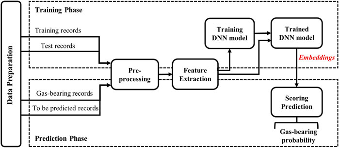
FIGURE 1. Workflow of gas-bearing prediction for the deep reservoir based on DNN Embeddings.

2.1 Data preparation

When preparing the dataset, the difference in attenuation, repeatability, and frequency of seismic data must be taken into consideration (Cao et al., 2011; Cao et al., 2019).

2.1.1 Attenuation

The speaker is the source of speech records, and there is no attenuation as time passes. While the source of seismic records is the reflection or dispersion of the seismic source signal, which is a secondary source and decays with increasing recording time. Therefore, amplitude-preserving processing is necessary (Gao et al., 2022) to remove the effects of spherical diffusion and inelastic attenuation.

2.1.2 Repeatability

The “voiceprint” characteristic is repeated in a single utterance for acoustic records, and a single speaker can give numerous bits of utterances. Seismic records are continuous and redundant (Coléou et al., 2003). The continuity means that the geological condition over a certain spatial range is similar, which is the foundation of tectonic and stratigraphic interpretation. The redundancy exists in some spreading information of wavefront propagation that occurs in both longitudinal and lateral directions. To sum up, seismic records within a certain lateral and longitudinal range can be approximately regarded as the response of a similar reservoir.

2.1.3 Short-time smoothness

Speech recognition decomposes acoustic records into frames, and each frame can be regarded as a smooth signal. The frequency of seismic records is much lower than the frequency of acoustic records, so the seismic response can only be considered smooth when the time window is narrow. Since the characteristics of the reservoir are reflected in the comparison with the surrounding rock above and below it, the window can be expanded within a reasonable range.

2.2 Pre-processing

Before extracting the features from the raw seismic records, pre-processing needs to be implemented. Pre-processing consists of pre-emphasis, framing, and windowing operations. Except for important parameter values which are specially set according to our practical experience, the process is consistent with speech signal processing (Muda et al., 2010).

2.3 Feature extraction

The cepstrum feature is selected as the input feature for DNN to extract stratigraphic response features by taking into account the following factors. Firstly, the cepstrum feature is sensitive to gas-bearing characteristics in hydrocarbon prediction (Cao et al., 2011; Cao et al., 2019). Then, the cepstrum has a simple derivation process compared with the widely used Mel Frequency Cepstral Coefficient (MFCC) and the FilterBank (FBank) (Zheng et al., 2001; Wang et al., 2014) in speech recognition, which is represented in Figure 2. Moreover, the cepstrum also can simplify the relation between seismic wavelet and stratigraphic reflection coefficients which will be demonstrated below.

FIGURE 2

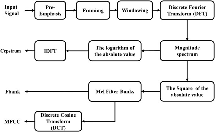
FIGURE 2. The extraction process of MFCC, FBank, and Cepstrum features.

The cepstrum is the real component of the Inverse Discrete Fourier transform (IDFT) for a time domain sequence’s logarithmic amplitude spectrum, which is a homomorphic transform. Assume that $\left[x\left(n\right),n=\mathrm{0,1,2},\dots ,N-1\right]$ is a time domain discrete signal with N sampling points, in which $n$ is the discrete sampling of time. The cepstrum of $x\left(n\right)$ is described by the equation below.

$\overline{x\left(n\right)}=Re\left[F^{-1}\left(\mathit{log}\left|F\left(x\left(n\right)\right)\right|\right)\right](1)$

In the Formula 1, $F$ denotes Discrete Fourier transform (DFT), $F^{-1}$ denotes IDFT, and $\left|\bullet \right|$ denotes the mode-taking operation. Besides, $F\left(x\left(n\right)\right)$ can be written as $X\left(k\right)$, in which $X\left(\bullet \right)$ represents the frequency domain signal of $x\left(n\right)$ and $\left[k=\mathrm{0,1,2},\dots ,N-1\right]$ is the discrete sampling of the analog frequency.

The discrete seismic signal is expressed as the following equation based on the seismic record convolutional model.

$s\left(n\right)=w\left(n\right)\ast r\left(n\right)(2)$

In Formula 2, $r\left(n\right)$ is the stratigraphic reflection coefficient, $w\left(n\right)$ is the seismic wavelet, which is typically the Ricker wavelet, and $*$ is the convolution operation. According to Formula 1, the cepstrum domain parameters of the seismic record can be computed as follows.

$Re\left[F^{-1}\left(\mathit{log}\left|S\left(k\right)\right|\right)\right]=Re\left[F^{-1}\left(\mathit{log}\left|W\left(k\right)\right|\right)\right]+Re\left[F^{-1}\left(\mathit{log}\left|R\left(k\right)\right|\right)\right](3)$

In Formula 3, $S\left(k\right),W\left(k\right)$ and $R\left(k\right)$ are the spectrum of seismic record, seismic wavelet, and reflection coefficients, respectively. In the cepstrum domain, the correlation between seismic wavelet and reflection coefficient becomes simple, i.e., the convolutional relationship in the time domain becomes a sum of two in the cepstrum. Before input to DNN, the energy, mean, and variance of the cepstrum are added to the first three dimensions of each frame feature to enhance the dimensionality of the feature parameters.

2.4 Training DNN model

The DNN architecture is comparable to the network architecture in the Kaldi Voxceleb recipe (Kumar et al., 2020), which consists of the frame-level layer, segment-level layer, and softmax layer as shown in Figure 3. The first frame-level layers in Kaldi consist of time-delay neural networks (TDNN) with a context and are utilized for learning repetitive features in multiple frames. In this paper, we suggest switching from TDNN to LSTM networks, because that LSTM can automatically learn long-term relationships between sequences and have a similar time-delay function. And then, the segment-level layer gathers information from the context to recognize the segment characteristics of seismic records, among which, a statistical pooling layer combines the mean and standard deviation from the output of frame 5, and two fully connected (FC) layers can be utilized to extract embedding after the training is completed. The number of hidden layer nodes is reduced according to the length of the frame there because of the smaller size of seismic data. The top softmax layer outputs the maximum posterior probability for each reservoir type and it is no longer required once the DNN training is complete. In addition, each layer has a batch normalization (BN) layer and a rectified linear units (ReLUs) activation function to enhance DNN performance.

FIGURE 3

FIGURE 3. The DNN architecture of the proposed scheme.

2.5 Scoring prediction

The front of our proposed method is used for extracting seismic embeddings. Once the DNN model has been trained, two FC layers produce the embeddings, which are the representations of the seismic records. The output of segment 1 is Embedding a (EMa), which is immediately output on the statistics layer, while the output of segment 2 is Embedding b (EMb), which is extracted from the FC layer after the ReLUs layer.

The back-end in our scheme is scoring prediction based on the embedding similarity. The embedding of the gas reserve is derived from the seismic record adjacent to the gas-bearing well, which is indicated as $E{M}_g$. Similarly, the embedding for a seismic record to be predicted is labeled as $E{M}_p$. The embedding similarity between $E{M}_g$ and $E{M}_p$ represents the gas-bearing probability of the corresponding layer where the seismic records are located. The normalized cosine distance is employed in this research to represent the similarity, which is described by the equation below.

$\mathit{Cos}\left(E{M}_g,E{M}_p\right)=0.5\times \frac{E{M}_g\bullet E{M}_p}{‖E{M}_g‖\bullet ‖E{M}_p‖}+0.5(4)$

3 The experiment of the geological model

A geological attenuation model was developed to test the effectiveness of gas-bearing prediction with the dispersive viscosity equation (He et al., 2009). By referring to reservoir logging parameters and geological data in the Sichuan Basin, China, the geological model was designed and its parameters were configured in Table 1. In Figure 4A, Layer ③, ④, and ⑤ are the water-bearing reservoir, the gas-bearing reservoir, and the gas-water mixed reservoir, respectively, and they are all 40 m thick. The Ricker wavelet with a frequency of 30 Hz is employed to imitate seismic records, and the digital sampling frequency is 500 Hz. The model is first orthorectified based on the viscous dispersive wave equation, and then the simulated seismic profile was obtained by applying conventional wave equation offset. As a result, the synthetic seismic record is generated as shown in Figure 4B, which is without noise. A particular amount of Gaussian white noise is added to the seismic record to imitate the low signal-to-noise (SNR) environment of the deeply underground reservoir. The SNR of the synthetic seismic record after adding noise ranges from 1 dB to 10 dB. Figures 4C, D show the synthetic seismic data at SNR = 1 dB and SNR = 10dB, respectively.

TABLE 1

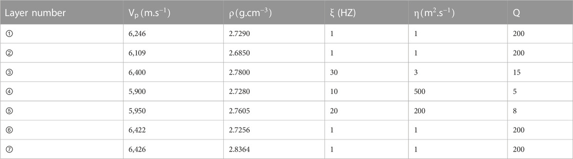
TABLE 1. Rock properties for the geological model (where, ${\mathrm{V}}_{\mathrm{p}}$ is the primary velocity, $\mathrm{\rho }$ is the density, $\mathrm{\xi }$ is the dispersion coefficient, $\mathrm{\eta }$ is the viscosity coefficient, $\mathrm{Q}$ is the attenuation coefficient).

FIGURE 4

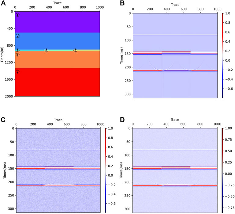
FIGURE 4. (A) Geological model. (B) The synthetic seismic record without noise. (C) The synthetic seismic record with SNR = 1 dB. (D) The synthetic seismic record with SNR = 10 dB.

When preparing the dataset, the seismic records including the stratigraphic response of layers ③, ④, and ⑤ are divided into the seismic response of the water-bearing reservoir, the gas-bearing reservoir, and the gas-water mixed reservoir, respectively. Ten seismic records with stratigraphic responses around layers ③, ④, and ⑤ are eliminated to limit the impact of distinct stratigraphic borders. Among the stratigraphic responses of each type of reservoir, 60% and 10% of the seismic records are selected randomly as training datasets and validation datasets respectively, while the remaining 30% are test datasets. In pre-processing and feature extraction, the parameter values are all adopted by our prior experiment. The pre-emphasis coefficient is 0.93, the frame length is set to 20 milliseconds (ms), and the frameshift is set the half of the frame length. Besides, Hamming window is selected because the cepstrum coefficient calculated from it is relatively stable. Then, the seismic records’ cepstrum parameters are calculated and fed into the DNN model. The DNN model in Kaldi is primarily written in C++, whereas the proposed DNN model is constructed and trained in Pytorch. When training a DNN model, the objective function is a multiclassification cross-entropy function, the optimizer uses Adam (Barakat and Bianchi, 2021), and the learning strategy is OneCycle (Smith, 2017). The training process at extremely low SNR (1 dB∼4 dB) is represented in Figure 5, while the training results with SNR greater than 4 dB are not shown since the accuracy of the training and validation datasets exceeds 98% and the loss is less than 0.1.

FIGURE 5

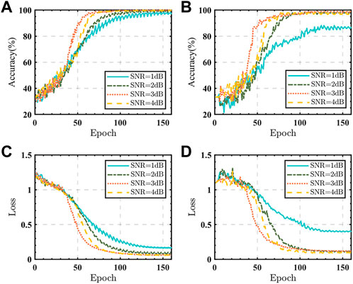
FIGURE 5. (A, B)Accuracy for training and validation sets. (C, D)Loss for training and validation sets.

When the training of the DNN model is completed, the parameter values of each DNN layer are fixed. The embedding extracted from the seismic records at the center of layers ③, ④, and ⑤ is regarded as the embedding of reservoirs in which they are located. The cosine distance between the embedding of the seismic record to be predicted and three types of reservoir embedding is calculated respectively, and the reservoir corresponding to the highest cosine distance is the predicted reservoir. When the DNN input features are Cepstrum, MFCC, and FBank, three alternative gas-bearing prediction models are generated. From the result indicated in Figures 6A, B, it can be seen that cepstrum as a feature parameter has a robust advantage over the other two features.

FIGURE 6

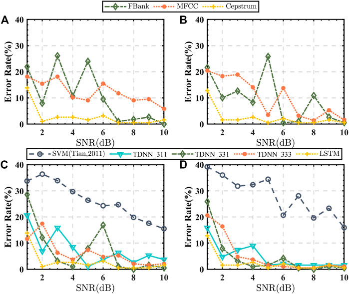
FIGURE 6. The predicted error rate of the geological model. (A) EMa with different DNN inputs. (B) EMb with different DNN inputs. (C) EMa with different architectures. (D) EMb with different architectures.

The bottom layer of the x-vector uses TDNN with context to learn the segment feature in speech recognition. The effective response time of the reservoir in the seismic record is shorter than that of the speech record, and a shorter context should be set. In order to assess the impact of contextual width, we configure the TDNN-based gas-bearing prediction models with three time-delay strategies. These three strategies, labeled as TDNN_311, TDNN_331, and TDNN_333, set the context of frames 1, frame 1∼2, and frames 1∼3 to 3 respectively, while the other layers have no delay. TDNN is implemented in the deep learning toolkit Torch by 1d-CNN because TDNN is equivalent to 1d-CNN (Daniel et al., 2018). Because the process of selecting the optimal combination from the three schemes is somewhat inefficient, we propose to replace TDNN with LSTM. To compare the improvement of the proposed method, we also compare it with previous studies (Tian and Cao, 2011), in which the absolute value of the difference between 1 and 2-order cepstral coefficients is extracted as the training samples of the support vector machine (SVM) classifier. The predicted error rate of the test samples belonging to the corresponding reserve is calculated based on different architectures respectively, which is shown in Figures 6C, D. The superior performance of LSTM shows that it may automatically learn the long-term relationships among sequences with the use of input gates, forgetting gates, output gates, and internal memory units.

4 The experiment of field

The work area is located in the Xiaoquan–Xinchang tectonic belt of the western Sichuan exploration area in China, with 150 ${km}^2$ as shown in Figure 7. This tectonic zone is mainly zonal distribution located in the Longmenshan foreland basin, one of the most important China’s natural gas-rich areas. The marine strata of this area dominated by carbonate is buried deep (about 4,000 m–7,000 m) including from Sinian to Middle Triassic. In this area, the Upper Triassic Maan Tang Formation ($T_{3}m$) and the Leikoupo Formation ($T_{2}l$) are the target layer due to massive natural gas resources. The thickness of the gas reservoir is thin, which results in minor differences in the physical parameters of the gas-bearing layer and surrounding rocks, and the poor seismic response signal makes exploration with current technologies more difficult. There are three drilled well sites in the field area, and the geological formations of Well A, Well B, and Well C are a water-bearing reservoir, a gas-bearing reservoir, and a gas-water mixed reservoir in the target layer, respectively. When the datasets are generated, the seismic record from the top weathered crust of $T_{3}m$ to the bottom of $T_2{l}_4$ (around 150 m) is intercepted as the target layer along longitudinal time. Moreover, the seismic data (about 450 records) in the lateral 300 m range around Well A, B, and C is chosen. The seismic records close to the three wells are divided into three distinct types of stratigraphic response, namely, the seismic response of the water-bearing layer, the gas-bearing layer, and the gas-water mixed layer. The training and the validation curve are represented in Figure 8.

FIGURE 7

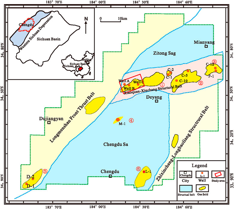
FIGURE 7. Structural diagram of the study area Cao et al. (2022).

FIGURE 8

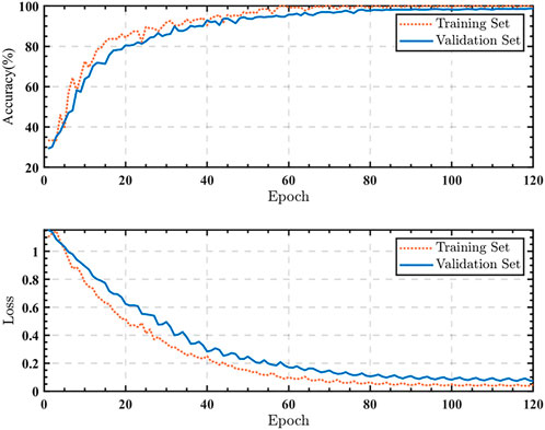
FIGURE 8. Accuracy and loss based on the field data.

After training, the seismic embeddings nearest to three wells are generated and used as the reservoir represent in which they are located. The cosine distances are calculated independently by the embeddings of the to-be-predicted seismic records and the embeddings of three reservoirs. Subsequently, the cosine score with the gas reservoir indicates the gas-bearing probability. When the Cepstrum, MFCC, and FBank are selected as input features, it shows the same phenomenon in the geological model that the error rate with Cepstrum is lower than that of the other two feature parameters in Figure 9A. Similarly, Figure 9B shows that LSTM has a moderate performance compared with the three strategies of TDNN and obvious advantages over previous SVM architectures. Further, we list the probabilities of the test samples belonging to each category with the proposed and the previous method in Figure 10. To make the comparison fairer, we normalized each probability using the formula below, where $j=\mathrm{1,2,3}$ denote the three categories of reservoirs, respectively, $P_j$ is the initial probability, and ${\dot{P}}_j$ is the normalized probability.

${\dot{P}}_j=\frac{P_j}{{\displaystyle \sum _{i=1}^3}{P}_i},j=\mathrm{1,2,3}(5)$

FIGURE 9

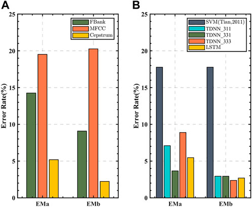
FIGURE 9. The predicted error rate of the field. (A) With different DNN inputs. (B) With different architectures.

FIGURE 10

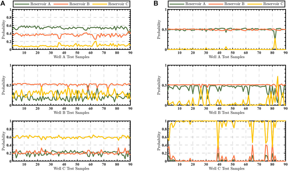
FIGURE 10. (A) The predicted probability based on EMb. (B) The predicted probability based on SVM.

To visualize the gas-bearing distribution clearly, the proposed approach is applied to the whole work area. In Figure 11, the value of the region predicted as reservoir B is equal to the cosine scoring, whereas the value of the region predicted to be reservoir A and C are set to 0 and 0.5, respectively. The prediction results based on the two embeddings show comparable gas-bearing distribution zones, while the gas-bearing region based on EMb is slightly larger which is consistent with the result in Figure 9 that fewer of the gas-bearing test samples are poorly predicted.

FIGURE 11

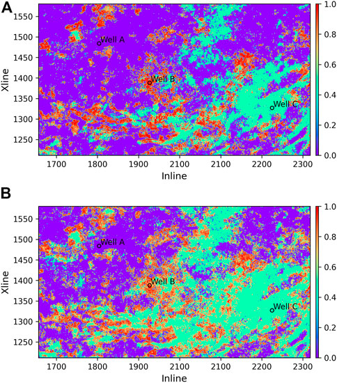
FIGURE 11. Predicted gas-bearing probability in the work area. (A) Based on EMa. (B) Based on EMb.

5 Conclusion

To deal with the difficult challenge of gas-bearing prediction in deeply buried reservoirs, this paper proposes an innovative gas-bearing prediction model based on DNN embedding. Motivated by the similarity between seismic data and acoustic data, the DNN model is designed by referring to the structure of the x-vector in speech identification, in which gas-sensitive cepstral parameters are the input, the bottom layers are LSTM networks that can learn the contextual relationship of the seismic waveforms, and the output is a DNN embedding used for similarity scoring. The validity of the proposed method was demonstrated in both generated synthetic seismic records and actual seismic data. The next study is to consider the hyperparametric assessment since the parameters in feature extraction and DNN training are mainly chosen empirically. Furthermore, data augmentation might be explored to improve predictive capabilities because data amount is the fundamental restriction of DNN.

Data availability statement

The original contributions presented in the study are included in the article/Supplementary Material, further inquiries can be directed to the corresponding author.

Author contributions

All authors listed have made a substantial, direct, and intellectual contribution to the work and approved it for publication.

Funding

The authors declare that this study received funding from the project of the SINOPEC Science and Technology Department (Grant No. P20055-6). The funder was not involved in the study design, collection, analysis, interpretation of data, the writing of this article, or the decision to submit it for publication.

This work was supported by the National Natural Science Foundation of China (Grant Nos. 42030812 and 41974160), Chengdu University of Technology Postgraduate Innovative Cultivation Program (Grant No. CDUT2022BJCX009), Technological Development for Sichuan Province (2021ZYD0030), and Natural Science Foundation of Sichuan (No. 2023NSFSC0258).

Conflict of interest

The authors declare that the research was conducted in the absence of any commercial or financial relationships that could be construed as a potential conflict of interest.

Publisher’s note

All claims expressed in this article are solely those of the authors and do not necessarily represent those of their affiliated organizations, or those of the publisher, the editors and the reviewers. Any product that may be evaluated in this article, or claim that may be made by its manufacturer, is not guaranteed or endorsed by the publisher.

References

Barakat, A., and Bianchi, P. (2021). Convergence and dynamical behavior of the adam algorithm for nonconvex stochastic optimization. Siam J. Optim. 31 (1), 244–274. doi:10.1137/19m1263443

CrossRef Full Text | Google Scholar

Cao, J., Jiang, X., Xue, Y., Tian, R., Xiang, T., and Cheng, M. (2022). The state-of-the-art techniques of hydrocarbon detection and its application in ultra-deep carbonate reservoir characterization in the Sichuan Basin, China. Front. Earth Sci. 10. doi:10.3389/feart.2022.851828

CrossRef Full Text | Google Scholar

Cao, J., Liu, S., Tian, R., Wang, X., and He, X. (2011). Seismic prediction of carbonate reservoirs in the deep of Longmenshan foreland basin. Acta Petrol. Sin. 27 (8), 2423–2434.

Google Scholar

Cao, J., Xue, Y., Tian, R., and Shu, Y. (2019). Advances in hydrocarbon detection in deep carbonate reservoirs. Geophys. Prospect. Petroleum 58 (1), 9–16.

Google Scholar

Coléou, T., Poupon, M., and Azbel, K. (2003). Unsupervised seismic facies classification: A review and comparison of techniques and implementation. Lead. Edge 22 (10), 942–953. doi:10.1190/1.1623635

CrossRef Full Text | Google Scholar

Daniel, P., Cheng, G., Yiming, W., Li, K., Xu, H., Yarmohamadi, M., et al. (2018). “Semi-orthogonal low-rank matrix factorization for deep neural networks,” in Proceedings of the Conference of the International Speech Communication Association (INTERSPEECH), Hyderabad, India, September 2018.

Google Scholar

Gao, J., Song, Z., Gui, J., and Yuan, S. (2022). Gas-bearing prediction using transfer learning and CNNs: An application to a deep tight dolomite reservoir. Ieee Geoscience Remote Sens. Lett. 19, 1–5. doi:10.1109/lgrs.2020.3035568

CrossRef Full Text | Google Scholar

Hall, M. (2006). Predicting bed thickness with cepstral decomposition. Lead. Edge. 25(2)199-204.

CrossRef Full Text | Google Scholar

Hammond, A. L. (1974). Bright spot: Better seismological indicators of gas and oil. Science 185 (4150), 515–517. doi:10.1126/science.185.4150.515

PubMed Abstract | CrossRef Full Text | Google Scholar

Hampson, D. (1991). AVO inversion, theory and practice. Lead. Edge 10 (6), 39–42. doi:10.1190/1.1436820

CrossRef Full Text | Google Scholar

He, Z., Xiong, X., and Bian, L. (2009). Numerical simulation of seismic low-frequency shadows and its application. Appl. Geophys. 5 (4), 301–306. doi:10.1007/s11770-008-0040-4

CrossRef Full Text | Google Scholar

Kumar, M., Jin-Park, T., Bishop, S., and Narayanan, S. (2020). Designing neural speaker embeddings with meta learning. https://arxiv.org/abs/2007.16196.

Google Scholar

Liu, D., Wang, X., Yang, X., Mao, H., Sacchi, M. D., and Chen, W. (2022). Accelerating seismic scattered noise attenuation in offset-vector tile domain: Application of deep learning. Geophysics 87 (5), 505–519. doi:10.1190/geo2021-0654.1

CrossRef Full Text | Google Scholar

Liao, X., Cao, J., Hu, J., You, J., Jiang, X., and Liu, Z. (2020). First arrival time identification using transfer learning with continuous wavelet transform feature images. IEEE Geoscience Remote Sens. Lett. 17 (11), 2002–2006. doi:10.1109/lgrs.2019.2955950

CrossRef Full Text | Google Scholar

Liu, D., Wang, W., Wang, X., Wang, C., Pei, J., and Chen, W. (2020). Poststack seismic data denoising based on 3-D convolutional neural network. Ieee Trans. Geoscience Remote Sens. 58 (3), 1598–1629. doi:10.1109/tgrs.2019.2947149

CrossRef Full Text | Google Scholar

Liu, Z., Cao, J., You, J., Chen, S., Lu, Y., and Zhou, P. (2021). A lithological sequence classification method with well log via SVM-assisted bi-directional GRU-CRF neural network. J. Petroleum Sci. Eng. 205, 108913. doi:10.1016/j.petrol.2021.108913

CrossRef Full Text | Google Scholar

Muda, L., Begam, M., and Elamvazuthi, I. (2010). Voice recognition algorithms using Mel frequency cepstral coefficient (MFCC) and dynamic time warping (DTW) techniques. https://arxiv.org/abs/1003.4083.

Google Scholar

Qu, X., Yan, G., Zheng, D., Fan, S., Rao, Q., and Jiang, J. (2021). A deep learning-based automatic first-arrival picking method for ultrasound sound-speed tomography. IEEE Trans. Ultrason. Ferroelectr. Freq. Control 68 (8), 2675–2686. doi:10.1109/TUFFC.2021.3074983

PubMed Abstract | CrossRef Full Text | Google Scholar

Smith, L. N. (2017). “Cyclical learning rates for training neural networks,” in Proceedings of the 17th IEEE Winter Conference on Applications of Computer Vision (WACV), Waikoloa, HI, USA, January 2017, 464–472.

CrossRef Full Text | Google Scholar

Snyder, D., Garcia-Romero, D., Povey, D., and Khudanpur, S. (2017). “Deep neural network embeddings for text-independent speaker verification,” in Proceedings of the Conference of the International Speech Communication Association, Stockholm, Sweden, August 2017.

CrossRef Full Text | Google Scholar

Snyder, D., Garcia-Romero, D., Sell, G., Povey, D., and Khudanpur, S. (2018). “X-Vectors: Robust DNN embeddings for speaker recognition,” in Proceedings of the 2018 IEEE International Conference on Acoustics, Speech and Signal Processing (ICASSP), Calgary, Canada, April 2018.

CrossRef Full Text | Google Scholar

Song, Z., Li, S., He, S., Yuan, S., and Wang, S. (2022). Gas-bearing prediction of tight sandstone reservoir using semi-supervised learning and transfer learning. IEEE Geoscience Remote Sens. Lett. 19, 1–5. doi:10.1109/lgrs.2022.3177314

CrossRef Full Text | Google Scholar

Taner, M. T., Koehler, F., and Sheriff, R. E. (1979). Complex seismic trace analysis. Geophysics 44 (6), 1041–1063. doi:10.1190/1.1440994

CrossRef Full Text | Google Scholar

Tian, R.-F., and Cao, J.-X. (2011). “Application of support vector machine method for predicting hydrocarbon in the reservoir,” in Proceedings of the 2011 International Conference on Computational and Information Sciences, Washington, DC, USA, October 2011.

CrossRef Full Text | Google Scholar

Tschannen, V., Delescluse, M., Ettrich, N., and Keuper, J. (2020). “Extracting horizon surfaces from 3D seismic data using deep learning,”, N17–N26. doi:10.1190/geo2019-0569.1Geophysics853

CrossRef Full Text | Google Scholar

Wang, F., and Chen, S. (2019). Residual learning of deep convolutional neural network for seismic random noise attenuation. IEEE Geoscience Remote Sens. Lett. 16 (8), 1314–1318. doi:10.1109/lgrs.2019.2895702

CrossRef Full Text | Google Scholar

Wang, J., Li, L., Wang, D., and Zheng, T. F. (2014). “Research on generalization property of time-varying fbank-weighted MFCC for I-vector based speaker verification,” in Proceedings of the 9th International Symposium on Chinese Spoken Language Processing 2014, Singapore, September 2014.

CrossRef Full Text | Google Scholar

Xie, T., Zheng, X.-D., and Zhang, Y. (2016). Seismic facies analysis based on linear prediction cepstrum coefficients. Chin. J. Geophysics-Chinese Ed. 59 (11), 4266–4277. doi:10.6038/cjg20161127

CrossRef Full Text | Google Scholar

Xie, T., Zheng, X., and Zhang, Y. (2017). Seismic facies analysis based on speech recognition feature parameters. Geophysics 82 (3), O23–O35. doi:10.1190/geo2016-0121.1

CrossRef Full Text | Google Scholar

Xue, Y., Cao, J., Tian, R., Du, H., and Yao, Y. (2016). Wavelet-based cepstrum decomposition of seismic data and its application in hydrocarbon detection. Geophys. Prospect. 64 (6), 1441–1453. doi:10.1111/1365-2478.12344

CrossRef Full Text | Google Scholar

Yang, J., Lin, N., Zhang, K., Zhang, C., Fu, C., Tian, G., et al. (2021). Reservoir characterization using multi-component seismic data in a novel hybrid model based on clustering and deep neural network. Nat. Resour. Res. 30 (5), 3429–3454. doi:10.1007/s11053-021-09863-z

CrossRef Full Text | Google Scholar

Zhang, K., Lin, N.-T., Yang, J.-Q., Jin, Z.-W., Li, G.-H., and Ding, R.-W. (2022). Predicting gas-bearing distribution using DNN based on multi-component seismic data: Quality evaluation using structural and fracture factors. Petroleum Sci. 19 (4), 1566–1581. doi:10.1016/j.petsci.2022.02.008

CrossRef Full Text | Google Scholar

Zheng, F., Zhang, G. L., and Song, Z. J. (2001). Comparison of different implementations of MFCC. J. Comput. Sci. Technol. 16 (6), 582–589. doi:10.1007/bf02943243

CrossRef Full Text | Google Scholar