The 3-D shallow velocity structure and sedimentary structure of 2017 Ms6.6 Jinghe earthquake source area derived from dense array observations of ambient noise

To understand the shallow structure and complex sedimentary environment of the 2017 Jinghe Ms6.6 earthquake focal area, we used one mouth of continuous sesimic data from a dense seismic array of 208 short period stations around the earthquake focal area, and applied the ambient noise tomography (ANT) method to image the three-dimensional Shear wave velocity structure at the depth less than 4 km. The shear wave velocity shown clear lateral variations and vertical variations from the surface to the deeper regions and has a tight correlation with surface geological and tectonic features in the study area. Obvious low-velocity anomalies has been presented throughout most of the Jinghe depression, whereas the Borokonu Mountains presented high-velocity anomalies. The thickness of the Cenozoic sedimentary basement in the study area is approximately 1–4 km, and the distribution of thickness is highly uneven. The crystalline basement in the study area has strong bending deformation, and the non-uniform Cenozoic sediments are related to the strong bending deformation of the crystalline basement. The Kusongmuchik piedmont fault is a high-angle thrust fault cutting through the base. There are also many medium low-angle faults, which do not penetrate the surface, which has indicated that they are in a concealed state at present. The results have provided a shallow high-resolution 3D velocity model that can be used in the simulation of strong ground motion and for evaluating potential seismic hazards.

1 Introduction

On 9 Aug 2017, the Jinghe Ms6.6 earthquake occurred in Jinghe County, Bortala Prefecture, Xinjiang Uygur Autonomous Region (Figure 1). The epicenter was located at 44.27°N and 82.89°E, and the depth was 11 km as measured by China Earthquake Networks Center. Near the epicenter, near the epicenter strong tremors can be felt. Less than a day after the earthquake, a total of 11 aftershocks occurred with M ≥ 3, which affected 33 towns. 32 people were injured, and 142 houses collapsed (Jin et al., 2019; He et al., 2020). One year later, one Ms5.4 earthquake occurred 30 km away to the southwest of the Jinghe Ms6.6 earthquake. Many earthquakes have occurred in this area over a relatively short time, which has resulted in a strong research focus on the seismogenic mechanisms in this area.

FIGURE 1

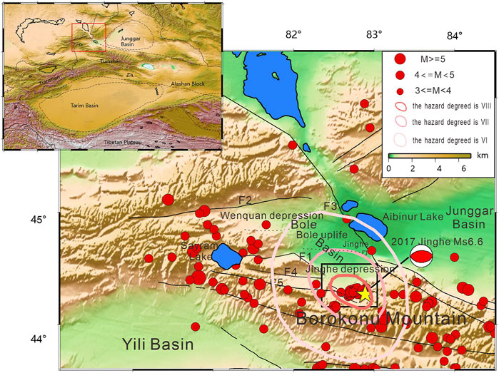
FIGURE 1. Topographic and seismicity maps of the study area.

Xinjiang is located on the Eurasian seismic belt, where there are many large faults, and earthquakes are active. However, given the wide area, poor surface conditions, and sparse observation stations in Xinjiang, so far, there has been relatively little research on the crust structure in this area. In particular, there is relatively little understanding of the deep and shallow structure of active faults in this area. This affects the understanding of the background around the mechanisms of earthquake generation and their dynamics. After the earthquake, the regional arrays were used to carry out seismic tomography, seismic relocation, and geometric analysis of seismogenic faults in this area (Fu and Wang, 2020; He et al., 2020). However, given the sparse distribution and low resolution of the array, their understanding of the deep seismogenic background in this area has been relatively limited.

The deep crustal structure is closely related to the development of earthquakes, and the structure of the shallow crust is directly related to earthquake disasters. Areas with extensive structural changes such as fault zones are often those with the serious earthquake disasters. Considering that sedimentary structures can amplify seismic signals, it is also likely to increase earthquake damage (Li et al., 2020). Therefore, in the study of earthquake disaster prediction, we should not only pay attention to information on faults but also pay attention to the sedimentary structure of the basin. The Jinghe area is located on thick sedimentary structures, and to reduce the risk of earthquake disasters, it is important to investigate the deep structured and seismogenic background of the fault, as well as determine the sedimentary structure. Studying the sedimentary structure is also play a key role in exploring resource and energy distribution in the shallow crust. This is of considerable importance in the study of the sedimentary environment related to faults, strong earthquake ground motion, and disaster risk prediction.

In recent years, the high-frequency surface wave signal has been obtained using continuous ambient noise data based on the dense seismic array. It is more sensitive to the shallow velocity structure and small-scale ambient noise tomography has been widely used in cities, volcanic activities, metal mines, and other areas (Lin et al., 2013; Fang et al., 2015; Luo et al., 2015; Li et al., 2016; Zhou et al., 2018; Gu et al., 2019; Zellmer et al., 2019; Zulfakriza et al., 2020). A dense seismic array with 208 three component short period seismometers was deployed on 5 July 2018. The range is about 50 km × 50 km with the station spacing being 0.5–5 km (Figure 2). In this study, we determined the 0–4 km three-dimensional (3D) shear wave velocity in the Jinghe area by inverting 1–5 s period dispersions using direct surface wave tomography (Fang et al., 2015).

FIGURE 2

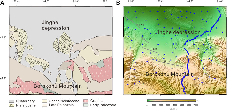
FIGURE 2. (A) Geological map of study area; (B) The stations used in this study are shown in the red rectangle in (A), F1 is the Kusongmuchik piedmont fault.

2 Geological background

The study area was located in the southern of the Bole Basin and the contact part of the Boluokonu Mountain and Kogurqin Mountain (Figure 2A), which form part of the Sayram micro block. The Bole basin is a composite basin of the Upper Paleozoic and Mesozoic Cenozoic, and the Devonian system directly covers the Mesoproterozoic metamorphic rocks. The basin comprises three secondary structures, the Wenquan Depression, Bole Uplift, and the Jinghe Depression. According to the analysis of field outcrops, seismic and drilling data, Devonian, Carboniferous, Permian, Jurassic, Paleogene, Neogene, and Quaternary strata are developed in the basin. The Paleozoic strata is relatively thick, and the Mesozoic Cenozoic strata are relatively thin. Devonian and Carboniferous strata are widely distributed in this area. The Permian system is developed in the west of the Bole uplift, and the entire Triassic system is missing. The Jurassic system is only distributed to the northwest of the Wenquan Depression, and the Tertiary and Quaternary systems are distributed throughout the basin (Sun et al., 1997; Zhang et al., 2017a; Zhang et al., 2017b).

The Borokonu and Kogurqin mountain belts are located in the northern branch of the Western Tianshan Mountains and the northern margin of the Yili Basin. They are characterized by a Paleozoic active continental margin superimposed onto the Precambrian metamorphic crystalline basement (Gao et al., 2009). The Boluoli island arc belt is located in the south and the nappe structure is located in the north. Most of the strata exposures on the Boluokonu Mountain are from the Proterozoic and Paleozoic (Wang et al., 2013), and most of the strata exposed on Kogurqin Mountain are Proterozoic.

The Jinghe earthquake occurred near the eastern section of the Kusongmuchik piedmont fault at the north edge of the Bolokonou Mountain, to the north of Tianshan Mountain, and at the southwest end of the Junggar Basin (Figure 1). The study area was located in the thrust fold tectonic active belt between the Junggar plate and the Tianshan plate. The Kusongmuchick piedmont fault is a newly active fault that has developed on the fold reverse fault zone at the front edge of the Tianshan nappe (Chen et al., 2007). The Kusongmuchik piedmont fault is a Holocene Active fault (Chen et al., 2007), which is a dextral reverse fault that is EW trending. The fault is a boundary fault and regionally active fault located on the north edge of the west end of North Tianshan. According to its activity trends, it is divided into the east, middle, and west segments. Chen et al. (2007) obtained the stratigraphic and structural data from the area through field investigation. It was found that the eastern section of the Kusongmuchick piedmont fault is approximately 50 km long, predominantly composed of four fault oblique columns with a strike of 280°–290°, a length of 9–13 km, with a dip to the south (Figure 2 marked as f2-1, f2-2, f2-3, and f2-4), the dip angle of 40°–60°. Faults and folds have developed in the area where the fault is located, and there is a high level of tectonic activity.

3 Data and methods

From May to July 2018, the Geophysical Exploration Center, China Earthquake Administration deployed a 150 km long linear dense array using the Jinghe County, Nileke County, and Gongliu County of Xinjiang with a NE–SW trend, with an average station spacing of approximately 500 m, comprising 115 stations. The linear array was located through the epicenter area of the Jinghe Ms6.6 earthquake. Meanwhile, a plane dense array was deployed around the epicenter area, with these detector stations spanning an area of 44.16°N–44.54°N and 82.37°–83.04°E, with a total of 115 stations spaced approximately 4 km apart. The original data sampling rate was 200 Hz. The observation instruments used were short-period portable digital seismometers and the corner frequency of the instrument was 5 s. In this study, we used the continuous ambient noise data recorded by the plane dense array and 93 stations of a linear dense array inside the planar array with a total of 208 stations (Figure 2B). This was undertaken to obtain a high-resolution image of the shallow structure beneath the region of the Jinghe Ms6.6 earthquake area. The main fault in the study area was the eastern part of the Kusongmuqike piedmont fault, which is composed of four faults. The trend was 280°–290°, at approximately 50 km, with a dip to the south (Figure 2B marked as F1-1, F1-2, F1-3, F1-4).

The empirical Green’s function between station pairs could be derived from the noise cross-correlation function stack over relatively long timescales. In this study, we used the vertical component data to calculate the cross-correlation function between stations and extract the Rayleigh surface wave signal. Before using noise data to calculate the cross-correlation function, it is necessary to preprocess single station data, which follows the data processing process for the noise cross-correlation standard (Bensen et al., 2007). The data was reduced to 1 day in length and the original 200 Hz data was downsampled to 50 Hz. We then removed the mean and the trend of the data and band-pass filtered the data in the 0.1–10 s frequency band. To reduce the effect of earthquake signals, we performed spectral whitening and temporal normalization of the data. We performed cross-correlation to obtain the time domain cross-correlation function (CF) for Station Pairs A and B for each set of daily data with a lag time from −100 to 100 s. After preprocessing was complete, the cross-correlation between all the stations could be calculated. All the daily CFs from each station pair was stacked together linearly. A total of 21,528 cross-correlations were obtained in this study. Figure 3 shows an example of noise correlation functions of the vertical–vertical component, based on the long observation time. The CFs of the signal-to-noise ratio (SNR) was relatively high, and we could observe clear surface wave signals in the positive and negative time parts. The surface wave signal was clearly in line with the positive and negative time components. Although the amplitude information was different, the time of arrival of the positive and negative surface waves was consistent.

FIGURE 3

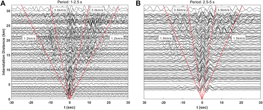
FIGURE 3. (A) A record section of CFs in a period band of 1–2.5 s; (B) A record section of CFs in a period band of 2.5–5 s.

To improve the cross-correlation SNR, we linearly stacked the positive time and negative time components of Empirical Green’s function. The group velocity dispersion curve of the Rayleigh surface wave was automatically extracted using the image analysis method of Yao et al. (2006); Yao et al. (2011). According to the relationship between station spacing and wavelength, we extracted the dispersion curve of 1–5 s, with a sampling interval of 0.1 s. We required the interstation distance to be at least double the wavelength to approximately satisfy the far field approximation of surface wave propagation (Yao et al., 2010), and the SNR ≥5. Using this program, a reliable reference dispersion curve was needed to function. Therefore, 200 dispersion curves were manually identified, and the reference dispersion curve was calculated using these data. A total of 15,700 dispersion curves were extracted using the manually selected dispersion calculation. We controlled the quality of the automatically extracted dispersion curve. According to the reference dispersion curve, the maximum slope of the dispersion curve was 0.5. Therefore, we retained data with a group velocity difference of two adjacent periods less than or equal to 0.05 km/s and then deleted the dispersion curve with less than five points. Therefore, the quality control of the dispersion curve was completed. A total of 5,724 high-quality dispersion curves were retained. According to the dispersion data extracted, statistical information on dispersion quantity over different periods was obtained (Figure 4). In 1–2.8 s with the increase in duration, the number of dispersion increased, and the most number of dispersions occurred over 2.8 s at nearly 3,000. After 2.8 s, with the increase in duration, the number of dispersions gradually decreased to about 1,000.

FIGURE 4

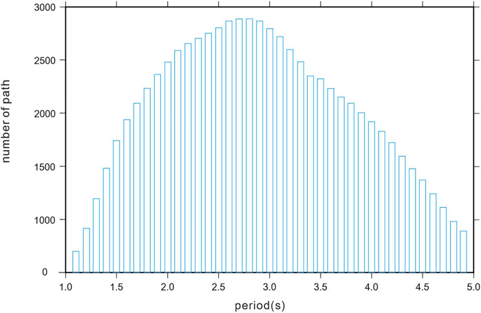
FIGURE 4. The number dispersion at different period.

4 Results

4.1 Inversion method

In this study, we used the direct surface wave tomography method with period-dependent ray tracing method to invert all the dispersive travel-time data simultaneously for the 3D subsurface shear-velocity structure (Fang et al., 2015). This method can be used to avoid the intermediate steps of inversion for phase or group velocity maps and considers ray bending effects on surface-wave tomography in the complex medium. For the forward problem, the fast-matching method was used to compute the surface wave travel times and ray paths between receivers and sources for each period (Rawlinson et al., 2004). The travel-time perturbation at the angular frequency ω concerning a reference model for the path is given by Fang et al. (2015).

$\delta t_i\left(\omega \right)=t_i^{obs}\left(\omega \right)-t_i\left(\mathrm{\omega }\right)\approx -{\displaystyle \sum _{k=1}^K}{v}_{ik}\frac{\delta C_k\left(\omega \right)}{C_k^2\left(\omega \right)}(1)$

in which ${\mathrm{t}}_{\mathrm{i}}^{\mathrm{o}\mathrm{b}\mathrm{s}}\left(\mathrm{\omega }\right)$ is the observed surface wave travel time, ${\mathrm{t}}_{\mathrm{i}}\left(\mathrm{\omega }\right)$ is the travel time calculated from a reference model that can be updated in the inversion, and is the bilinear interpolation coefficients along the ray path associated with the i th travel time data and the phase (or group) velocity ${\mathrm{C}}_{\mathrm{k}}\left(\mathrm{\omega }\right)$ and its perturbation.

$\mathrm{\delta }{\mathrm{C}}_{\mathrm{k}}\left(\mathrm{\omega }\right)$ of the k th 2D surface grid point at the angular frequency ω. Using the 1D depth kernel of Rayleigh wave phase or group velocity data to compressional velocity (a), shear velocity (ß), and density (ρ) at each surface grid node, we can rewrite Eq. 1 as

$\mathrm{\delta }{t}_i\left(\omega \right)={\left.{\displaystyle \sum _{k=1}^k}\left(-\frac{v_{ik}}{C_k^2\left(\omega \right)}\right){\displaystyle \sum _{j=1}^J}\left[R_a\left(Z_j\right)\frac{\partial C_k\left(\omega \right)}{\partial a_k\left(z_j\right)}+R_{\rho }\left(z_j\right)\frac{\partial C_k\left(\omega \right)}{\partial {\rho }_k\left(z_j\right)}+\frac{\partial C_k\left(\omega \right)}{\partial {\beta }_k\left(z_j\right)}\right]\right|}_{{\mathrm{\Theta }}_k}\delta {\beta }_k\left(z_j\right)={\displaystyle \sum _{l=1}^M}{G}_{il}{m}_l(2)$

In which ${\mathrm{\theta }}_{\mathrm{k}}$ represents the 1D reference model at the kth surface grid point on the surface, ${\mathrm{\alpha }}_{\mathrm{k}}\left({\mathrm{z}}_{\mathrm{j}}\right)$, ${\mathrm{\beta }}_{\mathrm{k}}\left({\mathrm{z}}_{\mathrm{j}}\right)$, and ${\mathrm{\rho }}_{\mathrm{k}}\left({\mathrm{z}}_{\mathrm{j}}\right)$ are the compression velocity, shear velocity, and mass density at the j th depth grid node, respectively. $R_{\alpha }^{\prime }$ and $R_{\rho }^{\prime }$ are the scaling factor, J is the number of grid points in the depth direction, and the number of total grid points of the 3D model is M = K ╳ J. We can write (2) as

$\mathrm{d}=\mathrm{G}\mathrm{m}(3)$

In which d is the travel time residual, G is the data sensitivity matrix, and M is the model parameter. In the inversion problem, the loss function needs to be minimized to solve formula (3), we can obtain (4)

$\mathrm{\Phi }\left(\mathrm{m}\right)=‖d-{GM‖}_2^2+\mathrm{\lambda }‖{LM‖}_2^2(4)$

Where the first term on the right-hand side gives the $l_2$-norm data misfit and the second term denotes the $l_2$-norm model regularization term and the second term is the model regularization term. L is the model smoothing factor; λ is the weight factor of data fitting and model regularization. Therefore, the solution m of formula (3) is

$\stackrel{\sim }{\mathrm{m}}={\left(G^T\mathrm{G}+\mathrm{\lambda }{L}^T\mathrm{L}\right)}^{-1}{G}^{T}d(5)$

Therefore, the inversion problem is transformed into the least square problem in linear inversion (Paige and Saimders, 1982).

4.2 3D model and sensitive kernel

We used direct inversion of 3D S-wave velocity imaging based on independent period ray tracing (Fang et al., 2015) to simultaneously all the dispersions to obtain the S-wave velocity structure of the study area. This includes inversion without the intermediate step of phase- or group-velocity maps and avoids the effect of bending off the great-circle ray in a complex medium.

We used the 1D velocity model of the Tianshan area obtained by Shao. (1996) as the initial velocity model (Figure 5A blue line). The inversion depth was 0–7 km, and there were 14 layers along the depth direction. We calculated the average dispersion curve for all the group dispersion curves. The linear inversion program (Herrman and Ammon, 2004) was used to invert the average dispersion curve to obtain the 1D shear velocity structure (Figure 5A red line). We used the 1D model (Figure 5A red line) to construct the initial three-dimensional inversion model and set the grid spacing to 0.02°, which was equivalent to 30 × 50 = 1,500 horizontal grid points.

FIGURE 5

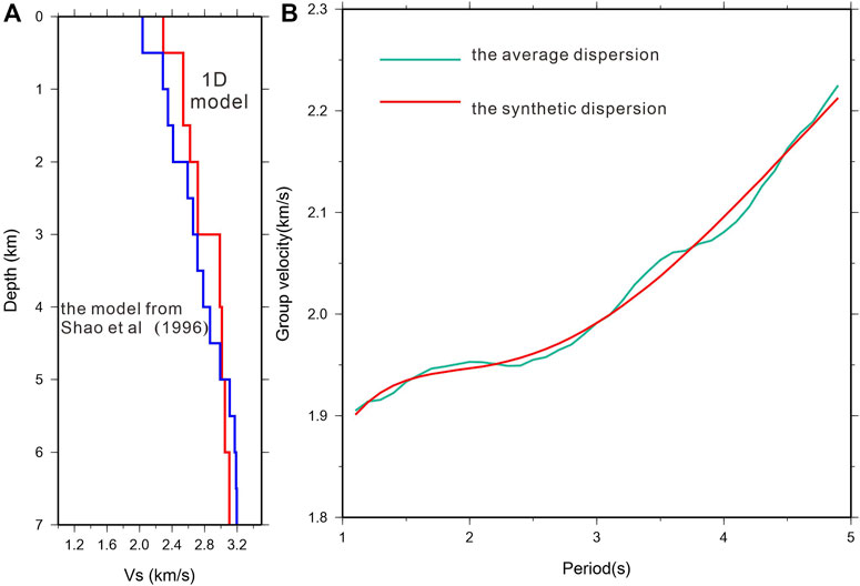
FIGURE 5. (A) The initial model from Shao et al. (1996) (blue line), the 1-D model derived from inverting the measured average group velocity dispersion. (B) The green line is the observed average dispersion curve; the red line indicates the dispersion curve obtained by forward calculation using the 1-D average velocity model in FigureA.

We calculated the depth-sensitive kernel function of group velocity with a period of 1–5 s to the S-wave velocity using the 1D model (Figure 5A red line). Figure 6 shows that the maximum sensitive depth of the different Rayleigh waves is approximately 1/2λ (wavelength). According to the sensitive kernel function, the group velocity of 0.5–5 s was mainly sensitive to the depth range of 0–5 km.

FIGURE 6

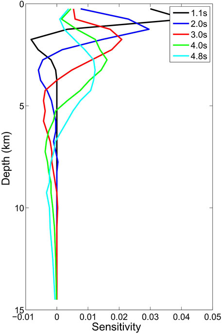
FIGURE 6. Depth sensitivity kernels for group velocity at four periods: 1.1, 2.0, 3.0, 4.0, and 4.8 s.

4.3 Path coverage and resolution

The resolution of surface wave tomography depended primarily on the coverage and azimuthal distribution of the path. The denser the ray path coverage, the higher the resolution; on the contrary, the thinner the path coverage, the lower the resolution. Based on the final inversion, we obtained the path coverage for the group velocity for all periods (Figure 7). The distribution of the ray paths for each period was similar, and the path density in the northwest of the study area was lower than the southeast, due to uneven distribution of stations. With the period increases, the ray coverage density decreases.

FIGURE 7

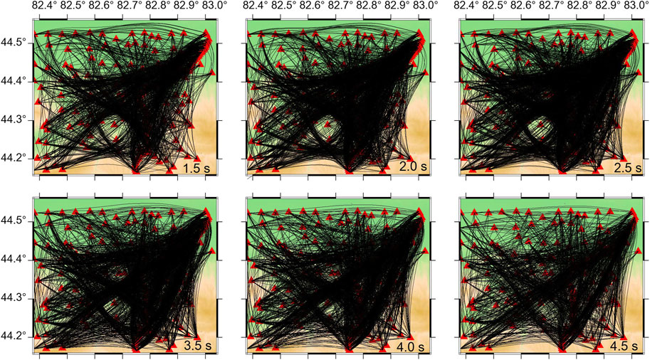
FIGURE 7. The ray paths obtained from the final 3-D model (see Figure 9) at four periods using the fast marching method: 1.5, 2.0, 2.5, 3.5, 4.0, and 4.5 s. The black lines represent the ray paths and the red triangles represent the stations.

We used the checkerboard test to determine which part of the study area should be sufficiently well resolved by our data to justify the inversion of group velocity dispersion curves for the shear wave velocity depth profiles. The checkerboard test uses synthetic data generated on a “checkerboard” velocity structure (Figures 8A–C), using the same station pairs as the observed data. Areas, where the inversion is in line with the original checkerboard pattern, are considered well-resolved. We tried various checkerboard cell sizes of 4.5 $\times$ 4.5 km, 6 $\times$ 6 km, and 7.5 $\times$ 7.5 km throughout 2 s to determine which sizes are well resolved in the study area (Figures 8D–F). Figure 8 shows that the checkerboard test can recover the initial velocity model at 6 $\times$ 6 km cell size (Figures 8B, E). The checkerboard test at 6 $\times$ 6 km can be recovered effectively in most parts of the study area and was only poor in marginal areas.

FIGURE 8

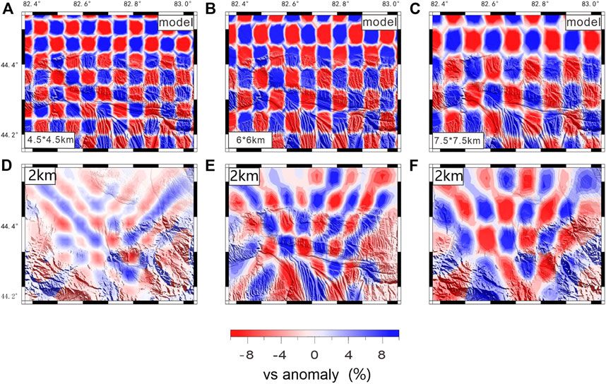
FIGURE 8. The checkboard test by using grid 6*4.5 km, 6*6 km, 7.5*7.5 km for 2 km. (A–C) show the initial velocity model and (D–F) show the recovery model.

To determine the resolution of the 3D shear velocity structures, we used the checkerboard resolution test. The initial velocity model of the checkerboard is the same as the real inversion velocity model. The grid is divided into and the disturbance volume is 27%. Figure 9 shows the checkerboard test results at depths of 0.5, 1.0, 1.5, 2.0, 2.5, and 3.5 km. The resolution is related to the path coverage and, in general. There is dense path coverage; the resolution of the checkerboard resolution test was relatively high. At the edge of the study area, where the path coverage becomes sparse, the resolution became relatively low. At a depth of 0.5–2 km, the ray path coverage is relatively dense, and the checkerboard recovery was better. With the increase in depth, the ray path gradually became sparse. The restoration of the checkerboard became worse at the edge of the study area, but it could be restored in the center area. We also obtained the test results of the depth along the longitudinal and latitudinal directions (Figure 10). The grid size of the depth checkerboard test setup gradually increased with increasing depth, with the grid size being 6 km in the horizontal direction. In terms of depth, the shallowest was 600 m with increasing crustal depth, and the grid size gradually increased to 1,500 m. The results have shown that the checkerboard recovery has occurred more successfully in the shallow section with relatively dense dispersion curve coverage. With increasing depth, the dispersion curve coverage was lower, and the checkerboard recovery gradually became less successful in the edge area.

FIGURE 9

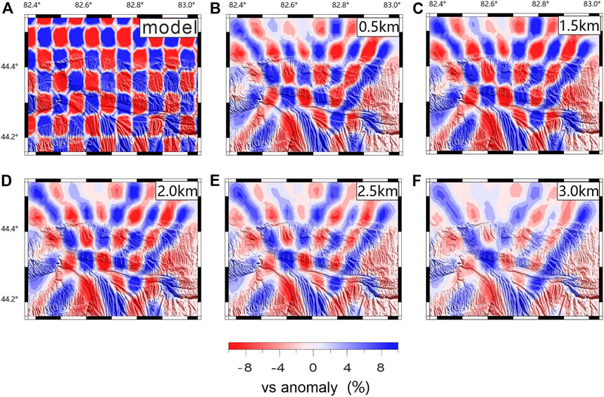
FIGURE 9. Checkerboard resolution tests of the inversion results: (A) Checkerboard test model, (B–F) different depth of horizontal checkerboard recovery.

FIGURE 10

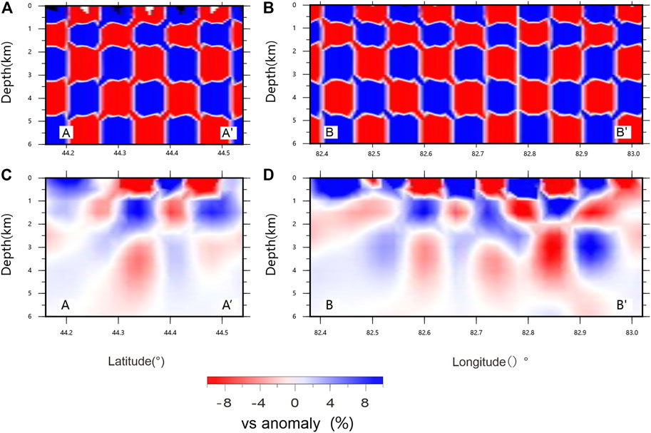
FIGURE 10. Vertical checkerboard test; the location of the profiles show in Figure 12. (A, B) are the checkboard theoretical model, (C, D) are the vertical chessboard recovery in longitude direction (D) vertical chessboard recovery in latitude direction.

4.4 3D shear velocity structure

We used all the group velocity dispersions to invert the 3D near-surface shear velocity structure. The standard deviation of travel time residuals decreased from approximately 1.74 s to approximately 1.638 s (10th iteration, see Figure 11). The last travel time residuals were highly concentrated around 0 s (Figure 11, illustration).

FIGURE 11

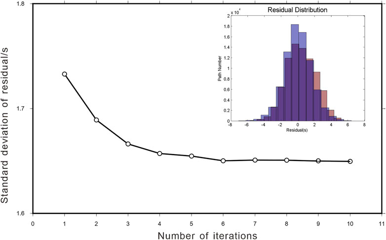
FIGURE 11. Variation of the standard deviation of surface wave travel time residuals with the number of iterations. The histogram of travel time residuals before iteration (red) and after 10 iterations (blue).

Figure 12 shows the shear velocity maps at six depths, that is, 0.5, 1.0, 1.5, 2.0, 2.5, and 3.5 km. The shear velocity maps have shown clear lateral and vertical variations which correlate closely with the main geological structures and tectonic units in the study regions.

FIGURE 12

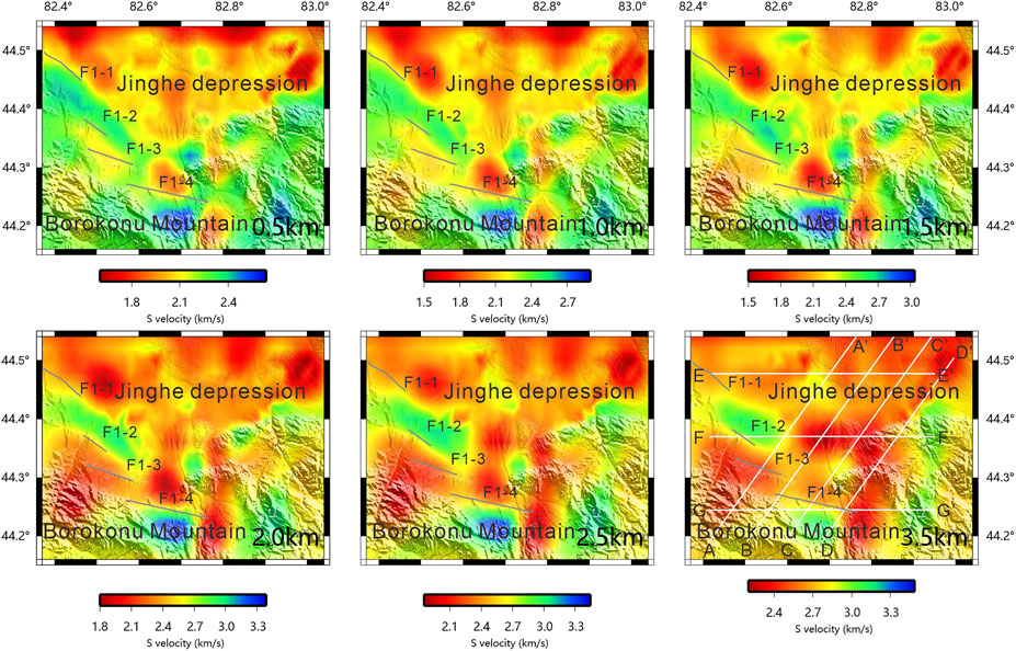
FIGURE 12. S wave velocity distribution at different depths: depth is 0.5, 1.5, 2.5, and 3.5 km.

The velocity structure characteristics of 0.5, 1 km, and 1.5 km are similar. The Jinghe depression has shown low shear wave velocity; in the valley and the area where the river passes of the Borokonu Mountain shows low velocity, whereas the other region of the Borokonu Mountain has shown high velocity. From near the surface to the deep regions, most of the Jinghe depression with thicker sediments is characterized by low shear wave velocity. Meanwhile, Borokonu Mountain, with its exposed bedrock, is characterized by higher velocities. The location is in the eastern part of Kusongmuqike Piedmont Fault (F1-1) which is the boundary of high and low velocity. The surrounding areas of F1-2 and F1-3 are characterized by high velocity, while the surrounding areas of F1-4 are characterized by low velocity. The results for the shear wave velocity structure have shown a strong correspondence with the geological features of the study area. It indicates that the velocity distribution characteristics in the study area are mainly controlled by regional structures.

Compared with the shallow structure, the velocity structure of 2, 2.5, and 3.5 km are different, with the Jinghe depression still showing a large area of low velocity. In the Borokonu Mountain, the distribution range of low velocity gradually increases, while the distribution range of high velocity gradually decreases. The eastern part of the Songmuqike Piedmont Fault has a high-velocity distribution, but the range of high speed gradually decreases with increasing depth.

We have obtained several profiles, the profiles of AA’, BB’, CC’, and DD’ (Figure 13) are near-vertical to the Kusongmuqike piedmont fault with a NE trend. The EE’, FF’, and GG’ are three profiles at the latitudes of 44.22 °N, 44.36 °N, and 44.48 °N. From the four profiles of AA’, BB’, CC’, and DD’ (Figure 13), the velocity of the Jinghe depression of the shallow 0–2 km depth range is substantially lower than that of the Boluokonu Mountain. In the range of 2–4 km, the distribution of velocity is relatively complex. From the southwest side to the northeast side, it is characterized by alternating high and low velocities. The EE’s profile along the latitudinal direction traverses the Jinghe depression, showing a low-velocity structure, and the velocity on the west side of the profile is considerably lower than that on the east side. The FF’ profile passes through the Boluokonu Mountain, the Jinghe depression, and the Boluokonu Mountain, which has high velocity in the east and west of the profile and low velocity in the middle of the profile. The GG' profile traverses the Borokonou Mountain and has high velocity, but near the Kusongmuqike piedmont fault, it has low velocity.

FIGURE 13

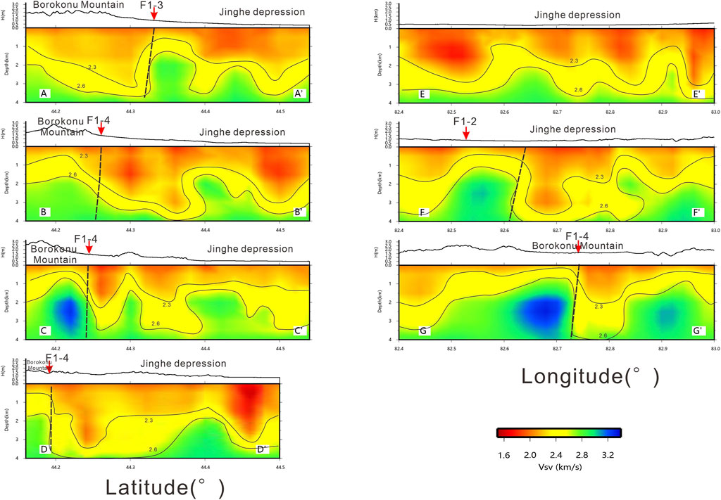
FIGURE 13. The velocity distribution of AA’, BB’, CC’, DD’, EE’, FF’, and GG’.

5 Discussion

The Bole Basin is an intermountain in the Selimu micro block in the western section of the Tianshan Mountains with a Precambrian base, which may be a basin covered by nappes (Sun et al., 1997; Wang et al., 2013; Zhang et al., 2017a). In the early Paleozoic, the northern Tianshan Junggar Ocean in the north of the Selimu micro block began to subduct southward, and the Alatao, Bizhentao, and Kogurqin Mountains began to form. During this period, the Selimu micro block was under the background of uplift. The Bole uplift in the center of the basin divided the basin into Wenquan and Jinghe depressions with the influence of mountain uplift. At this time, the structural styles of two depressions with one uplift were basically formed. In the early Permian, the lake basin declined and generally accepted sedimentation. In addition to Bole uplift, sedimentary structures of deep lake facies and volcanic eruption facies in the upper Permian were formed. From the end of Hercynian period to Indosinian period, the lake basin was uplifted and suffered weathering and denudation, which made the basin generally lack part of the Triassic and Lower Jurassic sediments in this period. At the same time, because the basin was still subject to the uplift and compression of mountains in this period, the tectonic framework of two depressions with one uplift developed by compressional and torsional reverse faults was more obvious. In the middle Yanshan period, the basin declined and entered a stable sedimentary stage; in the late Yanshan period, the basin was always in the uplift stage, and the original subsidence center lifted the fold to form the piedmont fold of Jurassic strata, while the upper Jurassic and Cretaceous sediments were generally absent. During the Himalayan period (the Tianshan Mountains were uplifted again), the orogeny was strong, the basin declined, and huge thickness of Cenozoic alluvial fan and molasse facies debris was deposited. Due to the uplift of the three sides of the mountain, fold structures and contemporaneous and associated faults were well developed, forming the current complex structural pattern (Sun et al., 1997; Wang et al., 2013; Wang et al., 2000; Gao et al., 2016; Zhang et al., 2017a; Zhang et al., 2017b).

Considering that there has been little research in the study region, we found that the Piedmont basement of the North Tianshan Mountains could be divided into two layers according to the results of the geoscience large section (report) basement crossing the three mountains and two basins in the north and south of Xinjiang approximately 200 km away from the east of the study area. The upper layer is composed of lower-velocity Cenozoic sediments; the next layer is composed of Paleozoic sediments with high velocity. According to the result of Wang et al. (2000), the Late Cenozoic sedimentary thickness is approximately 2–4 km, and the P-wave velocity is 3.5–4 km/s. Meanwhile, according to the wave velocity ratio of 1.77 in this area, the S-wave velocity calculated was approximately 1.4–2.3 km/s. This corresponds closely to the S-wave velocity structure obtained from inversion. Therefore, the thickness of the Late Cenozoic sedimentary in this area is calibrated according to the velocity of 2.3 km/s. The thickness of the late Cenozoic sedimentary is shown in Figure 14. The section shows that the thickness of the Late Cenozoic sedimentary basement in the study area is about 1–4 km, that the Late Cenozoic sedimentary basement of Borokonu Mountain is thin, and of Jinghe Depression is thicker. However, there are also pronounced differences in some areas. Sections AA’, BB’, CC’, and DD’ are strongly bent and deformed.

FIGURE 14

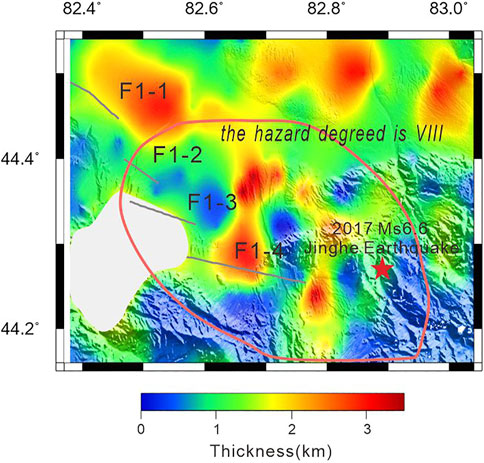
FIGURE 14. The distribution of Cenozoic sedimentary thickness. The red star is the epicenter of the 2017 Ms6.6 Jinghe Earthquake.

According to the evolutionary structure of the area, the Cenozoic sediments covered the Mesozoic strata. In the late Jurassic, the south–north compression activity of the basin was strengthened, the basement was uplifted, and the basin was deposited, resulting in substantial shrinkage of the basin. The profile map has shown that the strata under the Cenozoic sediments have shown strong fold deformation, indicating that the Jinghe Depression was strongly compressed during this period. This result is in line with those of Qi et al. (2008) on tectonic deformation within the transitional belt between Junggar Basin and the northern Tianshan Mountain. Under the influence of the uplift of the Qinghai–Tibet Plateau, the compression in the near north–south region has been strengthened, and then caused the uplift of the North Tianshan Mountains. Based on the existing faults and weak layers in the sedimentary basin cover, fold structures related to the basement involving thrust faults were formed in the Basin-Mountain transition zone of Junggar, North Tianshan. Our results may also indicate that Jinghe Depression is located in the transitional zone between the Junggar Basin and the Tianshan Mountains. From the Cretaceous to the Paleogene, Junggar Basin continued to develop under the action of isostatic curvature of the crust, and the faulting activity of the basin and its edge weakened. In the Neogene, the Tianshan Mountains began to uplift because of the collision between the Indian plate and the Eurasian plate. The Jinghe Depression formed a piedmont depression that received a substantial thickness of sediments, and the basin fillings were folded and deformed in the late sedimentation period (Wang et al., 2000). This result is also consistent with the thicker Cenozoic sedimentary facies in this area (Figure 12). Stratum bending features are also found in the EE’, FF’, and GG’ profiles, which may indicate that the study area is not only compressed by north–south compressive stress, but also by east–west stress from Kazakhstan on the west side. There are also a series of nappe structures comprising north-dipping faults from north to south on the northern edge of the Bole Basin, indicating that the area has also been compressed from the Alatao Mountain (Sun et al., 1997; Zhang et al., 2017b). This may also indicate differences between the study region and the Basin-Mountain transition zone of Junggar, North Tianshan.

The Basin-Mountain transition zone of Junggar, North Tianshan has developed thrust faults while forming a fold structure from north–south compression. The main fault is a high-angle thrust fault inclined to the basin, and a series of branch thrust faults have developed in the footwall (Qi et al., 2008). The AA’, BB’, DD’, FF’, and GG’ vertical profiles have shown that there is a substantial difference in velocity on both sides of the fault. The fault is a high-angle thrust fault, which can continue to a depth of 4 km, which indicates that the fault is a fault break-through the basement. In the area of the Piedmont basement fold, there are many medium low-angle faults, which do not break-through the surface, which may indicate that they are in a concealed state at present.

Our results have shown that the thickness of the Cenozoic sediments in Jinghe Depression is approximately 1–4 km, as we know the thicker sediments may contain rich natural resources. Zhang et al. (2017a) concluded that the southwest of Jinghe Depression is an important oil exploration area through the evaluation of the geological conditions of Bole Basin. According to its low speed in the sedimentary basin, when the earthquake propagates to the sedimentary layer, the signal is significantly amplified, which can cause greater seismic damage. After the Jinghe 6.6 earthquake on 9 August 2017, the Xinjiang Earthquake Administration released the hazard degree of the Jinghe M6.6 earthquake (Xinjiang Earthquake Administration, 2018). The hazard degree of the extreme seismic region was VIII, with an area of 979 km², a long axis of 44 km, and a short axis of 29 km. Meanwhile, many Level VIIII abnormal points were also found, and Urumqi more than 400 km away, also felt the earthquake. The area of the VIII degree area of the Jinghe earthquake is wider compared to other areas, such as the area of hazard with a degree of VIII from the Jinggu earthquake of M6.6 on 7 October 2014, is 400 km² (China Earthquake Administration, 2017a), the area of hazard with a degree of VIII from the Jiuzhaigou earthquake of M7.0 of 8 August 2017, is 778 km² (China Earthquake Administration, 2017b), the area of hazard with a degree of VIII of the Milin earthquake of M6.9 of 18 November 2017, is 310 km² (China Earthquake Administration, 2014), the area of hazard with a degree of VIII from the Luding M6.8 earthquake on 5 September 2022, is 505 km² (Ministry of Emergency management of the People’s Republic of China, 2022). Figure 14 shows that the area of the VIII degree of hazard in the Jinghe Depression is substantially larger than that of the Borokonu Mountain. The Jinghe earthquake caused a wider range of disasters that may have been related to the huge Cenozoic sediments in this area. Although Xinjiang is sparsely populated because it is close to the Eurasian seismic belt, the area is seismically active and has a background of earthquakes above magnitude 6.0, so it is urgent to address seismic fortification in this area.

6 Conclusion

Based on the ambient noise data obtained from 208 dense stations deployed in the Jinghe earthquake area, the basic Rayleigh surface wave group velocity dispersion curve with a period of 1–5 s was extracted. We then used the direct surface wave tomographic method with period-dependent ray tracing constrained to invert group dispersion travel time data simultaneously for 3-D shear wave velocity structure. The shear wave velocity model results from 0.5–4 km depths have shown the distribution of buried faults under the study area; the velocity structure anomaly has a strong correlation with regional fault structures and has a strong correlation with the complex sedimentary structure near the surface. From near the surface to the deeper regions, most of the Jinghe depression with thicker sediments is characterized by low shear wave velocity. Meanwhile, the Borokonu Mountains, with their exposed bedrock, are characterized by higher velocities. The thickness of the Cenozoic sedimentary basement in the study area is approximately 1–4 km, and the distribution is highly uneven. The crystalline basement in the study area has strong bending deformation, and the non-uniform Cenozoic sediments are related to the strong bending deformation of the crystalline basement. There is a substantial difference in velocity on both sides of the fault, and the fault can continue to a depth of 4 km, which may indicate that the fault is a fault cutting through the basement. In the area of the Piedmont basement fold, there are many medium low-angle faults, which do not break-through the surface. This may indicate that they are in a concealed state at present. The results have provided a shallow high-resolution 3D velocity model that can be used in the simulation of strong ground motion and for evaluating potential seismic hazards.

Data availability statement

The original contributions presented in the study are included in the article/supplementary material, further inquiries can be directed to the corresponding author.

Author contributions

MZ, XT, ZY, QL, and ZG contributed to the writing of the manuscript. XT led the field work. All authors contributed to giving constructive reviews and suggestions.

Funding

This study was supported by National Natural Science Foundation of China (42074070 and 41774071).

Acknowledgments

We are grateful to Professor Yao Huajian of USTC for providing help in the method and software of DSurfTomo, this work benefited from the thoughtful comments of two anonymous referees. The figures in this work made use of Generic Mapping Tool (GMT; http://gmt.soest.hawaii.edu/) and Seismic Analysis Code (SAC; http://ds.iris.edu/ds/nodes/dmc/software/downloads/sac/) software.

Conflict of interest

The authors declare that the research was conducted in the absence of any commercial or financial relationships that could be construed as a potential conflict of interest.

Publisher’s note

All claims expressed in this article are solely those of the authors and do not necessarily represent those of their affiliated organizations, or those of the publisher, the editors and the reviewers. Any product that may be evaluated in this article, or claim that may be made by its manufacturer, is not guaranteed or endorsed by the publisher.

References

Bensen, G. D., Ritzwoller, M. H., Barmin, M. P., Levshin, A. L., Lin, F., Moschetti, M. P., et al. (2007). Processing seismic ambient noise data to obtain reliable broad-band surface wave dispersion measurements. Geophys. J. Int. 169 (3), 1239–1260. doi:10.1111/j.1365-246X.2007.03374.x

CrossRef Full Text | Google Scholar

Chen, J. B., Shen, J., Li, J., Yang, J. L., Hu, W. H., Zhao, X., et al. (2007). Preliminary study on new active characteristics of Kusongmuxieke Mountain front Fault in the west segment of North Tianshan. Northwestern Seismological Journal 29 (4), 335–340.

Google Scholar

China Earthquake Administration (2017b). Hazard degree map of 18 November 2017 of M6.9 of Milin earthquake. Avaliable At: https://www.cea.gov.cn/cea/dzpd/dzzt/2383773/2383775/3308111/index.html.

Google Scholar

China Earthquake Administration (2014). Hazard degree map of the 7 October 2017 M6.8 Jinggu earthquake. Avaliable At: https://www.cea.gov.cn/cea/dzpd/dzzt/370050/370051/5457990/index.html.

Google Scholar

China Earthquake Administration (2017a). Hazard degree map of the 8 August 2017 M7.0 Jiuzhaigou earthquake. 2017-08-12. Avaliable At: https://www.cea.gov.cn/cea/dzpd/dzzt/369861/369863/5573795/index.html.

Google Scholar

Fang, H. J., Yao, H. J., Zhang, H. J., Huang, Y-C., and van der Hilst, R. D. (2015). Direct inversion of surface wave dispersion for three-dimensional shallow crustal structure based on ray tracing: Methodology and application. Geophys. J. Int. 201 (3), 1251–1263. doi:10.1093/gji/ggv080

CrossRef Full Text | Google Scholar

Fu, G. Y., and Wang, Z. Y. (2020). Crustal structure, isostatic anomaly and flexure mechanism around the Jinghe MS6.6earthquake inXinjiang. Chin. J.Geophys. 63 (6), 2221–2229. doi:10.6038/cjg2020N0076

CrossRef Full Text | Google Scholar

Gao, J., Qian, Q., Long, L. L., Zhang, X., Li, J. L., and Su, W. (2009). Accretionary orogenic process of western tianshan, China. Geol. Bull. China 28 (12), 1804–1816.

Google Scholar

Gao, Z. Y., Zhou, C. M., Feng, J. R., Wu, H., and Li, W. (2016). Relationship between the tianshan mountains uplift and depositional environment evolution of the basins in Mesozoic⁃Cenozoic. Acta sedimentol. sin. 34 (3), 415–435.

Google Scholar

Gu, N., Wang, K. D., Gao, J., Ding, N., Yao, H. J., and Zhang, H. J. (2019). Shallow crustal structure of the tanlu fault zone Near Chao lake in eastern China by direct surface wave tomography from local dense array ambient noise analysis. Pureand Appl. Geophys. 176 (3), 1193–1206. doi:10.1007/s00024-018-2041-4

CrossRef Full Text | Google Scholar

He, X. H., Li, T., Wu, C. Y., Zheng, W. J., and Zhang, P. Z. (2020). Resolving the rupture directivity and seismogenic structure of the 2017Jinghe MS6.6 earthquake with regional seismic waveforms. Chin. J.Geophys. 63 (4), 1459–1471. doi:10.6038/cjg2020N0309

CrossRef Full Text | Google Scholar

Herrmann, R. B., and Ammon, C. J. (2004). “Surface waves receiver functions and crustal structure,” in Computer programs in seismology. Saint Louis, Madrid: Saint Louis University. Avaliable At: http://www.eas.slu.edu/People/RBHerrmann/CPS330.html.

Google Scholar

Jin, H., Zhang, Z. B., Zhao, S. Z., and Yan, X. Y. (2019). Focal Mechanism analysis of Jinghe earthquake with Ms 6.6 on August 9th, 2017. Inland Earthquake 33 (3), 209–217.

Google Scholar

Li, C., Yao, H. J., Fang, H. J., Huang, X. L., Wan, K. S., Zhang, H. J., et al. (2016). 3D near-surface shear-wave velocity structure from ambient-noise tomography and borehole data in the hefei urban area, China. Seismol. Res. Lett. 87 (4), 882–892. doi:10.1785/0220150257

CrossRef Full Text | Google Scholar

Li, L. L., Huang, X. L., Yao, H. J., Liao, P., Wang, X. L., Bao, Z. W., et al. (2020). Shallow shear wave velocity structure from ambient noise tomography in Hefei city and its implication for urban sedimentary envoiroment. Chin. J.Geophys. 63 (9), 3307–3323. doi:10.6038/cjg2020O0097

CrossRef Full Text | Google Scholar

Lin, F. C., Li, D. Z., Clayton, R. W., and Hollis, Dan. (2013). High-resolution 3D shallow crustal structure in Long Beach, California: Application of ambient noise tomography on a dense seismic array. Geophysics 78 (4), Q45–Q56. doi:10.1190/geo2012-0453.1

CrossRef Full Text | Google Scholar

Luo, Y. H., Yang, Y. J., Xu, Y. X., Xu, H. R., Zhao, K. F., and Wang, K. (2015). On the limitations of interstation distances in ambient noise tomography. Geophys. J. Int. 201 (2), 652–661. doi:10.1093/gji/ggv043

CrossRef Full Text | Google Scholar

Ministry of Emergency management of the People’s Republic of China (2022). Hazard degree map of the 5 September 2022 M6.8 Luding earthquake. Avaliable At: http://www.mem.gov.cn/xw/yjglbgzdt/202209/t20220911_422190.shtml.

Google Scholar

Paige, C., and Sanders, M. A. (1982). Lsqr: An algorithm for sparse linear equations and sparse least squares. ACM Trans. Math. Softw. 8, 43–71. doi:10.1145/355984.355989

CrossRef Full Text | Google Scholar

Qi, J. F., Chen, S. P., Yang, Q., and Yu, F. S. (2008). Characteristics of tectonic deformation within transitional belt between the Junnggar Basin and the northern Tianshan Mountain. Oil Gas Geol. 29, 2.

Google Scholar

Rawlinson, N., and Sambridge, M. (2004). Wave front evolution in strongly heterogeneous layered media using the fast marching method. Geophys. J. Int. 3, 631–647.

CrossRef Full Text | Google Scholar

Shao, X.Z (1996). crustal structure and tectonics of tianshan orogenic belt: Urumqi-korla deep sounding profile by converted waves of earthquakes. Chin. J. Geophys., 39 (3): 336–346.

Google Scholar

Shao, X. Z., Zhang, J. R., Fan, H. J., Zheng, J. D., Xu, Y., Zhang, H. Q., et al. (1996). The crust structures of Tianshan Orogenic belt: a deep sounding work by converted waves of earthquakes along Urumqi-Korla profile. Acta Geophysica Sinica 39 (3), 336–345.

Google Scholar

Sun, G. L., Wang, K. R., Yang, X. Y., Zhang, Z. F., and Hong, J. A. (1997). The geological and geochemical significance of oil and gas shows in the Bortala Basin, Northern Xinjiang. Acta Geologica Sinica 71 (1), 75–85.

Google Scholar

Wang, X. L., Gu, X. X., Zhang, Y. M., Peng, Y. W., Zhang, L. Q., Gao, H., et al. (2013). Temporal-spatial distribution, tectonic evolution and metallogenic response of the magmatic rocks in the Boluokenu metallogenic belt, west Tianshan, Xinjiang. Geol. Bull. China 32 (5), 774–783.

Google Scholar

Wang, Y., Lee, T., Wang, Y. B., and Li, J. C. (2000). Depositional characteristics of late cenozoinc and their tectonic significance of foreland basins at both sides of tianshan mountains in China. Xingjiang Geol. 18 (3), 245–250.

Google Scholar

Xinjiang Earthquake Administration (2018). Hazard degree map of the 9 August 2017 M6.6 Jinghe earthquake. Avaliable At: http://www.eq-xj.gov.cn/xwdt/hydt/25110.htmxj.gov.cn.

Google Scholar

Yao, H., Gouedard, P., McGuire, J., Collins, J., and van der Hilst, R. D. (2011). Structure of young east pacific rise lithosphere from ambient noise correlation analysis of fundamental- and higher-mode scholte-Rayleigh waves. Comptes Rendus Geoscience 343 (8-9), 571–583. doi:10.1016/j.crte.2011.04.004

CrossRef Full Text | Google Scholar

Yao, H. J., van der Hilst, R. D., and de Hoop, M. V. (2006). Surface-wave array tomography in SE tibet from ambient seismic noise and two-station analysis: I-phase velocity maps. Geophys. J. Int. 166 (2), 732–744. doi:10.1111/j.1365-246X.2006.03028.x

CrossRef Full Text | Google Scholar

Yao, H. J., van der Hilst, R. D., and Montagner, J. P. (2010). Heterogeneity and anisotropy of the lithosphere of SE Tibet from surface wave array tomography. J. Geophys. Res. 115, B12307. doi:10.1029/2009JB007142

CrossRef Full Text | Google Scholar

Zellmer, G. F., Chen, K. X., Gung, Y., Kuo, B. Y., and Yoshida, T. (2019). Magma transfer processes in the NE Japan arc: Insights from crustal ambient noise tomography combined with volcanic eruption records. Front. Earth Sci. 7, 40. doi:10.3389/feart.2019.00040

CrossRef Full Text | Google Scholar

Zhang, M., Mu, Y. Q., Han, L. G., and Liao, H. (2017b). Analysis of tectonic stress field in Bole basin and its surrounding area since Carboniferous. Petroleum Geol. Eng. 31 (5), 5–8.

Google Scholar

Zhang, M., Xu, T., Mu, Y. Q., Han, L. G., and Liao, H. (2017a). Optimization of favorable exploration zones in Bole Basin. Petroleum Geol. Eng. 31 (3), 38–41.

Google Scholar

Zhou, M., Tian, X. F., and Wang, F. Y. (2018). Shallow velocity structure of Luoyang basin derive d from dense array observations of urban ambient noise. Earthq. Sci. 32, 30–39.

Google Scholar

Zulfakriza, Z., Nugraha, A. D., Widiyantoro, S., Cummins, P. R., Sahara, D. P., and Rosalia, S. (2020). Tomographic imaging of the agung-batur volcano complex, bali, Indonesia, from the ambient seismic noise field. Front. Earth Sci. 8, 43. doi:10.3389/feart.2020.00043

CrossRef Full Text | Google Scholar