Satellite-derived bathymetry combined with Sentinel-2 and ICESat-2 datasets using machine learning

Most satellite-derived bathymetry (SDB) methods developed thus far from passive remote sensing data have required in situ water depth, thus limiting their utility in areas with no in situ data. Recently, new Ice, Cloud, and Land Elevation Satellite-2 (ICESat-2) observations have shown great potential in providing high-precision a priori water depth benefits from range-resolved lidar. In this study, we propose a combined active and passive remote sensing SDB method using only satellite data. An adaptive ellipse DBSCAN (AE-DBSCAN) algorithm is introduced to derive a priori bathymetric data from ICESat-2 data to automatically adapt to the terrain change complexity, and then we use these a priori bathymetric data in Sentinel-2 images to help build a model between remote sensing reflectance (Rrs) and water depth. Three machine learning (ML) methods are then employed, and the performances compared with conventional empirical SDB models are presented. After that, the results using different Sentinel-2 Rrs band combinations and the effects with and without atmospheric correction on ML-based SDB are discussed. The results showed that our AE-DBSCAN method performs better than the standard DBSCAN method, and the ML-based SDB can achieve an overall RMSE of less than 1.5 m in St. Thomas better than the traditional SDB method. They also indicate that ML-based SDB can obtain a relatively high-precision water depth without atmospheric correction, which helps to improve processing efficiency by avoiding a complex atmospheric correction process.

1 Introduction

With over 1.6 million km of global coastline, this part of the coastal zone is the link between land and sea and provides important ecological and environmental data. Shallow water bathymetry is an important parameter for coastal zone observations that can be used for offshore activities, resource management and defense activities. However, echo-sounders at a resolution of 1 km have determined less than 18% of the nearshore bathymetric information (Wölfl et al., 2019). The nearshore bathymetric data, known as the “white gaps”, are still urgently needed for collection. Traditional bathymetric charts are based on ship- or aircraft-based surveys (Gao, 2009). Due to the high cost and time-consuming nature of shipborne surveys and the highly dynamic nature of many shallow water environments, it is not possible to survey all areas of interest, and shipborne surveys have thus far typically only applied to limited ports and major shipping lanes (Chénier et al., 2018). While accurate bathymetry to depths up to approximately 70 m is possible using airborne LiDAR, the relatively high costs associated with these systems limit their application to large or remote areas (Ilori and Knudby, 2020). Satellite-based bathymetry can serve as an alternative to traditional depth measurements in optically shallow waters.

Satellite-derived bathymetry (SDB), primarily in optically shallow water, can provide updated and detailed bathymetric data for shallow areas with higher spatial-temporal coverage and adequate vertical and horizontal accuracy. Passive optical satellite remote sensing images based on the relationship between reflected radiation and water depth in shallow water can be used to map bathymetry. SDB can be retrieved using an empirical method approach. Empirical methods use regression or similar analysis to establish a mathematical and statistical relationship between water depth and the remotely sensed radiance of a water body (Lyzenga, 1978; Lyzenga, 1985; Parker and Sinclair, 2012; Chénier et al., 2018). Therefore, most empirical methods need to be accompanied by in situ data on water depth for calibration; ideally, these data should be up to date and have a good geographical and depth distribution, which, obviously, are very difficult to obtain. NASA launched the Ice, Cloud, and Land Elevation Satellite-2 (ICESat-2) in September 2018. ICESat-2 carries one instrument, the advanced topographic laser altimeter system (ATLAS). Before the launch of ICESat-2, early ATLAS-based prototype MABEL studies demonstrated the its potential to identify inland and nearshore bathymetry (Forfinski-Sarkozi and Parrish, 2016; Jasinski et al., 2016). Subsequently, the bathymetric product ALT03, operated by ICESat-2, was able to replace the in situ data to provide potential seed bathymetric point datasets for SDB(Parrish et al., 2019; Albright and Glennie, 2021).

Due to the sensitivity of the ICESat-2 ATLAS detector, the raw lidar photons contain large amounts of noise caused by sunlight (Albright and Glennie, 2021). Density-based spatial clustering of applications with noise (DBSCAN) has been proven to be a fast method for extracting seafloor photon signals (Ma et al., 2020; Chen et al., 2021b). The radius $\epsilon$ and the threshold $Minpts$ are key parameters in DBSCAN. Points in a cluster are classified as signals when the density of adjacent points in radius $\epsilon$ exceeds a threshold $Minpts$ (Ester et al., 1996). Despite the accuracy of existing DBSCAN methods, it is still very difficult to determine the values of key algorithm parameters due to the number of raw photons and the complexity of the underwater terrain. In our previous study, we proposed an adaptive ellipse DBSCAN (AE-DBSCAN) algorithm for ICESat-2 photon data processing (Xie et al., 2021). AE-DBSCAN can calculate the optimal detection parameters by adaptive iteration. In this algorithm, the determination of the adaptive radius and threshold improves the accuracy and efficiency of the detection results. Based on this method, large ICESat-2 bathymetric datasets can be obtained, which can be replaced with in situ data for training model coefficients of the relationship between reflectance (Rrs) and depth.

Most existing SDB studies are based on conventional empirical models, such as the linear model and band ratio model (Lyzenga, 1978; Stumpf et al., 2003). However, conventional models are too simple to be suitable for complex and large-scale environments. Machine learning methods have attracted much attention because of their advantages in accepting high-dimensional features to build non-linear models (Auret and Aldrich, 2012). Machine learning approaches such as random forest (RF) (Auret and Aldrich, 2012; Tonion et al., 2020), support vector machine (SVM) (Misra et al., 2018; Mateo-Pérez et al., 2021), multilayer perceptron (MLP) (Wang et al., 2020) and neural networks (NN) (Kaloop et al., 2022) have been applied to multispectral remote sensing water depth inversion. Many studies focus on improving model accuracy, but in situ coverage is still needed. This may be a major limitation of SDB, as shallow water field data are not available in many regions. Recently, the active-passive fusion bathymetric inversion method has become the mainstream method of nearshore bathymetry. Due to the limitations of previous methods, it is difficult to obtain enough bathymetric points as the prior data to replace the in situ data for bathymetric learning (Zhong et al., 2022). Therefore, it is rare to compare machine learning method performance in active-passive fusion bathymetric inversion.

In the SDB process, atmospheric corrections (AC) are a key step in satellite data analysis related to the aquatic environment, including those related to bathymetric extraction (Goodman et al., 2008; Bramante et al., 2013). Over the open ocean, satellite sensors receive approximately 90% of the radiation from the atmosphere. In coastal waters, these contributions can be higher than 90%, especially in the blue and green bands, but in the case of highly turbid waters associated with higher reflectivity signals, the red and near-infrared (NIR) bands are typically much lower (Wang, 2010). The atmospheric influence can be variable between images, compromising the results. AC errors are associated with uncertainties generated through atmospheric path scattering and water surface reflectances (i.e., sunlight) (Botha et al., 2016). Therefore, the discussion of AC errors in bathymetry combining passive multispectral remote sensing imagery and active LiDAR data is also of profound focus.

The purpose of this study is to investigate the performance of an improved SDB combining active and passive remote sensing, including an adaptive ellipse DBSCAN method to automatically satisfy ICESat-2 bathymetric datasets as the prior bathymetric data and different machine learning models for building the model between Rrs and water depth. The remainder of the paper is organized as follows. The study areas and data sources are described in the next section. The third section describes our proposed method in this paper. The fourth section explains the results and validation of the proposed method. The fifth section discusses the effect of different machine learning models, band combinations, and atmospheric correction on SDB. Finally, the final section concludes the paper.

2 Study areas and data sources

2.1 Study areas

In this study, five islands, as shown in Figure 1, are selected considering the local clear water conditions, and the laser trajectories of ICESat-2 passing five study islands on different dates are shown as red lines. Five study islands are distributed around Viking Island, which are St. Thomas, Anguila, St. Croix, Basseterre and Anegada. They are located in the north of the Greater Antilles, facing the Caribbean Sea in the west and the North Atlantic in the north. The water column in the shallow areas of these islands is clear, which makes it easy for ICESat-2 ATLAS to detect the nearshore seafloor topography. The continuously updated digital elevation model (CUDEM) at St. Thomas, developed by NOAA’s National Centers for Environmental Information (NCEI) and released in December 2014, is the validation data for this paper (NOAA). The vertical accuracy of CUDEM is 0.5 m and the horizontal accuracy is 1 m. In addition, the spatial resolution of the digital elevation model is 1/9 arc second (3.43 m). Table 1 lists the specific geographical location, ICESat-2 route and Sentinel-2 multispectral remote sensing image information of each study area. Notably, each study area is more than just a shallow island, and these study islands range in size from 582.6 km2 (St. Thomas) to 5,850.5 km2 (Anegada).

FIGURE 1

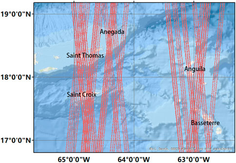
FIGURE 1. Study areas over the Virgin Islands. The red lines in this figure are the ground tracks of ICESat-2 used in the study. The base map data are from World_Ocean_Base produced by ArcGIS 10.1, which is an attribution from Esri, Garmin, GEBCO, NOAA NGDC, and other contributors.

TABLE 1

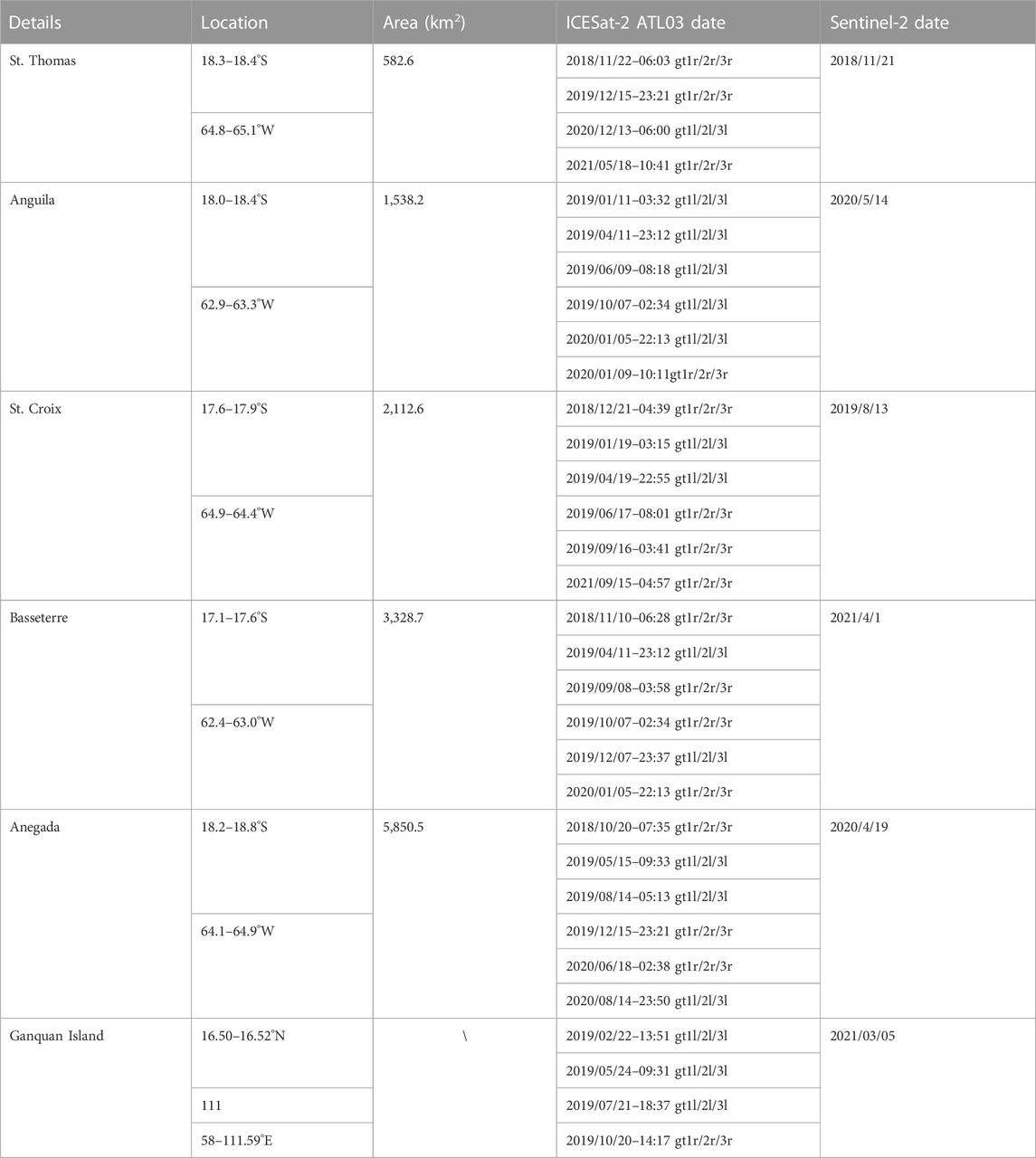
TABLE 1. Detailed information on the study areas and satellite data.

2.2 Satellite data

2.2.1 ICESat-2 data

ICESat-2 ATLAS is a space-based laser altimeter launched in September 2018, which is a photon-counting lidar consisting of three strong-weak beam pairs with a revisit period of 91 days and a distance between laser footprints along the track of only 0.7 m (Altamimi et al., 2016). The distance between each beam pair is 3.3 km, and the spacing on the ground between the strong and weak beams within each pair is 90 m. The laser pairs are divided into a strong beam and a weak beam based on an energy ratio of 1:4, which can effectively improve surface elevation change detection. Each laser has a repetition frequency of 10 kHz at 532 nm wavelength. Each footprint is 70 cm apart and has a diameter of approximately 13 m (Neumann et al., 2013; Neumann et al., 2019). The ICESat-2 geolocation photon data are available in the ATL03 product, which is disseminated through the National Snow and Ice Data Center (NSIDC) (Markus et al., 2017; Neumann et al., 2018). The ATL03 datasets report time, latitude, longitude, and elevation information for each photon above the World Geodetic System (WGS) 84 ellipsoid.

2.2.2 Sentinel-2 imagery

Sentinel-2 data are selected as passive remote sensing imagery for the multispectral features in this study. Sentinel-2, launched in June 2015, is a dual-satellite mission developed by the European Space Agency (ESA) with a revisit period of 5 days (Drusch et al., 2012; NOAA, 2023). Sentinel 2 carries the Multispectral Imager (MSI) that measures remote sensing images for multispectral bathymetry. We used Level-1C (L1C) data, available on the U.S. Geological Survey (USGS) website. The Level-2A (L2A) image data are obtained by atmospheric correction based on L1C data with the Sen2Cor plug-in at SNAP, while the L1C data without atmospheric correction are retained for comparison. Sen2Cor is an L2A processor whose primary purpose is to correct single-date Sentinel-2 L1C top-of-atmosphere products from atmospheric effects to provide L2A bottom-of-atmosphere reflectivity products (Main-Knorn et al., 2017). Band 2 (blue), Band 3 (green), Band 4 (red), Band 5 (vegetation red edge 1, VRE1), Band 6 (vegetation red edge 2, VRE2), Band 7 (vegetation red edge 3, VRE3), Band 8 (near-infrared, NIR) Band 11 (SWIR1) and Band 12 (SWIR2) in Sentinel-2 imagery are applied for our study. The 9 spectral bands chosen in the study cover the range of 490–2,190 nm.

3 Methodology

Figure 2 illustrates a general workflow that is used in this paper. First, Sentinel-2 multispectral images are preprocessed with AC. Additionally, ICESat-2 bathymetric points are extracted from ATLAS ATL03 data as the prior data. Then, the ICESat-2 bathymetric points are aligned with the preprocessed Sentinel-2 images, and the training datasets are extracted from the Sentinel-2 image corresponding to each prior water depth point. Subsequently, the training datasets are input into the machine learning model training. Finally, the other whole bathymetric maps are generated by the trained models. The CUDEM data at St. Thomas are used for validation.

FIGURE 2

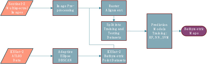
FIGURE 2. Overview of the whole methodology.

3.1 Adaptive ellipse DBSCAN for bathymetric photon detection

When downloading ICESat-2 ATL03 data from the official website, we can narrow the data based on search criteria such as date, longitude and latitude, draw bounding boxes on the Earth’s surface, or import a shape file smaller than 350 points. After obtaining an ATL03 file that passes through the target island, the bathymetric photon points are extracted from ICESat-2 ATL03 data by the following steps. The whole flowchart of the adaptive ellipse DBSCAN algorithm is shown in Figure 3. The input ICESat-2 ATL03 data are intercepted along the vertical elevation direction, and the interception range should roughly include the sea surface and the bottom topography. The ATL03 data are taken as the horizontal axis in the along-track distance direction, and the along-track distance axis is reduced. Then, the data are segmented, and each segment is taken as a photonic signal dataset $\mathrm{D}$. For each segment, the instantaneous sea surface elevation ${\mathrm{S}}_{\mathrm{s}\mathrm{u}\mathrm{f}}$ is calculated, and the photonic data above ${\mathrm{S}}_{\mathrm{d}\mathrm{o}\mathrm{w}\mathrm{n}}$ photon data are removed. Then we compute the Euclidean distance matrix for all points in dataset $\mathrm{D}$ and sort each row element in the distance matrix in ascending order.

FIGURE 3

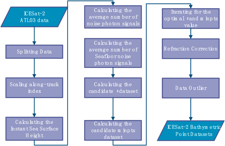
FIGURE 3. Adaptive ellipse DBSCAN algorithm flowchart.

Then the candidate radius $D_{\epsilon }$ is calculated:

$D_{\epsilon }=\left\{{\epsilon }_k=\overline{D_k}\mid 1\le k\le N\right\}(1)$

where $k=\mathrm{1,2},\dots ,N$; $N$ is the length of $D$. $D_k$ is the element of the sorted Euclidean distance matrix of D.

The candidate threshold dataset $D_{mpts}$ is calculated:

$D_{mpts}=\left\{{minpts}_k=\frac{\left(N_{sn}-N_{no}\right)+\ln \left(M\right)}{\ln \left(N_{sn}/N_{no}\right)},1\le k\le N\right\}(2)$

where $N_{sn}$ is the average number of noise photon signals for each ${\epsilon }_k$ and $N_{no}$ is the average number of noise photon signals. $M$ is the number of frames that the original photon divided in the vertical direction. If $D_{mpts}$ is not an integer, then it is rounded up.

Iterate through $k$, and put the corresponding ${\epsilon }_k$ and ${minpts}_k$ into DBSCAN to cluster the photonic signal dataset $D$, and obtain the generated clusters under different k values; when the generated clusters are the same three times in a row, record the cluster as the optimal cluster. Continue clustering until the generated number of clusters is no longer the optimal number of clusters, and choose the maximum $k$ corresponding to when the number of clusters is the optimal number of clusters as the optimal $k$; the radius corresponding to the optimal k and the minimum clustering threshold are the optimal DBSCAN parameters of $D$; put the optimal radius and the minimum clustering threshold into DBSCAN for clustering operation, and obtain the topography corresponding to the current segment data. The preliminary ICESat-2 bathymetric photon points are obtained using the optimal parameters in DBSCAN.

The preliminary ICESat-2 bathymetric photon points then need refraction correction to correct the displacement caused by the refraction of the air/water interface geometry (Parrish et al., 2019). Since the detection results still retain some interference signals, we need to determine outliers or noise that are significantly different or inconsistent with the signal to improve the accuracy. We next apply wavelet filtering to the data, and then, the data are classified into three categories by the K-medoids algorithm. Outlier points along the horizontal and vertical axes were removed. Outliers along the horizontal and vertical axes that differ from the median of the window by more than three scaled median absolute deviations (MADs) are removed.

3.2 Data preprocessing

Before deriving the water depth, Sentinel 2 L1C level images are atmospherically corrected to L2A level products using the SNAP Sen2cor plug-in, followed by a series of preprocessing steps, including subset, cloud and land removal. For comparison, our study examines the results using uncorrected images, which means that the preprocessed L1C images without atmospheric correction are also training datasets. Since the resolution of the ICESat-2 bathymetric points (0.7 m) is different from that of the Sentinel-2 image (10 m), it is necessary to downsample the ICESat-2 bathymetric points at the Sentinel-2 image resolution of 10 m. The ICESat-2 bathymetric point data with high spatial resolution should be matched with the Sentinel-2 images according to their geographical position. Each pixel of the Sentinel-2 image may correspond to multiple ICESat-2 bathymetric point data, so the average of these ICESat-2 bathymetric point data is calculated as the a priori bathymetric data of the pixel. Meanwhile, the Sentinel-2 Rrs vectors of each band corresponding to the ICESat-2 data are taken as the training data. The proportions for training datasets (including validation) and testing were 80% and 20%, respectively.

Furthermore, this research tries several different band combinations, as shown in Table 2, to observe their influence on the prediction models. Band 3 includes the basic natural color bands (red, blue and green). Band 4 adds the NIR band based on natural color. Band 6 adds SWIR1 and SWIR2 compared to band 4. Band 8 covers all selected bands except NIR, while band 9 contains all bands.

TABLE 2

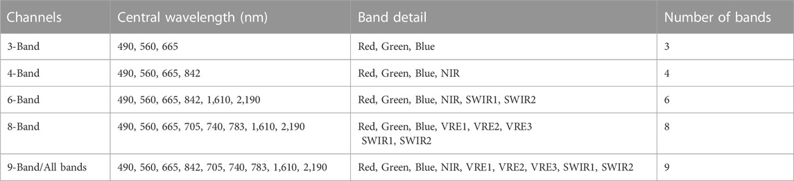
TABLE 2. Sentinel-2 band combinations.

3.3 Prediction model training

Machine learning methods have shown great advantages in regression analysis. In this study, the ICESat-2 bathymetric point datasets extracted in Section 3.2 and the corresponding Sentinel-2 remote sensing reflectances are applied as input vectors for training models. Three typical machine learning predictions are selected to evaluate the capabilities of ICESat-2 bathymetry estimation in this paper, and the linear model (Lyzenga, 1985) and the band ratio model (Stumpf et al., 2003) are also used for comparison. The Random Forest has been noted for its robust generalization ability and capacity to select optimal numbers of features and decision trees for classification or prediction purposes (Manessa et al., 2016). The Neural network models can continually train and optimize their structure’s parameters, thereby producing non-linear water depth inversion results (Lippmann, 1987). The Support Vector Machine approach can effectively fit large volumes of data and identify appropriate approximation functions for bathymetry (Wang et al., 2019). The Sentinel-2 Rrs vectors of the specified band over five study areas were input into the trained model, and the corresponding water depth of that pixel point was obtained. Finally, the retrieved bathymetric map was generated by rearrangement. All prediction models were developed in MATLAB 2022A.

3.3.1 Random forest (RF)

Breiman introduced random forest in 2001 (Breiman, 2001), which is used in recognition, regression, classification and other fields. This model is based on a set of decision trees (forests) that are trained toward the best combination (Kullarni and Sinha, 2013). Random forests are more adapted to data that are high-dimensional and have a large number of samples, so their advantages are also reflected in their excellent performance in dealing with high-dimensional and large quantities of data without artificial data cleaning, feature combination, dealing with sample imbalance, or even vacancy value filling. In this paper, the number of decision trees constructed by the model is considered in random forest. The number of decision trees considered varies from 50 to 200 trees.

3.3.2 Neural network (NN)

A neural network is a parallel computing architecture that can create non-linear multiparameter relationships between reflectances from different spectral bands and water depths (Lippmann, 1987). The processing performed by each neuron in the network includes forming a weighted sum of the inputs, followed by a non-linear transfer function to produce an output (Sandidge and Holyer, 1998). The feedforward network consists of a series of layers. The first layer has a connection from the network input. Each subsequent layer has connections from the previous layer. The final layer produces the output of the network. Feedforward neural networks with enough neurons in the hidden layer can be adapted to any finite input‒output mapping problem. The feedforward neural network used in this study is a two-layer feedforward network with sigmoid hidden neurons and linear output neurons. The number of hidden layer neurons is set to 50. The transfer function is a sigmoid function, and the type of regression is chosen.

3.3.3 Support vector machine (SVM)

SVM is a machine learning method proposed in the 1990s based on statistical learning theory and the principle of structural risk minimization (Vapnik, 1999). SVM is a binary classification model that maps training data into a feature space by means of a kernel function and finds the best hyperplane that separates data points of one class from data points of another class. Different kernel functions can lead to completely different properties (Yang et al., 2021). Popular kernel functions include linear, non-linear, radial basis function (RBF), sigmoid and Gaussian kernel functions, which are suitable for different applications (Agarwal and Kumar, 2016). When there is no prior knowledge about the data, the Gaussian kernel is chosen in this paper with the kernel scale set to $\sqrt{P/4}$, where P is the number of predictors.

3.4 Result assessment

The accuracy of the inverse satellite bathymetry map was verified by comparing the predicted depth with the in situ depth in St. Thomas. In other regions, the results were evaluated by comparing predicted depths with ICESat-2 bathymetric point data. Metrics such as root mean squared error (RMSE), coefficient of determination (R²), MAE (mean absolute error), and bias are used to evaluate the effectiveness of the regression models.

$RMSE=\sqrt{{\sum }_{i=1}^N{\left(d_{reali}-d_{prediti}\right)}^2/N}(3)$

$R^2=1-\frac{{\sum }_{i=1}^N{\left(d_{reali}-d_{prediti}\right)}^2}{{\sum }_{i=1}^N{\left(d_{reali}-\overline{d_{predit}}\right)}^2}(4)$

$MAE={\sum }_{i=1}^N\left|d_{reali}-d_{prediti}\right|/N(5)$

$Bias={\sum }_{i=1}^N\left(d_{reali}-d_{prediti}\right)/N(6)$

where $d_{real}$ is the measured depth, $d_{predit}$ is the predicted depth corresponding to $d_{real}$, $\overline{d_{predit}}$ is the mean value of the predicted depth and $N$ is the length of the dataset.

4 Results

4.1 Bathymetric photon detection using AE-DBSCAN

Figure 4A shows the Sentinel-2 basemap on 21 November 2018. The red line indicates the laser track of ICESat-2 on 18 May 2021, and the yellow line on the red line indicates the location of the sounding results shown in this section. The purple lines named Site A and Site B indicate the positions of bathymetric profiles in Section 5.1. To evaluate the SDB results using separate training in each region, Sites A and B in Figure Figure4A are selected to present bathymetric inversion results. Sites A and B are located in the same coastal waters of St. Thomas, but have different water conditions and different images. Figures 4B,C show the results of ICESat-2 seafloor signal detection using AE-DBSCAN and the standard DBSCAN with fixed $\mathrm{\epsilon }$ =1.0 m and $Minpts$ =5. Figures 4D,E show the corresponding scatter plots of ICESat-2 bathymetric point depth vs. in situ depth.

FIGURE 4

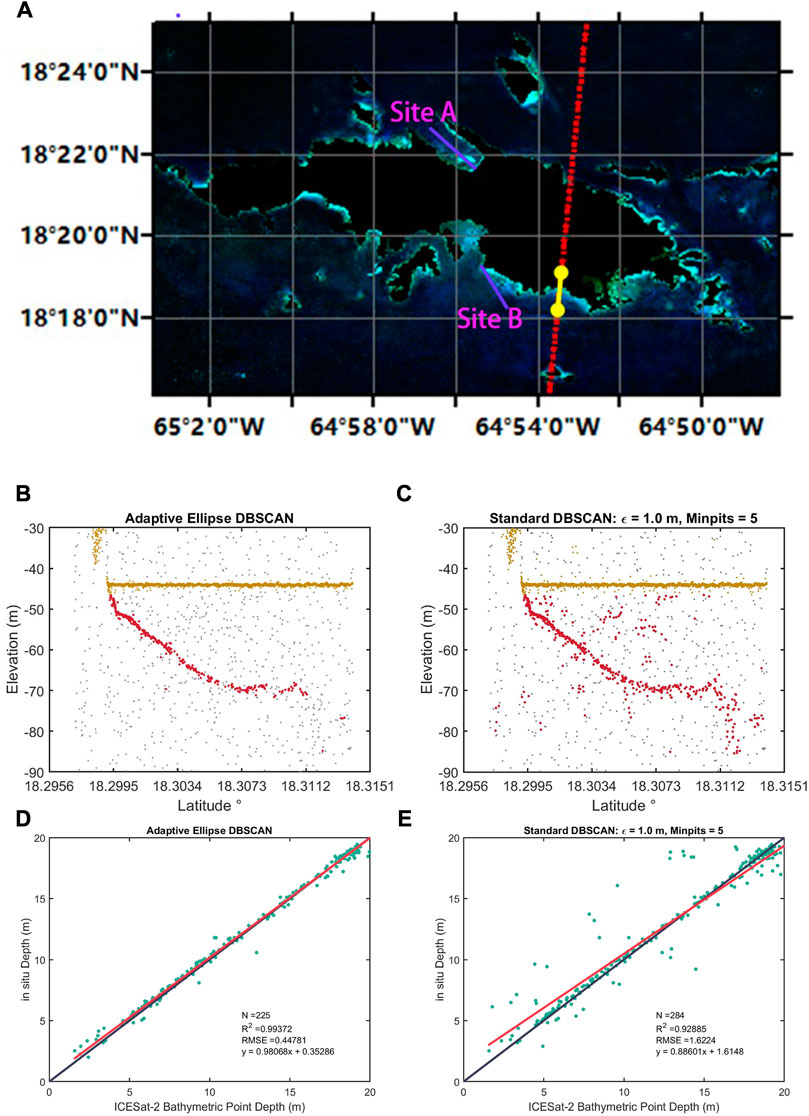
FIGURE 4. (A) The Sentinel-2 basemap in St. Thomas: the red line presents the laser trajectories of ICESat-2 on 18 May 2021, and the yellow line on the red trajectory indicates the detection result position shown in this section. The RGB background satellite imagery was obtained by Sentinel-2 on 21 November 2018. The detection comparison using different DBSCAN algorithms. The original detected seafloor photons red, the detected sea surface is yellow, and the original photons are grey: (B) AE-DBSCAN; (C) standard DBSCAN with fixed $\mathrm{\epsilon }=1.0\mathrm{m}$; $Minpts=5$. The corresponding error scatter plots of ICESat-2 bathymetric point depth vs. in situ depth: (D) AE-DBSCAN; (E) standard DBSCAN with fixed $\mathrm{\epsilon }=1.0\mathrm{m}$ and $Minpts=5$.

Figures 4B,C illustrate that the results using the AE-DBSCAN algorithm can better track the ICESat-2 seafloor return signal photons since the adaptive $\mathrm{\epsilon }$ and $Minpts$ adapt to the variation in photon signal density. In contrast, the standard DBSCAN retains many unnecessary noise points due to the fixed threshold, which affects the subsequent results. As illustrated in Figure 4D, the AE-DBSCAN tends to fit the in situ data. The AE-DBSCAN result yields an overall accuracy of 0.44 m with an R² of 0.99. For comparison, the standard DBSCAN yields a lower accuracy of approximately 1.62 m with an R² of 0.92.

4.2 Validation

Figure 5A demonstrates the in situ bathymetric map in St. Thomas and Figures 5B–F demonstrate the bathymetric maps there using the random forest model with different band combinations. All bathymetric results are generated consistently for all depth ranges up to 20 m, beyond the slope into the open ocean shown as dark blue in maps. The SDB results using the random forest (RF) algorithm with different band combinations exhibit qualitatively good agreement with those identifiable in the in situ data. All SDB results efficiently describe the nearshore depth with good precision. Overall, SDB maps retrieved the depth gradient with high accuracy as in the CUDEM map from coastal zones to the open ocean.

FIGURE 5

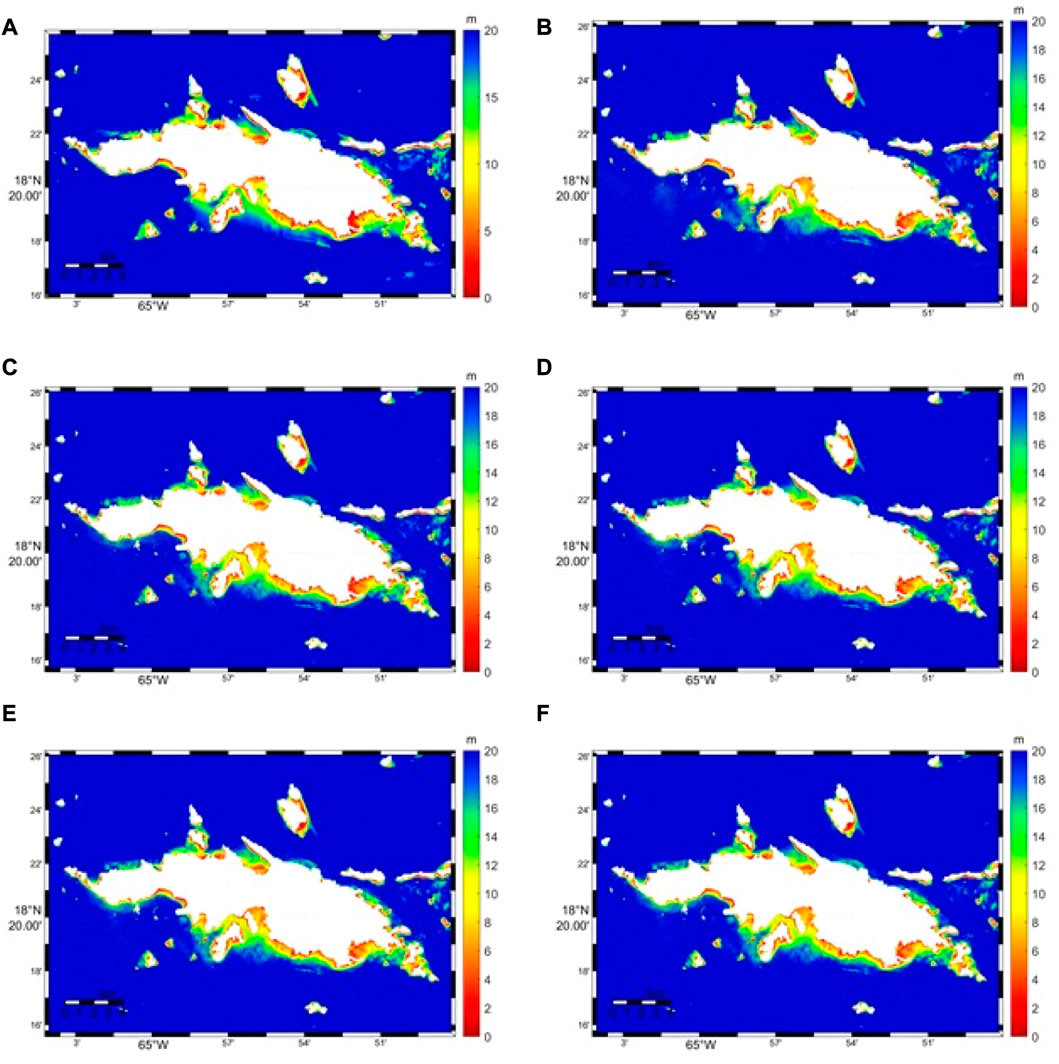
FIGURE 5. The bathymetric maps in St. Thomas: (A) CUDEM depth; (B) SDB map using random forest with 3-Band; (C) SDB map using random forest with 4-Band; (D) SDB map using random forest with 6-Band; (E) SDB map using random forest with 8-Band; (F) SDB map using random forest model with 9-Band.

Figures 6A–F show the validation of the random forest-estimated depth with different band combinations vs. in situ depth in St. Thomas. For the retrieved depths in St. Thomas, the results using RF with 8-Band and 9-Band have comparable best performances with respective ranges of RMSE of 1.35 m and R² of 0.97, with slightly lower errors found in the result using RF with 8-Band. The worst result is obtained by using RF with 3-Band with an RMSE value of 1.45 m and an R² of 0.96. These other calibration results produce RMSEs of 1.36 m and 1.31 m and R² values of 0.97 and 0.97 when using RF with 4-Band and 6-Band, respectively. The majority of the points follow the 1:1 line, as shown in these scatter plots, indicating good performance using RF with different band combinations, and all RMSEs are less than 8% of the maximum depth. The ICESat-2 bathymetry data are used to evaluate the bathymetry results. Figure 6F shows the scatter plot of the random forest-estimated depth with the 3-Band vs. ICESat-2 bathymetric point depth with an RMSE of 1.51 m and an R² of approximately 0.97.

FIGURE 6

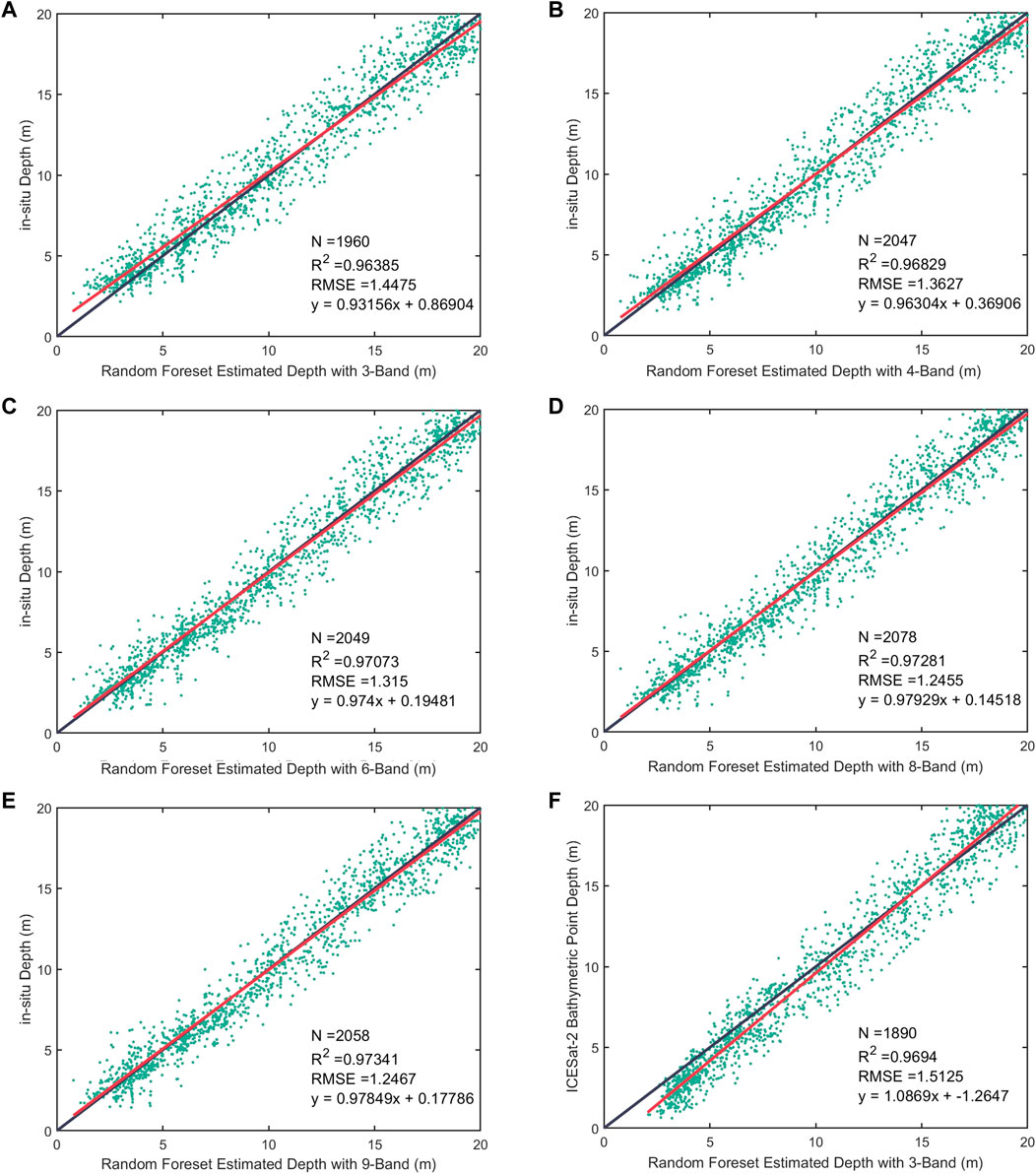
FIGURE 6. The error scatter plots of random forest-estimated depth vs. in situ depth in St. Thomas using different band combinations: (A) 3-Band; (B) 4-Band; (C) 6-Band; (D) 8-Band; (E) 9-Band; (F) scatter plot of random forest-estimated depth vs. ICESat-2 bathymetric point depth.

4.3 Bathymetric retrieval maps

Figures 7A,C,E,G show SDB maps in Anguila, Basseterre, St. Croix and Anegada using random forest with 3-Band, respectively. Figures 7B,D,F,H show the scatter plots of the random forest-estimated depth with 3-Band vs. ICESat-2 bathymetric point depth corresponding to the left map. The SDB maps at the four sites depict the shallow water area within 0–20 m. In these study areas, since no in situ bathymetric data are available, the ICESat-2 bathymetric data are used to evaluate the bathymetric results derived from the ICESat-2 bathymetric points and Sentinel-2 images alternatively. The scatter result using random forest (RF) with 3-Band in St. Thomas has the best R² with a value of approximately 0.97 (Figure 6F), while the other SDB error scatter plots in Anguila, Basseterre, St. Croix and Anegada have comparable performances with respective ranges of an R² of approximately 0.96. The RMSE values within the same depth range in St. Thomas, Anguila, Basseterre, St. Croix and Anegada are 1.51 m, 1.77 m, 1.69 m, 1.46 m and 1.44 m, respectively, which are all less than 10% of the maximum depths. Table 3 lists the accuracy assessment parameters for all the selected islands using RF with 4-Band and 9-Band. The bathymetric map in St. Croix produces a less significant error compared to other locations with a higher R² and lower RMSE. Overall, the table indicates that the accuracy tends to increase with the number of training bands.

FIGURE 7

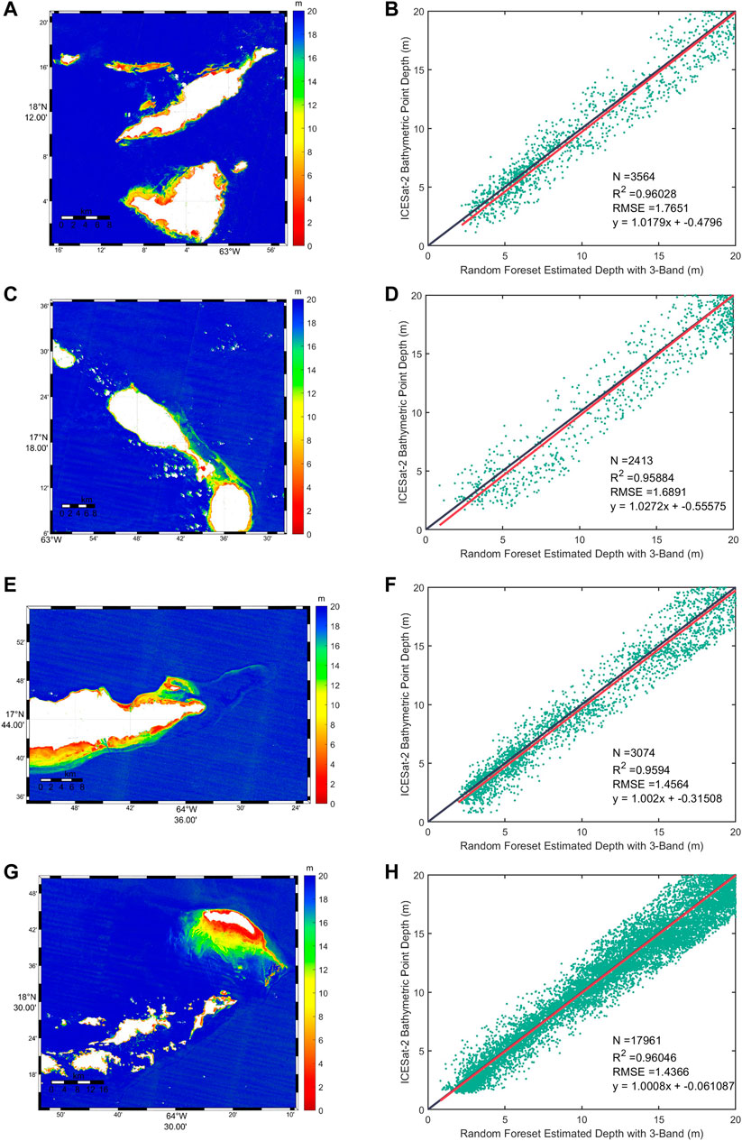
FIGURE 7. SDB map at different sites using random forest with 3-Band: (A) Anguila; (C) Basseterre; (E) St. Croix; (G) Anegada. The error scatter plots of Random forest-estimated depth with 3-Band vs. ICESat-2 bathymetric point depth over different sites: (B) Anguila; (D) Basseterre; (F) St. Croix; (H) Anegada.

TABLE 3

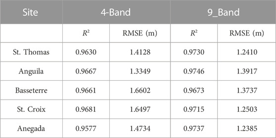
TABLE 3. Accuracy assessment of random forest-estimated depth vs. ICESat-2 bathymetric point depth for all the islands with 4-Band and 9_Band.

5 Discussion

5.1 Validation over different area

In order to demonstrate the efficacy of machine learning techniques in predicting bathymetry in different waters, we conducted the active and passive satellite data presented in Table 1 at Ganquan Island. Using the RF, NN, and SVM models with 3-Band, we generate SDB maps at Ganquan Island, as depicted in Figures 8A–C. The results obtained from each model demonstrated a similar trend in bathymetric estimation from shallow to deep waters. To validate our findings, we utilized in situ data collected by the Shanghai Institute of Optics and Fine Mechanics (SIOM), Chinese Academy of Sciences (CAS), via an airborne LiDAR instrument (Chen et al., 2021a; Liu et al., 2021). Table 4 lists the accuracy assessment of estimated depths compared to the in situ depths at Ganquan Island, employing diffirent prediction models. Notably, RF yielded the highest R² value (0.965), followed by SVM (0.952), while NN has the lowest R² (0.949). The ranking order remains consistent for the RMSE and MAE fit results as well. Overall, the results indicate that machine learning could produce stable and reliable inversion results for bathymetry at Ganquan Island in the South China Sea.

FIGURE 8

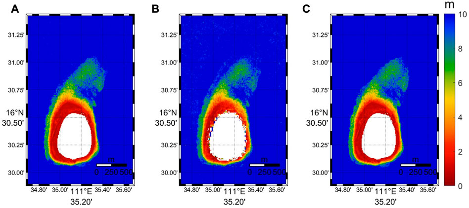
FIGURE 8. SDB map at Ganquan Island using different models with 3-Band: (A) RF; (B)NN; (C)SVM.

TABLE 4

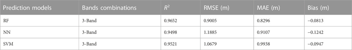
TABLE 4. Accuracy assessment of estimated depth vs. in situ depth using different prediction models at Ganquan Island.

5.2 Comparison of different SDB models

Table 5 presents the summary accuracy assessment in St. Thomas with R², RMSE, MAE and bias for three machine learning prediction models and two empirical models with 3-Band and 9-Band. The R² values within 3-Band for RF, NN, SVM and the linear model are 0.96, 0.94, 0.96 and 0.82, and the corresponding RMSEs are 1.44 m, 1.69 m, 1.48 m and 2.19 m, respectively. Among them, the RF model fits the in situ data best, while the empirical linear model provides the worst results. The fitting results of the band ratio model are followed by the results of the NN and are better than those of the linear model. Note that all the bias values are positive, which means that the SDB results predict shallower depths than the in situ depths. Similarly, the results with 9-Band are better than those with 3-Band, where the best result is obtained using RF. Overall, the ML-based SDB achieved an overall RMSE of less than 1.5 m in St. Thomas better than traditional empirical models, which shows the advantage of ml models in establishing non-linear relationships between Rrs and depth.

TABLE 5

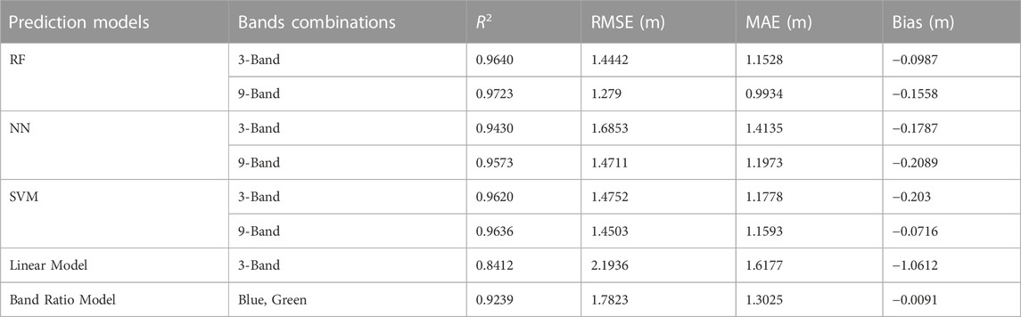
TABLE 5. Accuracy assessment of estimated depth vs. in situ depth using different prediction models in St. Thomas.

More detailed cross-sections at Site A and Site B are provided in Figure 9. The first cross profile (Figure 9A) compares different estimated depths using different prediction models and in situ depths from the south around the nearshore area to the north estuary. The errors generated by the SVM and NN models occur at almost all depth levels, especially in very shallow areas. Figure 9B shows a similar trend. The difference between the predicted depths using the RF model and the in situ depths is stable within 6 m, so the RF model produces a good fit with the in situ data compared with other models in St. Thomas. Comparatively, the RF model has a high degree of flexibility and can be used to create suitable models if a large quantity of training data is available.

FIGURE 9

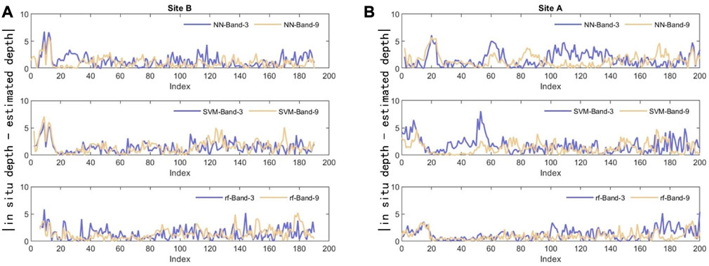
FIGURE 9. Bathymetric cross profiles at Sites A and B over St. Thomas showing a comparison between the RF model and in situ depths: (A) Site A; (B) Site B.

5.3 Comparison of different band combinations

To verify the chosen band combinations in the RF model, Figure 10A shows the RMSE graph for the increment of 1 m depth, which illustrates that all band combinations improve the accuracy with increasing depth. In the shallow water region within 8 m, the results of each band combination do not differ significantly. 4-Band achieves higher accuracy than 6-Band except in the 5–7 m depth range. In general, the RMSE of the result using 8-Band is overall lowest among the combinations in St. Thomas except at the 4 m depth range, and the accuracy using 9-Band is very close to that of 8-Band, followed by the results using 6-Band, and 3-Band gives the worst result. As shown in Figures 6D,E, the scatter plot in St. Thomas using RF with 8-Band and 9-Band also provides similar excellent performance. This is because the number of bands affects the decision result of adjusting the decision tree in the random forest. The more bands involved in training, the richer the decision results obtained, and it will determine the accuracy (Belgiu and Drăguţ, 2016). However, increasing the number of bands infinitely upward causes overfitting and makes the performance worse, and setting a reasonable number of training bands is also important for prediction accuracy.

FIGURE 10

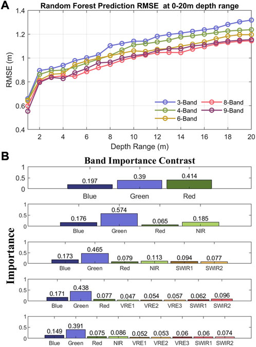
FIGURE 10. (A) Random forest prediction RMSE graph for each increment of 1 m in depth; (B) predictor importance estimates in random forest training.

Figure 10B illustrates the importance of the bands in the RF model. Regardless of the band combination, the green band contributes the most to the tree nodes and has the highest feature importance, which greatly affects the RF model construction and accuracy, followed by the blue band except 3-Band. Due to the high transparency of the blue and green bands in water, the light from the two bands can penetrate deeper water, and their reflectance is very important for the bathymetric inversion results (He et al., 2021). In the three combinations containing the NIR band (i.e., 4-Band, 6-Band and 9-Band), the importance of the NIR band is higher than that of the red band, which indicates that the NIR band has the potential to replace the role of the RED band in training. However, the importance difference between the two bands decreases as the number of bands increases, indicating that the addition of other bands dilutes the importance of red and NIR bands. The VRE and SWIR bands are easily absorbed in the water and are less important in model training.

5.4 Comparison of SDB with and without atmospheric correction

The Rrs information received by the MSI includes the reflection from the water surface, the water body and the water bottom and atmospheric reflection. The Sen2Cor atmospheric correction procedure eliminates the influence of atmospheric contribution (Toming et al., 2016). Figure 11A depicts the RMSE values using Sentinel-2 images without atmospheric correction for each increment of 1 m, indicating that the accuracy tends to increase as the depth range increases. When the water depth range is greater than 10 m, the RMSE of the results using 4-Band is the smallest with the highest accuracy, followed by the results using 6-Band, 8-Band and 9-Band, and the results of 3-Band are still the worst. Compared to Figure 10A, the overall values of RMSE using Sentinel-2 images without AC are larger for bathymetry inversion, indicating that atmospheric correction helps to improve the accuracy of bathymetric inversion.

FIGURE 11

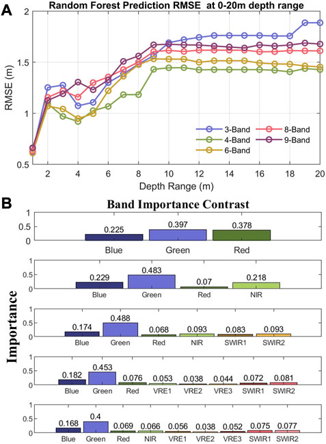
FIGURE 11. (A) Random forest prediction RMSE graph using Sentinel-2 images without atmospheric correction for each increment of 1 m depth; (B) predictor importance estimates in random forest training using Sentinel-2 images without atmospheric correction.

Figure 11B illustrates the predictor importance estimates in random forest training using Sentinel-2 images without atmospheric correction. Similar to the results shown in Figure 10B, the blue and green bands are still very important in RF model training using Sentinel-2 images without AC. Since the images are not atmospherically corrected, the importance of the red band is increased, surpassing the blue band in 3-Band and the NIR band in 9-Band. When using the NIR band, lands, clouds and Sun glint signals can be masked (Mishra et al., 2005; Lyzenga et al., 2006). Thus, the NIR band is a very important band in atmospheric correction (Wang et al., 2012), and atmospheric correction based on the NIR band is also widely used (Gordon and Wang, 1994; Wang, 2016). When training the model using the Rrs vectors without atmospheric correction, including the NIR band helps to improve the training accuracy. Machine learning makes use of the NIR band for atmospheric correction, thus eliminating the need for atmospheric correction. However, when the number of bands reaches saturation, other bands share the role of the NIR bands, making the accuracy of the results using 9-Band lower than those of 8-Band.

ICESat-2 bathymetry data are used to evaluate the accuracy of bathymetry inversion using Sentinel-2 images without atmospheric correction for the five islands. Table 6 summarizes the accuracy assessment parameters using the RF model with 4-Band and 9-Band. The inversion accuracy of Anegada is relatively good, with an R² of 0.97 and an RMSE of 1.24 m among the results using 4-Band and St. Croix is consistent with an R² of 0.97 and an RMSE of 1.40 m for the results using 4-Band. This indicates the potential application of depth inversion using remote sensing images without atmospheric correction, which helps to improve efficiency.

TABLE 6

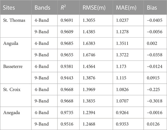
TABLE 6. Accuracy assessment of random forest-estimated depth using Sentinel-2 images without atmospheric correction vs. ICESat-2 bathymetric point depth for all the islands with 4-Band and 9-Band.

6 Conclusion

In this study, we proposed an active and passive remote sensing combined SDB method using only satellite data. We employed three machine learning methods and the performances compared with conventional empirical SDB models are presented. The results show that compared to the standard DBSCAN method, the AE-DBSCAN method we used in seafloor return signal detection can achieve higher accuracy with an RMSE of 0.44 m and an R² of 0.99, benefiting from an adaptive process and changeable key parameters that can adapt well to photon density variations. Additionally, the a priori bathymetric point data derived from ICESat-2 are consistent with the in situ data in St. Thomas, and the bathymetric inversion results using random forest for bathymetric inversion combined with Sentinel-2 images also maintain high accuracy with the in situ data in St. Thomas, with an RMSE of less than 1.5 m.

Furthermore, the ML-based SDB achieved an overall RMSE of less than 1.5 m in St. Thomas better than the traditional empirical SDB method, and the accuracy of bathymetric inversion using the random forest model outperformed the neural network and SVM models. Using the random forest model, the higher the number of bands, the higher the inversion accuracy, but 8-Band is optimal and slightly higher than the accuracy of 9-Band. The inversion results using Sentinel-2 images without AC with RMSEs less than 2 m are inferior to those using Sentinel-2 images with AC, but it is still an attempt to help improve the efficiency of bathymetric inversion by avoiding a complex atmospheric correction process. In the future, the present method will help build global nearshore bathymetric datasets using only satellite data in large-scale regions, and the retrieval of global SDBs will greatly benefit from the large datasets constructed in this paper. (Coastal and Marine Ecosystem, 2022).

Data availability statement

The original contributions presented in the study are included in the article/Supplementary Material, further inquiries can be directed to the corresponding author.

Author contributions

ZZ performed the preprocessing of the remote sensing data. CX conceived, wrote and designed the manuscript, and PC and DP supervised, wrote-reviewed, and edited the manuscript.

Funding

This research was funded by the National Key Research and Development Program of China (2022YFB3901703), the Key Special Project for Introduced Talents Team of Southern Marine Science and Engineering Guangdong Laboratory (GML2019ZD0602), the National Natural Science Foundation (42276180; 41901305; 61991453), and the Key Research and Development Program of Zhejiang Province (2020C03100).

Acknowledgments

We thank the reviewers for their suggestions, which significantly improved the presentation of the paper.

Conflict of interest

The authors declare that the research was conducted in the absence of any commercial or financial relationships that could be construed as a potential conflict of interest.

Publisher’s note

All claims expressed in this article are solely those of the authors and do not necessarily represent those of their affiliated organizations, or those of the publisher, the editors and the reviewers. Any product that may be evaluated in this article, or claim that may be made by its manufacturer, is not guaranteed or endorsed by the publisher.

References

Agarwal, D. K., and Kumar, R. (2016). Spam filtering using SVM with different kernel functions. Int. J. Comput. Appl. 136, 16–23. doi:10.5120/ijca2016908395

CrossRef Full Text | Google Scholar

Albright, A., and Glennie, C. (2021). Nearshore bathymetry from fusion of sentinel-2 and ICESat-2 observations. IEEE Geoscience Remote Sens. Lett. 18, 900–904. doi:10.1109/lgrs.2020.2987778

CrossRef Full Text | Google Scholar

Altamimi, Z., Rebischung, P., MéTIVIER, L., and Collilieux, X. (2016). ITRF2014: A new release of the international terrestrial reference frame modeling nonlinear station motions. J. Geophys. Res. Solid Earth 121, 6109–6131. doi:10.1002/2016jb013098

CrossRef Full Text | Google Scholar

Auret, L., and Aldrich, C. (2012). Interpretation of nonlinear relationships between process variables by use of random forests. Miner. Eng. 35, 27–42. doi:10.1016/j.mineng.2012.05.008

CrossRef Full Text | Google Scholar

Belgiu, M., and Drăguţ, L. (2016). Random forest in remote sensing: A review of applications and future directions. ISPRS J. Photogrammetry Remote Sens. 114, 24–31. doi:10.1016/j.isprsjprs.2016.01.011

CrossRef Full Text | Google Scholar

Botha, E. J., Brando, V. E., and Dekker, A. G. (2016). Effects of per-pixel variability on uncertainties in bathymetric retrievals from high-resolution satellite images. Remote Sens. 8, 459. doi:10.3390/rs8060459

CrossRef Full Text | Google Scholar

Bramante, J. F., Raju, D. K., and Sin, T. M. (2013). Multispectral derivation of bathymetry in Singapore's shallow, turbid waters. Int. J. Remote Sens. 34, 2070–2088. doi:10.1080/01431161.2012.734934

CrossRef Full Text | Google Scholar

Breiman, L. (2001). Random forests. Mach. Learn. 45, 5–32. doi:10.1023/a:1010933404324

CrossRef Full Text | Google Scholar

Chen, P., Jamet, C., Zhang, Z., He, Y., Mao, Z., Pan, D., et al. (2021a). Vertical distribution of subsurface phytoplankton layer in South China Sea using airborne lidar. Remote Sens. Environ. 263, 112567. doi:10.1016/j.rse.2021.112567

CrossRef Full Text | Google Scholar

Chen, Y., Le, Y., Zhang, D., Wang, Y., Qiu, Z., and Wang, L. (2021b). A photon-counting LiDAR bathymetric method based on adaptive variable ellipse filtering. Remote Sens. Environ. 256, 112326. doi:10.1016/j.rse.2021.112326

CrossRef Full Text | Google Scholar

ChéNIER, R., Faucher, M.-A., and Ahola, R. (2018). Satellite-derived bathymetry for improving Canadian hydrographic service charts. ISPRS Int. J. Geo-Information 7, 306. doi:10.3390/ijgi7080306

CrossRef Full Text | Google Scholar

Coastal and Marine Ecosystems, (2022). Coastal and marine ecosystems-marine jurisdictions. https://web.archive.org/web/20120419075053/http://earthtrends.wri.org/text/coastal-marine/variable-61.html.

Google Scholar

Drusch, M., Del Bello, U., Carlier, S., Colin, O., Fernandez, V., Gascon, F., et al. (2012). Sentinel-2: ESA's optical high-resolution mission for GMES operational services. Remote Sens. Environ. 120, 25–36. doi:10.1016/j.rse.2011.11.026

CrossRef Full Text | Google Scholar

Ester, M., Kriegel, H.-P., Sander, J., and Xu, X. (1996). “A density-based algorithm for discovering clusters in large spatial databases with noise,” in Proceedings of the Second International Conference on Knowledge Discovery and Data Mining, Portland, Oregon, Auguest 1996.

Google Scholar

Forfinski-Sarkozi, N. A., and Parrish, C. E. (2016). Analysis of MABEL bathymetry in keweenaw bay and implications for ICESat-2 ATLAS. Remote Sens. 8, 772. doi:10.3390/rs8090772

CrossRef Full Text | Google Scholar

Gao, J. (2009). Bathymetric mapping by means of remote sensing: Methods, accuracy and limitations. Prog. Phys. Geogr. Earth Environ. 33, 103–116. doi:10.1177/0309133309105657

CrossRef Full Text | Google Scholar

Goodman, J. A., Lee, Z., and Ustin, S. L. (2008). Influence of atmospheric and sea-surface corrections on retrieval of bottom depth and reflectance using a semi-analytical model: A case study in kaneohe bay, Hawaii. Appl. Opt. 47, F1–F11. doi:10.1364/ao.47.0000f1

PubMed Abstract | CrossRef Full Text | Google Scholar

Gordon, H. R., and Wang, M. (1994). Retrieval of water-leaving radiance and aerosol optical thickness over the oceans with SeaWiFS: A preliminary algorithm. Appl. Opt. 33, 443–452. doi:10.1364/ao.33.000443

PubMed Abstract | CrossRef Full Text | Google Scholar

He, J., Lin, J., Ma, M., and Liao, X. (2021). Mapping topo-bathymetry of transparent tufa lakes using UAV-based photogrammetry and RGB imagery. Geomorphology 389, 107832. doi:10.1016/j.geomorph.2021.107832

CrossRef Full Text | Google Scholar

Ilori, C. O., and Knudby, A. (2020). An approach to minimize atmospheric correction error and improve physics-based satellite-derived bathymetry in a coastal environment. Remote Sens. 12, 2752. doi:10.3390/rs12172752

CrossRef Full Text | Google Scholar

Jasinski, M. F., Stoll, J. D., Cook, W. B., Ondrusek, M., Stengel, E., and Brunt, K. (2016). Inland and near-shore water profiles derived from the high-altitude multiple altimeter beam experimental lidar (MABEL). J. Coast. Res. 76, 44–55. doi:10.2112/si76-005

PubMed Abstract | CrossRef Full Text | Google Scholar

Kaloop, M. R., El-Diasty, M., Hu, J. W., and Zarzoura, F. (2022). Hybrid artificial neural networks for modeling shallow-water bathymetry via satellite imagery. IEEE Trans. Geoscience Remote Sens. 60, 1–11. doi:10.1109/tgrs.2021.3107839

CrossRef Full Text | Google Scholar

Kullarni, V., and Sinha, P. (2013). Random forest classifier: A survey and future research directions. Int. J. Adv. Comput. 36, 1144–1156.

Google Scholar

Lippmann, R. (1987). An introduction to computing with neural nets. IEEE ASSP Mag. 4, 4–22. doi:10.1109/massp.1987.1165576

CrossRef Full Text | Google Scholar

Liu, C., Qi, J., Li, J., Tang, Q., Xu, W., Zhou, X., et al. (2021). Accurate refraction correction—assisted bathymetric inversion using ICESat-2 and multispectral data. Remote Sens. 13, 4355. doi:10.3390/rs13214355

CrossRef Full Text | Google Scholar

Lyzenga, D. R. (1978). Passive remote sensing techniques for mapping water depth and bottom features. Appl. Opt. 17, 379–383. doi:10.1364/ao.17.000379

PubMed Abstract | CrossRef Full Text | Google Scholar

Lyzenga, D. R., Malinas, N. P., and Tanis, F. J. (2006). Multispectral bathymetry using a simple physically based algorithm. IEEE Trans. Geoscience Remote Sens. 44, 2251–2259. doi:10.1109/tgrs.2006.872909

CrossRef Full Text | Google Scholar

Lyzenga, D. R. (1985). Shallow-water bathymetry using combined lidar and passive multispectral scanner data. Int. J. Remote Sens. 6, 115–125. doi:10.1080/01431168508948428

CrossRef Full Text | Google Scholar

Ma, Y., Xu, N., Liu, Z., Yang, B., Yang, F., Wang, X. H., et al. (2020). Satellite-derived bathymetry using the ICESat-2 lidar and Sentinel-2 imagery datasets. Remote Sens. Environ. 250, 112047. doi:10.1016/j.rse.2020.112047

CrossRef Full Text | Google Scholar

Main-Knorn, M., Pflug, B., Louis, J., Debaecker, V., MüLLER-Wilm, U., and Gascon, F. (2017). Sen2Cor for sentinel-2. Image Signal Process. Remote Sens. XXIII 10427. doi:10.1117/12.2278218

CrossRef Full Text | Google Scholar

Manessa, M., Kanno, A., Sekine, M., Haidar, M., Yamamoto, K., Imai, T., et al. (2016). SATELLITE-DERIVED bathymetry using random forest algorithm and WORLDVIEW-2 imagery. Geoplanning J. Geomatics Plan. 3, 117. doi:10.14710/geoplanning.3.2.117-126

CrossRef Full Text | Google Scholar

Markus, T., Neumann, T., Martino, A., Abdalati, W., Brunt, K., Csatho, B., et al. (2017). The Ice, cloud, and land elevation satellite-2 (ICESat-2): Science requirements, concept, and implementation. Remote Sens. Environ. 190, 260–273. doi:10.1016/j.rse.2016.12.029

CrossRef Full Text | Google Scholar

Mateo-PéREZ, V., Corral-Bobadilla, M., Ortega-FernáNDEZ, F., and RodríGUEZ-MontequíN, V. (2021). Determination of water depth in ports using satellite data based on machine learning algorithms. Energies 14, 2486. doi:10.3390/en14092486

CrossRef Full Text | Google Scholar

Mishra, D. R., Narumalani, S., Rundquist, D., and Lawson, M. (2005). High-resolution ocean color remote sensing of benthic habitats: A case study at the roatan island, Honduras. IEEE Trans. Geoscience Remote Sens. 43, 1592–1604. doi:10.1109/tgrs.2005.847790

CrossRef Full Text | Google Scholar

Misra, A., Vojinovic, Z., Ramakrishnan, B., Luijendijk, A., and Ranasinghe, R. (2018). Shallow water bathymetry mapping using Support Vector Machine (SVM) technique and multispectral imagery. Int. J. Remote Sens. 39, 4431–4450. doi:10.1080/01431161.2017.1421796

CrossRef Full Text | Google Scholar

National Oceanic and Atmospherc Administration, (2023). NOAA continuously updated digital elevation model (CUDEM) - ninth arc-second resolution bathymetric-topographic tiles. https://coast.noaa.gov/htdata/raster2/elevation/NCEI_ninth_Topobathy_2014_8483/.

Google Scholar

Neumann, T. A., Martino, A. J., Markus, T., Bae, S., Bock, M. R., Brenner, A. C., et al. (2019). The Ice, cloud, and land elevation satellite – 2 mission: A global geolocated photon product derived from the advanced topographic laser altimeter system. Remote Sens. Environ. 233, 111325. doi:10.1016/j.rse.2019.111325

CrossRef Full Text | Google Scholar

Neumann, T., Brenner, A., Hancock, D., Robbins, J., Saba, J., Harbeck, K., et al. (2018). Algorithm theoretical basis document (ATBD) for global geolocated photons ATL03. Greenbelt, Maryland: Goddard Space Flight Center.

Google Scholar

Neumann, T., Scott, V. S., Markus, T., and Mcgill, M. (2013). The multiple altimeter beam experimental lidar (MABEL): An airborne simulator for the ICESat-2 mission. J. Atmos. Ocean. Technol. 30, 345–352. doi:10.1175/jtech-d-12-00076.1

CrossRef Full Text | Google Scholar

Parker, H., and Sinclair, M. (2012). The successful application of Airborne LiDAR Bathymetry surveys using latest technology. Oceans - Yeosu 21-24, 1–4.

CrossRef Full Text | Google Scholar

Parrish, C. E., Magruder, L. A., Neuenschwander, A. L., Forfinski-Sarkozi, N., Alonzo, M., and Jasinski, M. (2019). Validation of ICESat-2 ATLAS bathymetry and analysis of ATLAS’s bathymetric mapping performance. Remote Sens. 11, 1634. doi:10.3390/rs11141634

CrossRef Full Text | Google Scholar

Sandidge, J. C., and Holyer, R. J. (1998). Coastal bathymetry from hyperspectral observations of water radiance. Remote Sens. Environ. 65, 341–352. doi:10.1016/s0034-4257(98)00043-1

CrossRef Full Text | Google Scholar

Stumpf, R. P., Holderied, K., and Sinclair, M. (2003). Determination of water depth with high-resolution satellite imagery over variable bottom types. Limnol. Oceanogr. 48, 547–556. doi:10.4319/lo.2003.48.1_part_2.0547

CrossRef Full Text | Google Scholar

Toming, K., Kutser, T., Laas, A., Sepp, M., Paavel, B., and NõGES, T. (2016). First experiences in mapping lake water quality parameters with sentinel-2 MSI imagery. Remote Sens. 8, 640. doi:10.3390/rs8080640

CrossRef Full Text | Google Scholar

Tonion, F., Pirotti, F., Faina, G., and Paltrinieri, D. (2020). A machine learning approach to multispectral satellite derived bathymetry. ISPRS Ann. Photogramm. Remote Sens. Spat. Inf. Sci. V- 3-2020, 565–570. doi:10.5194/isprs-annals-v-3-2020-565-2020

CrossRef Full Text | Google Scholar

Vapnik, V. N. (1999). An overview of statistical learning theory. IEEE Trans. neural Netw. 10, 988–999. doi:10.1109/72.788640

PubMed Abstract | CrossRef Full Text | Google Scholar

Wang, L., Liu, H., Su, H., and Wang, J. (2019). Bathymetry retrieval from optical images with spatially distributed support vector machines. GIScience Remote Sens. 56, 323–337. doi:10.1080/15481603.2018.1538620

CrossRef Full Text | Google Scholar

Wang, M. (2010). Atmospheric Correction for remotely-sensed ocean-colour products. Nova Scotia, Canada: International Ocean-Colour Coordinating Group.

Google Scholar

Wang, M. (2016). Rayleigh radiance computations for satellite remote sensing: Accounting for the effect of sensor spectral response function. Opt. Express 24, 12414–12429. doi:10.1364/oe.24.012414

PubMed Abstract | CrossRef Full Text | Google Scholar

Wang, M., Shi, W., and Jiang, L. (2012). Atmospheric correction using near-infrared bands for satellite ocean color data processing in the turbid Western Pacific region. Opt. Express 20, 741–753. doi:10.1364/oe.20.000741

PubMed Abstract | CrossRef Full Text | Google Scholar

Wang, Y., Zhou, X., Li, C., Chen, Y., and Yang, L. (2020). Bathymetry model based on spectral and spatial multifeatures of remote sensing image. IEEE Geoscience Remote Sens. Lett. 17, 37–41. doi:10.1109/lgrs.2019.2915122

CrossRef Full Text | Google Scholar

WöLFL, A.-C., Snaith, H., Amirebrahimi, S., Devey, C. W., Dorschel, B., Ferrini, V., et al. (2019). Seafloor mapping – the challenge of a truly global ocean bathymetry. Front. Mar. Sci. 6. doi:10.3389/fmars.2019.00283

CrossRef Full Text | Google Scholar

Xie, C., Chen, P., Pan, D., Zhong, C., and Zhang, Z. (2021). Improved filtering of ICESat-2 lidar data for nearshore bathymetry estimation using sentinel-2 imagery. Remote Sens. 13, 4303. doi:10.3390/rs13214303

CrossRef Full Text | Google Scholar

Yang, J., Wu, Z., Peng, K., Okolo, P. N., Zhang, W., Zhao, H., et al. (2021). Parameter selection of Gaussian kernel SVM based on local density of training set. Inverse Problems Sci. Eng. 29, 536–548. doi:10.1080/17415977.2020.1797716

CrossRef Full Text | Google Scholar

Zhong, J., Sun, J., Lai, Z., and Song, Y. (2022). Nearshore bathymetry from ICESat-2 LiDAR and sentinel-2 imagery datasets using deep learning approach. Remote Sens. 14, 4229. doi:10.3390/rs14174229

CrossRef Full Text | Google Scholar