Quantifying uncertainty in the temporal disposition of groundwater inundation under sea level rise projections

Over the next century, coastal regions are under threat from projected rising sea levels and the potential emergence of groundwater at the land surface (groundwater inundation). The potential economic and social damages of this largely unseen, and often poorly characterised natural hazard are substantial. To support risk-based decision making in response to this emerging hazard, we present a Bayesian modelling framework (or workflow), which maps the spatial distribution of groundwater level uncertainty and inundation under Intergovernmental Panel on Climate Change (IPCC) projections of Sea Level Rise (SLR). Such probabilistic mapping assessments, which explicitly acknowledge the spatial uncertainty of groundwater flow model predictions, and the deep uncertainty of the IPCC-SLR projections themselves, remains challenging for coastal groundwater systems. Our study, therefore, presents a generalisable workflow to support decision makers, that we demonstrate for a case study of a low-lying coastal region in Aotearoa New Zealand. Our results provide posterior predictive distributions of groundwater levels to map susceptibility to the groundwater inundation hazard, according to exceedance of specified model top elevations. We also explore the value of history matching (model calibration) in the context of reducing predictive uncertainty, and the benefits of predicting changes (rather than absolute values) in relation to a decision threshold. The latter may have profound implications for the many at-risk coastal communities and ecosystems, which are typically data poor. We conclude that history matching can indeed increase the spatial confidence of posterior groundwater inundation predictions for the 2030-2050 timeframe.

1 Introduction

Sea level observations (Jevrejeva et al., 2009; Vermeer and Rahmstorf, 2009) and projections (Kopp et al., 2014; Hall et al., 2016; IPCC, 2021) indicate alarming decade-to-century rises in global mean sea levels. Under high emissions scenarios, mean sea levels could exceed 1.0 m above 2000 levels by 2100 (IPCC, 2021). Globally, it now appears that we are committed to 274 ± 68 mm of eustatic SLR, regardless of mitigation measures or climate change pathway (Box et al., 2022). Currently, mean sea levels are rising at rates of ∼ 3–4 mm/year (Watson et al., 2015), and continued ocean warming, land-based ice melt (Yi et al., 2015; IPCC, 2021), and coastal subsidence (Nicholls et al., 2021) are expected to increase relative-SLR further.

SLR will have severe impacts on low-lying coastal regions. It is estimated that 267 million people live on coastal land <2 m above mean sea level (Hooijer and Verminnen, 2021). This number is projected to increase to ∼1 billion by 2050 (Befus et al., 2020; Neumann et al., 2015). In these regions, SLR endangers coastal communities by increasing the frequency and severity of natural hazards, such as high-tide sea-water inundation (e.g., Cooper et al., 2013; Paulik et al., 2019), coastal erosion (e.g., Anderson et al., 2015) and surface water flooding (e.g., Sweet et al., 2014), whilst contributing to the permanent loss of land (e.g., Ramm et al., 2017; Ramm et al., 2018) and eventual displacement of communities (e.g., Nicholls et al., 2021).

Profound and often overlooked impacts of SLR include rising groundwater levels and the potential emergence of groundwater at the surface (that is, groundwater inundation). As sea levels rise, groundwater that is hydraulically connected to the sea will rise and eventually break out at the land surface. This could lead to groundwater inundation far inland, even before any sea-water inundation or surface water flooding occurs, potentially compounding such surface flooding (e.g., McCobb and Weiskel, 2003; Nicholls et al., 2007; Bjerklie et al., 2012; Goldsmith et al., 2015; Hoover et al., 2016; Befus et al., 2020).

These rising groundwater level and inundation projections represent additional and largely unseen natural hazards (e.g., Rotzoll and Fletcher, 2013) that are difficult to identify (e.g., McKenzie et al., 2010) and largely unrecognized by the general public (e.g., May, 2020). Typical flood defences may be prohibitively expensive or inappropriate (e.g., Yu et al., 2019), and may actually exacerbate rising groundwater levels and inundation (e.g., Cox et al., 2020).

Potential economic and social damages are substantial and include (but not limited to): road and property flooding (e.g., Abboud et al., 2018), reduced agricultural productivity (e.g., Barlow et al., 1996), reduced service life of roads and pavements (e.g., Knott et al., 2017), reduced capacity of waste and stormwater networks (e.g., Morris et al., 2018), wastewater treatment failure (e.g., Cox et al., 2020), and increased exposure of underground civil infrastructure (e.g., Macdonald et al., 2012), leading to foundation failures and corrosion (e.g., Colombo et al., 2018).

Given these potential impacts, groundwater inundation mapping will be an essential tool for supporting decisions on how to manage and communicate the impacts of SLR on coastal aquifer systems (e.g., Hoover et al., 2016; Merchán-Rivera et al., 2022). However, the subsurface is highly complex, and our ability to characterise this complexity is limited (e.g., Doherty and Moore, 2017). Furthermore, this hydrogeological uncertainty is confounded by the inherent “deep uncertainty” attached to the IPCC-SLR projections, themselves (e.g., IPCC, 2021). It is, therefore, impossible to reduce the uncertainty of SLR-related predictions to negligible levels.

However, through using numerical modelling techniques, it is possible to quantify spatial and temporal groundwater inundation susceptibility/risk, and to reduce this uncertainty to the extent that data allows. Such approaches should acknowledge the inherent spatial and temporal uncertainty of the simulated system (e.g., Merchán-Rivera et al., 2022), as well as the uncertainty of the aquifer stresses that may prevail in the future (e.g., SLR and/or climate variability). By characterising these system property and stresses probabilistically, we are then able to quantify the uncertainty of predictions in groundwater level rise and inundation. This is essential for facilitating risk-based decision-making (e.g., Freeze et al., 1990). Although some recent examples of groundwater inundation mapping exist (e.g., Hoover et al., 2016; Storlazzi et al., 2018; Habel et al., 2019; Befus et al., 2020; Merchán-Rivera et al., 2022), formal uncertainty quantification remains rare.

In this regard, Bayesian methods are considered some of the most rigorous approaches for decision-making under uncertainty (e.g., Caers, 2018). Industry standard tools for history matching (PEST and PEST++) can efficiently implement inversion-based algorithms for “highly-parametrised” models (e.g., 1000s of adjustable parameters) within a Bayesian framework (e.g., Doherty, 2015; White et al., 2020). This supports enhanced expression of uncertainty in system properties (e.g., heterogeneity), whilst providing greater potential for data assimilation from historical observations, and robust assessments of prediction uncertainty (e.g., Knowling et al., 2019).

This research adopts a Bayesian framework (or workflow), which is applied to estimate the spatial and temporal probability of groundwater inundation, under IPCC projections of relative-SLR. Specifically, the predictions of interest are a description of: 1) the transient progression of annual groundwater levels (heads) at specified times in the future as sea level changes, and 2) the total groundwater flux to the surface/wastewater drainage networks as sea level changes. Uncertainty accompanies all of these predictions, and this enables spatial mapping of the probability of groundwater inundation (groundwater emerging at the land surface).

This approach is novel in several ways. Firstly, a highly distributed parametrisation scheme allows the spatial detail and uncertainty of the predictions of interest to be estimated, and supports prediction uncertainty reduction, to the extent that the flow of information from available data allows. To our knowledge, the explicit application of temporal uncertainties in SLR projections, combined with spatially explicit uncertainty in groundwater flow model predictions, remains unexplored in the coastal groundwater modelling literature. Secondly, spatial and temporal estimates of drainage volumes provide an indication of what SLR mitigation measures may be required, for a range of SLR projections.

We demonstrate our approach for a real-world example to support the management of a low-lying coastal region (South Dunedin, Aotearoa New Zealand). Although local in scale, the framework is widely applicable and can be upscaled, or further developed for larger coastal regions where decision-support models are needed.

The paper is organised as follows. Section 2 introduces the case study problem, predictions of interest and the basis for the conceptual and numerical model. Section 3 describes the methodological detail required to implement our approach. Section 4 presents the results and discussion with conclusions following in Section 5. Reference is made to Supplementary Information (SI) throughout for further detail on the numerical model and our workflow.

2 Case study area

South Dunedin is approximately 6 km² and located behind sand dunes in the isthmus between the Dunedin hills in the west and the Otago Peninsula to the east (Figure 1). The coastal plain is typically <3 m above mean sea level and is now one of the most densely populated coastal urban centres in New Zealand, hosting many assets and critical infrastructure. Because of rising sea levels, the region is under threat from rising groundwater levels and inundation.

FIGURE 1

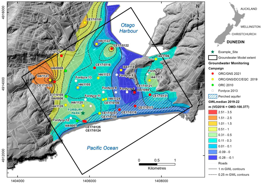
FIGURE 1. Groundwater monitoring sites located within groundwater model extent of South Dunedin. The piezometers used in this study (coloured by installation campaign) are shown with interpolated piezometric surface (updated from Cox et al., 2020). The star indicates the location of the Forbury Park “Example site,” referenced in Section 4 of this paper. The blue shaded area is the interpreted extent of a perched aquifer in the sand dunes. The Otago Metric Datum (OMD) used in this study is equivalent to New Zealand Vertical Datum 2016 (NZVD2016) + 100.377 m.

2.1 The groundwater emergence hazard

A shallow unconfined coastal groundwater system underlies South Dunedin. Groundwater levels are typically found <1 m below the ground surface and there is evidence of some hydraulic connection with the Pacific Ocean (Cox et al., 2020). The expected rise in groundwater levels resulting from SLR must be considered in future land-use and infrastructure planning in South Dunedin.

In the near term, SLR will compound interrelated hazards resulting from the complex interaction between shallow groundwater, buried civil infrastructure and surface waters (e.g., Bell et al., 2017). In the long term, SLR is expected to lead to the emergence of groundwater at the surface (groundwater inundation for the purpose of our research). Hence, central and local government, planners, engineers, and residents are amongst the many concerned by the extent of rising groundwater levels, and the inundation hazard (e.g., PCE, 2015).

2.2 Conceptual model

The latest geological and hydrogeological understanding of South Dunedin is described in detail by Glassey et al. (2003) and Cox et al. (2020) respectively. The current conceptual model of the groundwater system was based on these descriptions.

The topographically flat area represents a valley infilled with Quaternary sediments. The groundwater system flows within two sediment depositional units: 1) a younger Holocene unit comprising soft silt and clay of marine to estuarine origin, locally deposited during the post-glacial marine transgressions resulting from Holocene sealevel rise, overlying 2) a Pleistocene depositional unit comprising sands, silts, and some gravels, interpreted as alluvial deposits with hillslope deposits at the valley margins (colluvium). These highly heterogeneous Pleistocene and Holocene sediments have a maximum depth of approximately 60 m. The contact between the Quaternary sediments and the underlying bedrock is relatively flat beneath most of South Dunedin, but has some (<40 m relief) paleo-topography (Glassey et al., 2003). Bedrock comprises either weak marine sedimentary rock (Caversham sandstone), or a variety of local interbedded igneous rocks (Dunedin Volcanic Group).

The groundwater system was treated conceptually as a single groundwater system for the purposes of this study, being bounded by basement rocks of the Dunedin Hills and Otago Peninsula, and the Pacific Ocean and Otago Harbour (Figure 1). The bedrock contact was treated as a no-flow boundary because recent investigations indicated negligible vertical hydraulic gradients (Cox et al., 2020), and limited vertical groundwater flow at the basin scale (Rekker, 2021).

In contrast to the underlying shallow unconfined groundwater system, a minor perched dune aquifer system to the south (Figure 1) demonstrates low electrical conductivity (i.e., relatively fresh composition) and the absence of a tidal signal (Cox et al., 2020). Unlike many other coastal areas in eastern New Zealand (e.g., Christchurch), there is no evidence to date which suggests any compartmentalisation by distinct inter-glacial aquitards, and the groundwater system lacks any deep groundwater at artesian pressures (e.g., Cox et al., 2021). Our conceptual model therefore assumes minimal “cross-boundary” interaction with other aquifers (e.g., the minor perched dune system to the south) and limited surface inflows from the surrounding catchments.

A streamline no-flow boundary was added along the northern boundary, separating the South Dunedin groundwater system from that of Harbourside, along a catchment and stormwater runoff boundary across the coastal plain (Figure 1). This assumption was justified because groundwater appears to flow approximately parallel to the boundary within coastal sediments.

2.2.1 Groundwater mass flow balance

As is typical of urban centres, surface hydrology is heavily modified and groundwater recharge is highly variable. The impervious land surface within the region causes approximately 60% of precipitation to be captured and routed via the stormwater network, mainly discharging to the Otago Harbour via the pumping station (Goldsmith and Hornblow, 2016). The remainder is available for groundwater recharge via pervious surfaces.

Potential groundwater recharge is relatively well constrained. A weather station within the modelled domain indicates an annual-average precipitation rate of 674 mm/yr between 1997 and 2021. The available stormwater pumping and precipitation data, combined with the imperviousness index for South Dunedin, indirectly leads to a recharge estimate of ∼4,000 m³/day.

Some of this groundwater then exits the system via infiltration to the ageing waste and stormwater networks, which is estimated at 2,000 m³/day (Opus and URS, 2011a; Opus and URS, 2011b; Rekker, 2012; Fordyce, 2013; Cox et al., 2020). The spatial and temporal distribution of groundwater infiltration to the networks remains highly uncertain (Cox et al., 2020). The remainder leaves the system as submarine groundwater discharge. Offshore groundwater discharge and the geology which controls it, remains largely unknown. However, it is constrained by the difference in these mass balance recharge and drainage network estimates.

2.3 Groundwater level monitoring

There is a recent and extensive record of piezometric levels across South Dunedin (Figure 1). Automated meters currently record groundwater levels in 28 piezometers every 15 min within the modelled domain. These were installed over various field campaigns from 2010 to 2021 (see Cox et al., 2020 for a detailed description of the groundwater monitoring network and data coverage).

The interpolated median groundwater piezometric contours suggest that groundwater flows to the Pacific Ocean and Otago Harbour, as shown in Figure 1 (updated from Cox et al., 2020). Median groundwater levels are on average above mean sea-level, with the highest levels occurring in the north-western corner of the system.

Fluctuations in groundwater levels are nearly all restricted to <1 m in range, and dominated by short term variability linked to frontal rain systems, with some cyclicity at a 90–100 day period that reflects cumulative rainfall and recharge caused by the frequency of cyclonic storms (Cox et al., 2020). Any seasonal (e.g., summer vs. winter, or autumn vs. spring) cyclicity, or interannual variability over the decadal period of monitoring to date has been limited, making it relatively robust to use average levels for the steady-state approximation used for history matching (see Section 3).

The tidal range at the harbour/coast is approximately 1.7 m (see Supplementary Figure S1-1). Tidal fluctuations are recorded at some monitoring locations. For example, the groundwater level time series for piezometer I44/0007 (location shown in Figure 1) demonstrates a characteristic diminished amplitude and delayed arrival of the tidal signal (see Supplementary Figure S1-1). The groundwater time series at I44/0007 demonstrates a tidal range of approximately 0.3 m (a difference of 1.4 m at a distance of 120 m from the coast) with a lag in the peak of the tidal cycle of 131 min. This site is one of a few with a relatively strong tidal signal (Cox et al., 2020), but elsewhere hydraulic connection with the Pacific Ocean is still evident >1 km from the shore (see hydrographs for I44/0007 and CE17/0105 in Supplementary Figure S1-1, these piezometer locations are shown in Figure 1). Groundwater electrical conductivity and geochemistry suggest most of the groundwater is fresh and there is limited saline intrusion (<10% at 1 km from the shoreline, see Cox et al., 2020; Rekker, 2021).

2.4 Groundwater model

2.4.1 Model structure

The original numerical groundwater flow model was constructed by Rekker (2012) and modified for the purpose of this research (as described below). MODFLOW-NWT (Niswonger et al., 2011) was used to simulate constant-density groundwater flow under both steady-state and transient conditions. The finite-difference grid is a single-layer (representing Holocene and Pleistocene sediments) comprising 90 rows and 80 columns of uniform 40 × 40 m horizontal discretization. The boundary conditions and recharge array for the model are depicted in Figure 2.

FIGURE 2

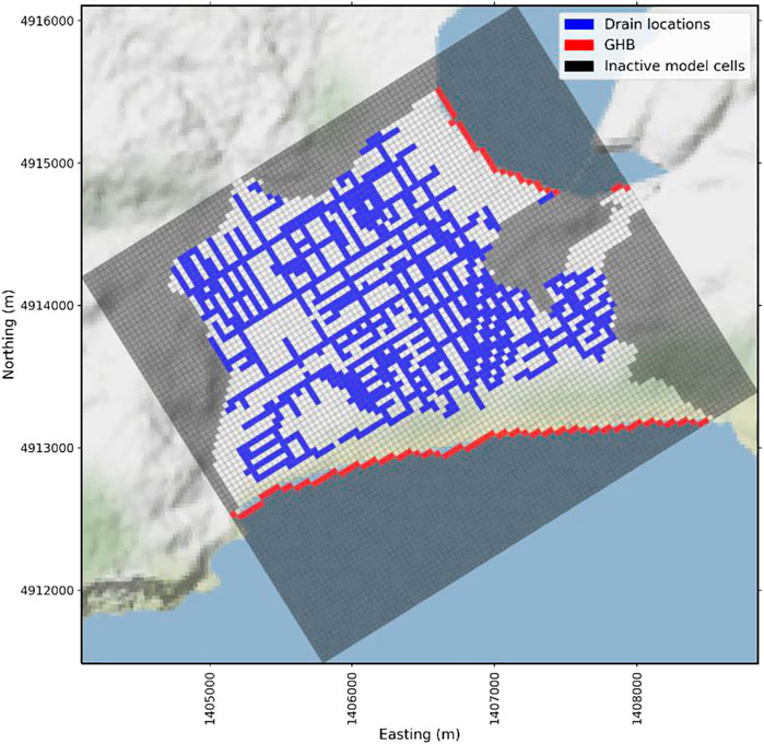
FIGURE 2. South Dunedin model extent showing model grid, boundary conditions and inactive model cells.

The distribution of hydraulic properties was informed by Glassey et al. (2003). The model surface elevations were based on a digital elevation model informed by LiDAR data (1 m digital surface model pixels at specified vertical accuracy <0.2 m, 95% confidence) for South Dunedin (LINZ, 2021). We resampled the LiDAR data to obtain a regridded 40 × 40 m average for the model top elevation of the MODFLOW model domain. The original model bottom elevations estimated by Rekker (2012) from geophysical data, were maintained.

Recharge to the saturated zone is simulated using the MODFLOW recharge (RCH) package. The Otago Harbour and Pacific Ocean were simulated via the General-Head Boundary (GHB) package, and groundwater interaction with the stormwater and wastewater networks is simulated via the MODFLOW Drain (DRN) package (both head-dependent flux packages). The model bottom and other lateral boundaries are “no-flow” boundaries.

Hence, groundwater leaves the model domain as storm/wastewater flow (DRN package), or as submarine groundwater discharge (GHB package). The locations and invert elevations of the stormwater and wastewater networks was informed by city council GIS records. The stormwater network overlies the wastewater network. The surveyed sump elevations for the stormwater network were used in preference over the wastewater network to generate a network of drain locations and elevations within the model domain. That is, the storm and wastewater networks are not separated in our modelling approach. This representation of the storm and wastewater networks is adopted to account for the uncertainty in the conductance and elevation of both drainage networks in our modelling approach (see Section 3).

2.4.2 Temporal discretization

Simulations are divided into a steady-state “history” matching period, with stresses represented by long term average conditions for the period 2010–2020, and a transient “projection” period which simulates system response to IPCC-SLR projections for the period January 2010–January 2110. The density-corrected GHB stage for the history period is specified according to time-averaged tidal data for Port Otago obtained from the New Zealand Hydrographic Authority (Land Information New Zealand, LINZ).

Initial conditions for the transient projection period are established by the steady-state history matching period. The 100-year projection period that follows is discretised into annual stress-periods, and both simulation periods use the same time-invariant (static) properties of hydraulic conductivity, storage, GHB conductance, DRN conductance and DRN elevation. Time-variant properties of recharge and GHB stage are expressed for the projection period. Our approach then focuses on predicting groundwater levels and drain flows under changing GHB (rising sea levels) and recharge (climate variability) model boundary conditions, defined for the projection period.

3 Methodology

This section describes the methodological detail required to implement our approach, including the prediction specification, the development of the parameterisation scheme, history matching and uncertainty quantification. The scripted workflow is provided as a Jupyter Notebook to ensure transparency and reproducibility of the decision-support modelling described herein (Kluyver et al., 2016).

The workflow involves four main components: 1) early uncertainty quantification to assess prior parameter uncertainty and corresponding prediction uncertainty, to identify and resolve inadequacies in the conceptual model or numerical implementation, 2) history matching to condition model parameters that are pertinent to the predictions of interest, 3) Monte Carlo sampling of climate change and SLR parameters in the projection period to explore history matching informed predictive distributions of groundwater levels and, 4) the production of maps assessing the susceptibility to groundwater inundation, and quantification of drain flows under different SLR scenarios. We now describe our approach in detail.

3.1 Model parameterization

Model parameters were defined for both the history and the projection periods. During history matching the following parameters were adjusted: horizontal hydraulic conductivity, history period recharge, GHB conductance, drain conductance, and drain elevation. The additional parameters defined for the projection period comprised: specific yield, specific storage, temporal GHB stage, and temporal recharge (Table 1). Parameters added to the projection period remained unconditioned.

TABLE 1

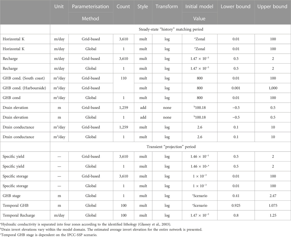
TABLE 1. Parameters and their distribution bounds. “Initial model value” refers to the native model parameter value (units also provided) to which the multiplier (or additive) parameter is applied.

3.1.1 History matching parameters

The distribution of groundwater model hydraulic parameters, flux and head boundary conditions and recharge stresses are expressed through 9855 adjustable parameters for the steady-state history matching period (Table 1). Parameters are generally implemented as multi-scale multipliers which act upon initial model parameter values. Drain elevation parameters are represented as additive, rather than multiplier, parameters. For these, the parameters are applied as an addition or subtraction to the model drain invert elevation estimate.

Parameter operating scales reflect the expected scales of heterogeneity and uncertainty of model input values and are applied at the scale of geological model (global-scale) and the model cell (grid-scale) (e.g., White et al., 2020; Hemmings et al., 2020; McKenna et al., 2020). Initial parameter values, and the mean of their prior distributions, are one and zero, for multiplier and addition parameters, respectively (Table 1).

The prior parameter covariance matrix, from which the prior parameter realisations are drawn, is defined as a block-diagonal matrix. Diagonal elements of the prior parameter covariance matrix represent individual parameter variances, informed by prior, or “expert” knowledge of these model inputs (Table 1). Off-diagonal elements of the covariance matrix, were defined by geostructures built on exponential variograms with sills proportional to the prior parameter variances.

Upper and lower parameter bounds represent a six standard deviation envelope (±3 σ) around the mean of the distributions, equating to approximately a 99% confidence interval. An exponential variogram range of 1,200 m (range a = 400 m) was defined for spatially distributed parameters. However, to account for the anticipated high spatial variance in the (wastewater and stormwater) drainage infrastructure, the exponential variogram range for drain parameters (DRN package invert elevation and conductance) were reduced to 300 m (a = 100 m). Additionally, conservative prior uncertainties were assigned to abstract parameters representing boundary conditions of the structurally simple model (i.e., DRN and GHB conductance). This strategy was employed for uninformed prior uncertainties to avoid under-estimation of predictive uncertainty (e.g., Hugman and Doherty, 2022).

3.1.2 Projection period parameters

An additional 7,423 adjustable parameters were defined for the transient projection period (i.e., 17,276 parameters in total) to represent IPCC projection uncertainty (Table 1). IPCC projections for South Dunedin indicate minimal changes to annual average rainfall rates (e.g., Mourot et al., 2022). However, to represent interannual recharge variability and its uncertainty over the projection period, additional, independent (i.e., no temporal covariance) annual recharge multipliers were included in the analysis.

The initial model input recharge parameter values were estimated from long-term, annual average conditions for the steady-state history period (i.e., a 10-year timeframe). Upper and lower bounds for the temporal recharge multiplier (projection period) were informed by the variance of the 10-year moving average of historic annual rainfall rates. This was based on local long-term New Zealand MetService data for the period 1960–2021 (Table 1). As a consequence, the model is focussed towards predicting the transient progression of long-term annual conditions of groundwater levels, but not short-term (events-based) fluctuations that may be important for managing individual rain-event flood risk.

In contrast to groundwater recharge, projected rises in sea levels are significant, but also highly uncertain during the 21st century and beyond. The modelling workflow uses improved, location specific SLR projections provided by the NZ SeaRise: Te Tai Pari O Aotearoa Endeavour programme. These projections, which can be accessed through https://searise.takiwa.co/, include the effects of vertical land movement for every 2 km of the coast of Aotearoa New Zealand to the year 2,300. Here, to follow coastal planning recommendations specific to New Zealand (MfE, 2017), we focus on SLR projections associated with the IPCC Shared Socioeconomic Pathway (SSP) medium confidence, high emmissions scenario SSP5-8.5. However, the workflow is rapid and easily adaptable to explore any of the SLR scenarios, so we present an additional scenario in the Supplementary Information.

SLR projection uncertainty was propagated through the groundwater model to the predictions of interest according to the defined uncertainty interval for the IPCC-SSP scenario (SSP5-8.5 medium confidence; inferred from Table 2, where p17-p83 is assumed to encompass 2 σ). This SLR scenario uncertainty is represented through the variance on a global (spatially and temporally constant) multiplier, which acts on the median SLR projection timeseries (implemented through the GHB stage) applied across all stress periods. For SSP5-8.5 (Table 2), the variance of this global multiplier, with a mean of 1.0, was defined as 0.12 (standard deviation of 0.34). Also note, the potential range of the forcing applied to the GHB stage increases into the future as the uncertainty of the SLR scenario increases (i.e., heteroscedasticity). The resulting sampled projection period realisations of SLR for the SSP5-8.5 (medium confidence) scenario are illustrated in Figure 3.

TABLE 2

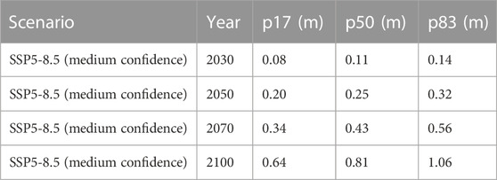
TABLE 2. Relative-SLR projections for South Dunedin (https://searise.takiwa.co/) showing median (p50), 17th percentile (p17) and 83rd percentile projections for the SSP-8.5 (medium confidence) scenario. The realized ensemble of SLR projections drawn from this scenario are shown in Figure 3.

FIGURE 3

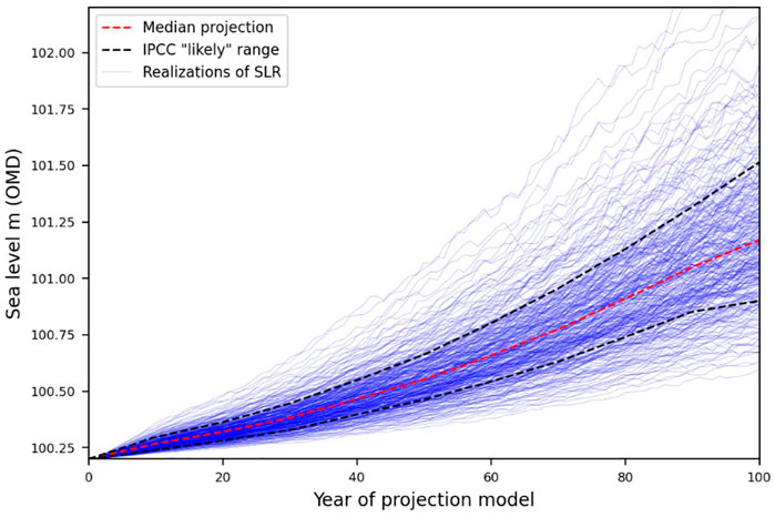
FIGURE 3. Realizations of sea level rise attached to the GHB stage of the 100-year projection model (2010–2110). The plot shows 300 realizations of sea level rise for the IPCC SSP5-8.5 (medium confidence) scenario.

Inter-annual variability and uncertainty for each individual SLR realization is defined through annual multipliers sampled within a ±3 σ range of 0.925–1.075, and covariance defined through a temporal exponential variogram with a range of 15 years (range a = 5 years). This choice was informed by a variogram analysis of the detrended annual average sea level recorded at the Green Island tide gauge (Bell et al., 2022).

Appending SLR parameters to the model parameter covariances supports drawing realisations for the projection period, thus allowing the ensemble of realisations to characterise the embedded deep uncertainty of future SLR projections (e.g., Kopp et al., 2019), and their impact on the decision-critical prediction. To the best of the authors’ knowledge, the explicit application of IPCC-SSP SLR scenario uncertainty to probabilistic groundwater flow model predictions, remains unexplored.

3.2 History matching, uncertainty quantification, and predictions

A prior-based Monte-Carlo uncertainty analysis was used to assess the credibility of the model structure and the prior parameter probability distributions, via observations of prior-data conflict (e.g., Egidi et al., 2022). History matching was then used to derive the posterior parameter ensemble, based on observations from the “history” period, using the iterative Ensemble Smoother (iES) in PEST++ (White, 2018). We then analysed the extent to which history matching (to the available data) was able to refine the distributions of parameter values, their combinations, and the corresponding predictions of interest.

Predictive scenarios, which include additional SLR and recharge uncertainty in the 2010–2110 projection period, were then simulated. This was achieved by combining the posterior parameter ensemble (for the history period) with additional unconditioned parameters relating only to the 100-year projection period (i.e., temporal GHB stage and recharge parameters, see Table 1). The resulting history matching informed parameter ensemble represents the conditioned uncertainty of groundwater levels in response to IPCC-SSP scenarios. These spatially distributed groundwater level predictions can then be used to map the potential SLR-driven groundwater inundation hazard in South Dunedin, supporting risk-based decision making.

3.2.1 Geostatistical draws, observations, and weights

An ensemble of 300 parameter realisations, providing a representation of prior parameter uncertainty, were drawn by Monte-Carlo multi-variate Gaussian sampling of the prior parameter covariance matrix, and then conditioned through history matching. These 300 parameter realizations were ultimately propagated through to the SLR scenario projection period.

The choice of the number of realisations (to propagate through the analysis) is a trade-off between minimising computational burden of the history matching process, whilst endeavouring to sufficiently capture prediction uncertainty, and accommodate the dimensionality of the solution space (e.g., Knowling et al., 2019; White et al., 2020; Hunt et al., 2021). To ensure that 300 realisations appropriately captured the prediction uncertainty, we preformed a convergence analysis, focussing on four prediciton locations of interest. The results of this convergence analysis are shown in Supplementary Figure S3-5. The converenge analysis indicates that 300 realisations effectively captures the prior prediction distribution behaviour (ensemble mean, standard deviation and 95th percentile) represented by 1,000 realisations.

The history matching dataset comprised of long-term averages of system observations. Groundwater level observations were separated into two groups relating to the duration of the piezometer dataset (Table 3). An additional estimate of the annual average total groundwater-waste/stormwater exchange flux of 2,000 m³/day was included as a target observation for history matching (Opus and URS, 2011a; Opus and URS, 2011b; Rekker, 2012; Fordyce, 2014).

TABLE 3

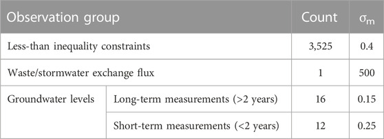
TABLE 3. Measurement error (standard deviation, σ_m).

Given the spatial sparsity of groundwater level measurements, it was beneficial to include observations which represent physically “realistic” constraints on simulated groundwater levels for the history matching period. This was implemented through the “less-than” inequality constraint (White, 2018). Less-than inequality observations contribute to the objective function only when the simulated value exceeds the observation value.

For our purposes, less-than observations were defined for simulated heads in every model cell. The observation value was set according to the model top elevation in the corresponding cell. This effectively implements a history matching constraint, which enforces the condition that long-term average groundwater levels should fall below the model top elevation (e.g., White, 2018; White et al., 2019; Fienen et al., 2021).

Initial observation weights were defined to reflect the estimated observation error. Weights were then re-adjusted to direct parameter upgrades towards objective function components that were considered most relevant to the decision-support objective (e.g., Doherty and Welter, 2010; Fienen et al., 2022). In particular, because groundwater level observations used for history matching are well “aligned” with the decision-critical prediction, these were assigned a greater weight (e.g., Dausman et al., 2010; Knowling et al., 2019; Fienen et al., 2020). This was achieved by scaling the inequality and groundwater-waste/stormwater flux observation group weights by 1 × 10⁻¹.

4 Results and discussion

The main outputs of this research are hazard informed maps for decision support. We therefore begin our examination of the results with this aspect of the study. We then discuss projected drainage volumes. This is followed by examining the value of history matching (e.g., Doherty and Moore, 2017), and the use of ‘difference from a baseline,’ or comparative outcomes of model predictions as an alternative approach, when investigating the SLR-driven groundwater hazard (e.g., Sepúlveda and Doherty, 2015).

The IPCC AR6 report introduced the SSP scenarios, which are representative of a broad range of plausible societal and climatic futures (IPCC, 2021). As detailed above, the focus of this research is the presented framework/workflow, so we mainly discuss results for the recommended SSP5-8.5 (medium confidence) high emissions scenario (MfE, 2017; see Table 2; Figure 3). However, we also briefly discuss and compare results for the SSP2-4.5 (medium confidence) scenario, which is included in the Supplementary Information.

4.1 Projected probability of groundwater inundation

To explore predictive uncertainty under IPCC projections of SLR, the estimated probability (and thus susceptibility) to groundwater inundation was based on a history matched (posterior) parameter ensemble. This posterior was derived using a Monte-Carlo representation of parameter uncertainty, that was propagated to the SLR projection period. The resulting probability of groundwater inundation was estimated from the posterior groundwater level distributions at every model cell, and collating the number of occasions that groundwater levels exceeded the model top elevation (i.e., exceedance probability, Figure 5). For the purposes of our research, susceptibility to inundation and probability are on the same general scale: highly susceptible areas correspond to the highest probabilities of groundwater levels exceeding the model top, and vice versa.

Using the SSP5-8.5 projection, the model simulated groundwater levels prior to 2030, indicate that the simulated probability of groundwater inundation is generally low across the South Dunedin model domain. This is likely associated with the low to moderate SLR projection and relatively constrained SLR uncertainty for this timeframe (Figure 3). By 2030, regions of higher groundwater inundation probability begin to emerge (Figure 4A). These regions become more defined by 2050 (Figure 4B) and are broadly constrained to three zones, in low-lying areas, surrounding the example site, I44/0006 and I44/1113 (Figure 1). This is consistent with reports of depths to groundwater of <0.5 m below the ground surface in these areas (Cox et al., 2020). It is not surprising, therefore, that these low-lying regions would be susceptible to inundation for low to moderate rises in sea level.

FIGURE 4

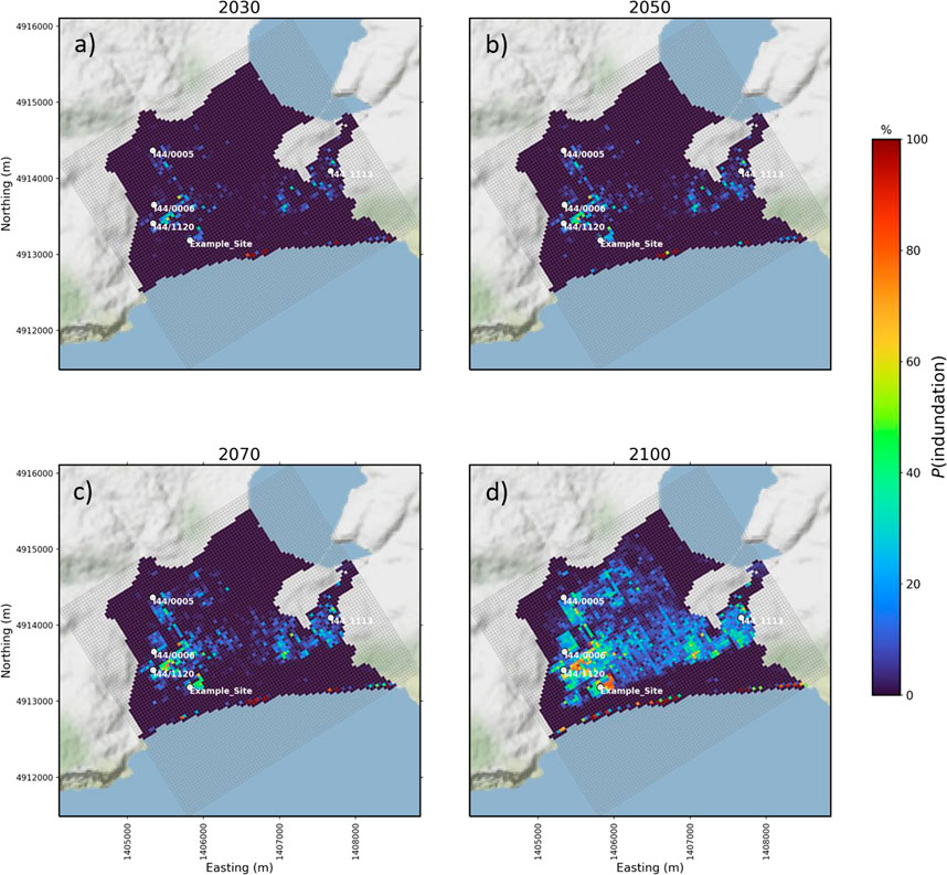
FIGURE 4. The projected SLR-driven probability of groundwater inundation for 2030, 2050, 2070 and 2100 based on the IPCC SSP5-8.5 (medium confidence) scenario (see Figure 3 for realizations of relative-SLR attached to GHB stage in the model). The model top elevation is based on a Digital Elevation Model (DEM) informed by recent LiDAR data (LINZ, 2021).

Under increasing (and accelerating) SLR for the 2070–2100 timeframe, the spatial extent of the more susceptible areas continues to increase (Figures 4C, D). As expected, the regions with the highest inundation probabilities are dominated by the same low-lying open areas, especially where there is an absence of drainage in the model (e.g., in the region of I44/0006, Figure 4). However, many additional zones do appear susceptible to the inundation hazard, despite being >1 m above sea level and a considerable distance inshore (e.g., in the region of I44/0005, Figure 4).

These same broad trends are apparent for the SSP2-4.5 (medium confidence) scenario. Although, the simulated probability and spatial extent of groundwater inundation is slightly diminished for the 2070–2100 timeframe (see Supplementary Figure S4-1). We attribute this reduction in susceptibility to the lower SLR projection attached to the model boundary condition for the SSP2-4.5 (medium confidence) scenario (see Supplementary Figure S4-2). Importantly, the lower likelihood high SLR realisations captured by our modelling approach leads to elevated probabilities of groundwater inundation for this timeframe. Our results suggest that even for the more optimistic SSP2-4.5 emissions pathway, significant susceptibility to the groundwater indundation hazard remains.

The zones most prone to groundwater inundation are not correlated with the distance from the Pacific Ocean or Otago Harbour boundary conditions (Figure 4). We hypothesize that this may be related to the increased hydraulic conductivity of the sediments and low topographic relief of these areas. Our results imply that groundwater emergence at a considerable distance inshore may occur before, or even compound overland flooding (e.g., Befus et al., 2020; Plane et al., 2019). This has implications for adaptation strategies that focus solely on overland flooding. Ignoring the effects of SLR-driven groundwater level rises may significantly underestimate the spatial extent and timing of surface water flooding (e.g., Anderson et al., 2018).

The presented inundation probabilities are all relative to the model top elevation (Figure 4), estimated from a mean aggregation of the LiDAR data (Section 2). It is acknowledged that the uncertainty of the LiDAR data, and how it is aggregated to the model top, has not been explicitly addressed in this study. A strong correlation is likely to exist between model surface elevation and simulated water levels. We believe that our framing of water level predictions as relative to the model top will help mitigate potential elevation and aggregation errors. However, caution should be exercised when attempting to assess inundation probabilities at scales less than the model grid resolution. Small-scale topographic features within a model cell may be characterised by higher (or lower) inundation probabilities than those predicted, at the model grid scale relative to the model top. The impact of elevation and aggregation uncertainty on predictions of groundwater inundation at a finer scale could be addressed in future work.

4.2 Simulated drain flows

The projected SLR-driven probability and spatial extent of inundation (Figure 4) is mitigated by the interaction between rising groundwater levels and the waste/stormwater drainage networks. This mitigating effect is controlled by the relative elevation of groundwater levels as sea levels rise, and also the spatial conductance of the drainage networks (an abstract numerical representation of the complex interaction between groundwater and the drainage networks, Table 1).

This effect is demonstrated by the total flux of groundwater discharging to the drainage networks represented in the model of South Dunedin, which is projected to increase substantially (Figure 5). As with the groundwater level predictions, the uncertainty of the total drain flux prediction also increases over the duration of the projection scenario (Figure 5). For example, in 2030, the mean and standard deviation of drainage flows are 2,150 and 494 m³/day, respectively. In 2100, this increases to 2,835 and 718 m³/day, respectively (a 32% increase in projected mean drainage flows).

FIGURE 5

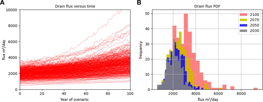
FIGURE 5. Plots showing (A) time-series of individual realizations of total drain fluxes, and (B) Probability Density Functions (PDFs) of projected total drain fluxes as groundwater levels change [IPCC SSP5-8.5 (medium confidence) scenario]. These plots show the estimated total groundwater flux to the waste/stormwater networks represented in the model of South Dunedin.

Drain conductance and elevation are expressed as (nested) uncertain parameters in the numerical modelling workflow presented herein, but the history matching results indicate that the available data provides little information for condition of these parameters, especially in a spatial sense (see Supplementary Figure S3-7). Significant uncertainty persists for these posterior predictions. Additional monitoring, data collection and refinement of the estimated spatial (and temporal) fluxes to the existing drainage network may help reduce the uncertainty of these (and other) parameters, and thereby help to reduce the uncertainty of both drain flux and groundwater inundation predictions.

Notwithstanding the large uncertainty of these predictions, our results are consistent with other recent studies (e.g., Habel et al., 2017; Befus et al., 2020), which suggest that drainage may offset the impacts of SLR and emergent groundwaters. However, the planned renewal of the waste and stormwater networks in the 2020–2050 timeframe (Goldsmith and Hornblow, 2016) may limit, or even reduce the capacity of the drainage networks to accept infiltrating groundwater.

This has profound implications for decision-makers in South Dunedin, since our approach conservatively assumes that the drainage system will be available to accommodate SLR-driven groundwater level rises (Figure 5). This tenuous (linear) assumption may significantly overestimate the hydraulic response of the waste/stormwater networks for conditions that may prevail in the future. Decision-makers should therefore consider potential future limitations, or reductions of drainage flows in future management scenarios, to avoid underestimation of the potential groundwater inundation hazard.

The projected SLR-driven increase in the base flux to the waste/stormwater networks (Figure 5) will also be an important consideration. Increased “dry condition” flows to the drainage networks might limit their capacity for their primary function (removal of wastewater and stormwater, e.g., Morris et al., 2018). This has significant implications for managing event flows, since increases in the base flux may compound rises in groundwater levels in response to these events. Where the flows to these networks requires treatment and pumping to discharge, as is the case in South Dunedin, treatment facilities will likely receive higher loads at significant extra cost with ramifications for facility downtime and failure (e.g., Cox et al., 2020).

4.3 The value of history matching

The simulated outputs from the prior-based Monte Carlo uncertainty quantification displayed minimal prior-data conflict (PDC) in relation to the predictions of interest (groundwater levels; see Supplementary Figure S3-9). That is, prior simulated output distributions generally encompass the values of system observations. However, the prior uncertainty of simulated outputs was significant and contributed to predictions of relatively high probability of inundation (during the history period), across the model domain (Supplementary Figure S3-1). This high uncertainty in simulated outputs of management interest, the availability of aligned observations, and the general lack of PDC provided a defensible basis for undertaking history matching.

Six iterations using the iES algorithm were used to history match simulated outputs to historical observations (Section 3.2). This required a total of 3,240 model runs. The match to long-term average groundwater levels and total drain flux improved significantly in the first two iterations and levelled off following the fourth (Supplementary Table S3-1). After history matching, the posterior simulated groundwater level distributions generally encompass their respective observation within the defined observation error. The prior and posterior Probability Density Functions (PDFs) for three observation locations, and an additional example site, are provided in Figure 6 (distributions for all observations are shown in Supplementary Figure S3-9).

FIGURE 6

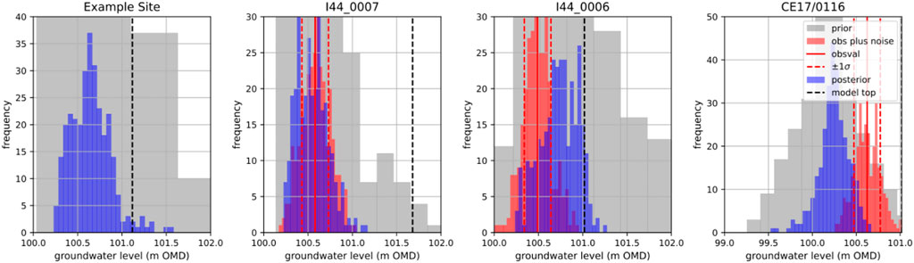
FIGURE 6. Histograms (PDFs) for selected observations showing prior Monte Carlo, posterior and observation plus noise iES distributions. Blue histograms show the distribution of model outputs and red histograms show the realizations of the observation value, which is based on the observed long-term (mean) groundwater level and supplied standard deviation (i.e., σ_m). Note, the unweighted example site for which no observation exists (Example Site). Note also, the x-range is truncated to focus on the posterior model outputs (history period).

As expected, history matching to several thousand observations (groundwater levels, inequality constraints and total groundwater flux) significantly reduced the uncertainty of simulated groundwater level predictions, as indicated by the widths of the respective prior and posteriors PDFs in Figure 6 and Supplementary Figure S3-9. Through history matching, the simulated probability of groundwater inundation for the history period, was reduced to 0% across most of the model domain (see Supplementary Figure S3-8). We mainly attribute this improvement to the conditioning of horizontal hydraulic conductivity and drain conductance parameters through the assimilation of the information contained within the observation dataset (Supplementary Figure S3-4).

The history matching process outcome, i.e., the posterior parameter ensemble, can be considered to be effective, since the parameter ensemble was updated by the assimilation of information from observation data. It can also be concluded that these data were suitable for reducing the uncertainty of parameters to which the predictions were sensitive (Supplementary Figure S3-6).

However, results from both the history and projection periods, depict a high spatial and temporal variation in the uncertainty reduction of the groundwater level simulated output that results from history matching (Figure 7 and Supplementary Figure S3-6). The spatial distribution of observation data, the updated impervious surface recharge model (Supplementary Figure S2-1), and simulated drainage clearly plays an important role in the spatial distribution of uncertainty reduction. For example, generally, the largest uncertainty reductions occur over pervious surfaces where the observation density is high, and where there is absence of drainage in the model (e.g., to the southwest of the model domain).

FIGURE 7

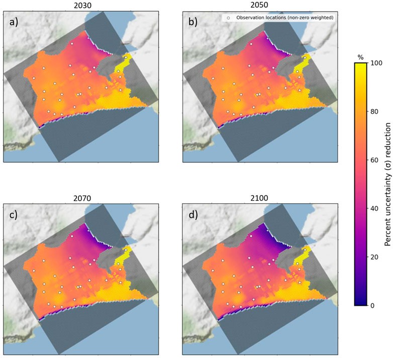
FIGURE 7. Percent uncertainty change for posterior versus prior distributions of groundwater level predictions for (A) 2030, (B) 2050, (C) 2070 and (D) 2100. Observation locations used for history matching are also shown (i.e., non-zero weighted groundwater level observations).

Uncertainty reductions are generally high (>60%) for the history period (Supplementary Figure S3-6) and for the projected 2030–2050 timeframe (Figures 7A, B). As discussed, the conditioning of parameters to historical observations propagated this uncertainty reduction to the projection period groundwater level predictions. Before 2050, our results suggest that steady-state only history matching can indeed reduce the uncertainty of groundwater level predictions, despite the intractable nature of the uncertainty inherited from the IPCC projections of SLR (e.g., Kopp et al., 2019).

Generally, however, posterior prediction uncertainty increases substantially for the 2070–2100 timeframe (Figures 7C, D). Spatially, the history matching constrained uncertainty increases are mainly isolated to locations where drainage is represented in the model, and to the northeast of the model domain where groundwater level observation data is sparse (i.e., near the harbour boundary condition). For the groundwater level prediction, we mainly attribute this loss in spatial confidence to the large uncertainty of the drainage parameters, and the uncertainty inherited from the IPCC-SLR projection, which increases precipitously for the 2070–2100 timeframe (see, e.g., Figure 3).

In this context, groundwater inundation assessments typically rely on the use of a single deterministic realisation of SLR (e.g., median or p83 scenario, see Table 2). Unfortunately, these approaches eschew the deep uncertainty attached to the IPCC-SLR projections themselves (e.g., Kopp et al., 2019), and do not allow expert knowledge to be considered through weighting the likelihood of SLR over the full range of scenario projections (e.g., Purvis et al., 2008). We have therefore presented a consistent methodology to explore the full range of SLR projections and their impact on the decision-critical predictions (see, e.g., Figure 7).

4.4 Predictions of relative change (i.e., differences)

The availability of appropriate groundwater monitoring datasets, particularly at the spatial density and duration of the results presented herein, is relatively rare, especially compared to the global number of at-risk, coastal communities and ecosytems (e.g., Neumann et al., 2015; Hooijer and Verminnen, 2021). For predictions of absolute groundwater levels and inundation, a lack of monitoring data may limit the potential for history matching to condition (and reduce) model parameter and corresponding prediction uncertainty. Our results suggest that the prior uncertainty of these absolute predictions may be too high to provide any meaningful information in terms of robust decision-support (see Supplementary Figure S4-2).

A considered reframing of the projection simulations, to predict the relative changes of model predictions (i.e., differences in projected groundwater levels, Figure 8) may, in practice, be a better approach for communities that do not have dense monitoring networks. Such an approach should reduce the impact of model structural errors on predictive uncertainty, and may also help to mitigate the contribution to uncertainty inherited from the prior parameter distributions and structural defects of the groundwater model (e.g., Sepúlveda and Doherty, 2015).

FIGURE 8

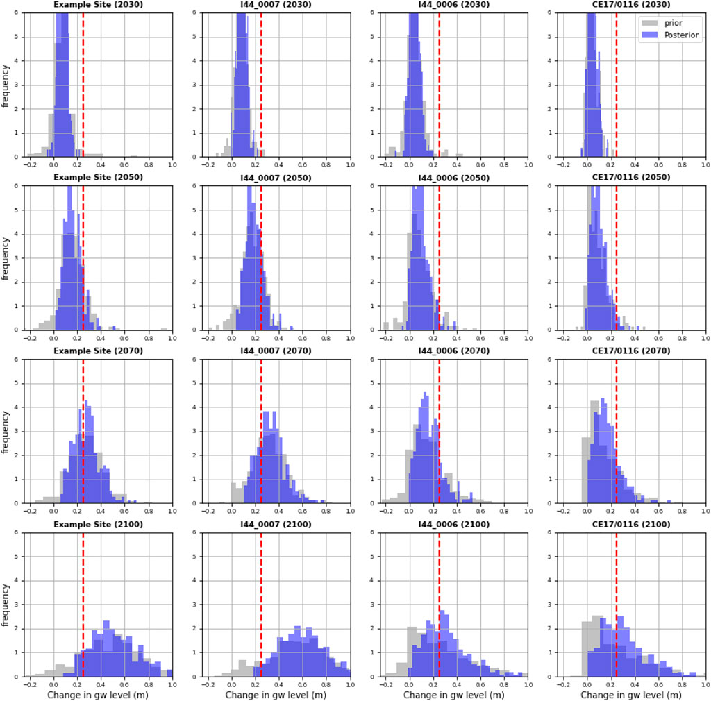
FIGURE 8. Prior (grey) versus posterior (blue) distributions for the projected change in groundwater levels (m) at the selected sites for the SSP5-8.5 (medium confidence) scenario. An arbitrary decision threshold of 0.25 m is also illustrated (red dashed line). The projected change in groundwater levels is calculated from the difference between year 0 and the given year of the projection model (for each individual realization).

The results presented in Figure 4 display the distribution of changes in groundwater levels relative to an arbitrary “decision threshold” (e.g., Knowling et al., 2019; White et al., 2019), which in this instance is emergence over the model top (or land surface) estimated from LiDAR data. Clearly, for relative-type predictions, such a decision threshold is not available. An alternative is to define a threshold based on an anticipated impactful change in groundwater levels. For example, Figure 8 uses a decision threshold of a 0.25 m increase in groundwater levels (for the same sites presented in Figure 6). Probabilistic mapping of simulated outputs against this (or multiple) relative decision thresholds is also possible.

For predictions of relative change, the projected prior versus posterior probability of groundwater levels exceeding the decision threshold appears relatively low for the 2030–2050 timeframe (Figure 8). Similar to the predictions of absolute values, there is then a marked increase in the probability of groundwater levels exceeding the difference threshold for the 2070–2100 timeframe.

However, in contrast to predictions of absolute values, there is a surprising lack of discrepancy between the prior and posterior difference projections (Figure 8). This is consistent with the accepted logic that models are more suitable predictors of relative change, rather than absolutes (e.g., Sepúlveda and Doherty, 2015), which also aligns with conclusions drawn from a number of other recent studies (e.g., Knowling et al., 2019; White et al., 2020).

Our results indicate that the workflow deployed here for South Dunedin could be modified and deployed with reasonable utility, even in settings with limited (or unreliable data), by curtailing, or forgoing the history matching step, and exploring predictions in a relative sense. It may then be possible to delineate areas that are more susceptible to SLR-driven groundwater level rises, or demonstrate the merits of one management strategy versus another. This has implications for the way in which a numerical model is used for decision-support, and the type of information that decision makers may wish to obtain from numerical models.

4.5 Further considerations and recommendations

The history matching informed predictive distributions of groundwater levels presented herein supports quantification of the uncertainties in groundwater level rise and inundation, for stresses that may prevail in the future. It is acknowledged that the modelling workflow does not capture all of the potential contributing sources to predictive uncertainty. We therefore adopted a highly parameterised approach and defined broad prior parameter uncertainties to provide some protection against prediction uncertainty underestimation. Although, some uncertainties relating to error in model structure and conceptualisation (e.g., Wagener et al., 2021) may persist, unaccounted for.

Consequently, caution should be exercised in the application of these results. As discussed in Section 4.1, it may be inappropriate to apply these results at spatial scales finer than the model grid resolution. Similarly, for temporal scales, the model projections represent the long-term progression of annual conditions to estimate a general “annual” exposure to a hazard, or change in exposure to a hazard. Detailed hazard, vulnerability and damage thresholds also commonly encompass short-term fluctuations and events (e.g., Paulik et al., 2019). The direct application of these results to temporal scales that are finer than the model temporal resolution is also likely to be inappropriate. Nevertheless, the modelling workflow and results presented herein may serve as a basis for making downscaled (both temporally and spatially) predicitions.

A real strength is the scripted nature of our workflow, which facilitates such (follow up) investigations, whilst supporting the incorporation of model revisions and exploration of alternative management (e.g., SSP or drainage) scenarios, in a way that is rapid, reproducible and transparent. The workflow could easily be extended to implement dataworth analyses to establish the value of existing and yet to be collected monitoring data. Or, for example, the cost of exploring (or foregoing) transient history matching in terms of reducing predictive uncertainty at finer temporal scale, in an events based models (e.g., Moore and Doherty, 2005).

In this context, it is recommended that future research should explore predictions of an episodic nature, such as improving model-based predictions of groundwater levels in response to individual storm-surge or rainfall events (e.g., a rainfall event with a return period of 10 years). It would then be possible to begin to address the fundamental question of how these events interact with rising sea levels and a changing climate.

5 Conclusion

The potential for a spatial and temporal detailed map of groundwater inundation probabilities, and corresponding drainage volumes that may be required to mitigate SLR, was investigated in this study. While the mapping of groundwater inundation is discussed in Morris et al. (2018) and others, projecting this mapping into a risk framework has been missing from the literature. The distributed properties that support the risk maps of groundwater inundation in response to SLR extends the recent work of Merchán-Rivera et al. (2022), which also applied a Bayesian framework to the creation of risk maps, but used spatially lumped hydraulic properties. The spatially distributed hydraulic properties adopted in this work enabled a detailed delineation of areas that is not possible using a spatially lumped parameterisation scheme. The Bayesian methodology adopted supports a regional scale delineation of the distribution of groundwater inundation projections.

Our approach has attempted to equip decision-makers with all the necessary information to distinguish where the probability for groundwater inundation is relatively high, and where it is relatively low. This approach also includes providing a level of confidence that a proposed decision threshold will be exceeded, which may necessitate the implementation of a (potentially costly) management strategy. However, knowledge of actual thresholds for damage, and therefore asset vulnerability, appears to be missing from the literature. In this regard, the tolerable probability of groundwater inundation, and how this translates more broadly into risk, remains for decision-makers to determine.

Previous studies on groundwater responses to SLR have focussed on groundwater flooding areas, or the movement of the fresh-salt water interface. However, the mitigation of groundwater flooding, at least initially, is likely to involve consideration of the additional flows that drainage networks may be required to accomodate. This study extends previous work by explicitly focussing on the likelihood of relative increases in drainage flows, given its importance as a management consideration.

The uncertainty of the SLR projections represents a small contribution to the uncertainty of the groundwater flooding probabilities for predictions within the next few decades. As the projections extend further into the future, however, the SLR uncertainty begins to dominate the uncertainty of the groundwater flooding predictions. This highlights the necessity of exploring model uncertainty in the context of the prediction being made (Doherty, 2015). For near-time predictions, history matching appears to reduce the uncertainty of groundwater level rises, whereas the same cannot be said for predictions in the distant future.

Also demonstrated was the relative value of history matching when formulating predictions as a difference from a baseline, rather than the absolute value of a prediction. For the specific predictions and history matching dataset combination explored, the worth of history matching was doubtful when casting the prediction as a difference from a baseline. Whereas history matching was useful if the absolute magnitude of the groundwater level was of concern. This issue was also explored in different contexts in Knowling et al. (2019), Hemmings et al. (2021), Moore and Doherty (2005) and others.

Finally, we note that the analysis described in this paper was supported by a scripted workflow (e.g., White et al., 2020). The combination of a spatially and temporally distributed parameterisation scheme, history matching and uncertainty quantification over a regional scale is complex. This scripted workflow provides a transparent record of the many (unavoidable subjective) decisions made during our modelling process, whilst supporting similar analyses that could easily extend the scripted workflow provided in the Supplementary Information.

Data availability statement

The raw data supporting the conclusion of this article will be made available by the authors, without undue reservation.

Author contributions

LC and BH were responsible for coding of the workflow and analysis of the results. SC and CM supported analysis of the results. MK and KH supported the development of the workflow. FM, PG and JR supported the development of the numerical model. All authors contributed to the writing of the manuscript.

Funding

This research was supported by the NZ SeaRise Endeavour programme, funded by the Ministry of Business, Innovation and Employment (MBIE) contract RTVU1705. This research programme was conducted in collaboration with GNS Science, Victoria University of Wellington (VUW) and NIWA. The case study example development was supported by Otago Regional Council (ORC) and Dunedin City Council (DCC) who monitor groundwater and are cognisant of the many issues impacting their community’s future.

Acknowledgments

We would also like to thank the helpful and constructive reviews provided by two reviewers. These reviews substantially improved the manscript.

Conflict of interest

Author KH was employed by Groundwater Solutions Pty., Ltd. and Author JR was employed by Kōmanawa Solutions Ltd.

The remaining authors declare that the research was conducted in the absence of any commercial or financial relationships that could be construed as a potential conflict of interest.

Publisher’s note

All claims expressed in this article are solely those of the authors and do not necessarily represent those of their affiliated organizations, or those of the publisher, the editors and the reviewers. Any product that may be evaluated in this article, or claim that may be made by its manufacturer, is not guaranteed or endorsed by the publisher.

Supplementary material

The Supplementary Material for this article can be found online at: https://www.frontiersin.org/articles/10.3389/feart.2023.1111065/full#supplementary-material

References

Abboud, J. M., Ryan, M. C., and Osborn, G. D. (2018). Groundwater flooding in a river-connected alluvial aquifer. J. Flood Risk Manag. 11 (4), e12334. doi:10.1111/jfr3.12334

CrossRef Full Text | Google Scholar

Anderson, T. R., Fletcher, C. H., Barbee, M. M., Frazer, L. N., and Romine, B. M. (2015). Doubling of coastal erosion under rising sea level by mid-century in Hawaii. Nat. Hazards 78 (1), 75–103. doi:10.1007/s11069-015-1698-6

CrossRef Full Text | Google Scholar

Anderson, T. R., Fletcher, C. H., Barbee, M. M., Romine, B. M., Lemmo, S., and Delevaux, J. (2018). Modeling multiple sea level rise stresses reveals up to twice the land at risk compared to strictly passive flooding methods. Sci. Rep. 8 (1), 1–14. doi:10.1038/s41598-018-32658-x

PubMed Abstract | CrossRef Full Text | Google Scholar

Barlow, P. M., Wagner, B. J., and Belitz, K. (1996). Pumping strategies for management of a shallow water table: The value of the simulation-optimization approach. Groundwater 34 (2), 305–317. doi:10.1111/j.1745-6584.1996.tb01890.x

CrossRef Full Text | Google Scholar

Befus, K. M., Barnard, P. L., Hoover, D. J., Finzi Hart, J. A., and Voss, C. I. (2020). Increasing threat of coastal groundwater hazards from sea-level rise in California. Nat. Clim. Change 10 (10), 946–952.

CrossRef Full Text | Google Scholar

Bell, R., Hannah, J., and Andrews, C. (2022). Update to 2020 of the annual mean sea level series and trends around New Zealand. Hamilton, New Zealand: Prepared for Ministry for the Environment. August 2022 (NIWA Client Report No: 2021236HN). NIWA. Available at: https://environment.govt.nz/publications/update-to-2020-of-the-annual-mean-sea-level-series-and-trends-around-new-zealand.

Google Scholar

Bell, R., Lawrence, J., Allan, S., Blackett, P., and Stephens, S. (2017). Coastal hazards and climate change: Guidance for local government. Wellington (NZ): Ministry for the Environment, 279.

Google Scholar

Bjerklie, D. M., Mullaney, J. R., Stone, J. R., Skinner, B. J., and Ramlow, M. A. (2012). “Preliminary investigation of the effects of sea-level rise on groundwater levels in New Haven, Connecticut,” in Open-File Report 2012-1025. US Geological Survey (Reston, Virginia: The US Geological Survey).

CrossRef Full Text | Google Scholar

Box, J. E., Hubbard, A., Bahr, D. B., Colgan, W. T., Fettweis, X., Mankoff, K. D., et al. (2022). Greenland ice sheet climate disequilibrium and committed sea-level rise. Nat. Clim. Chang. 12, 808–813. doi:10.1038/s41558-022-01441-2

CrossRef Full Text | Google Scholar

Caers, J. (2018). “Bayesianism in the geosciences,” in Handbook of mathematical geosciences (Fifty Years of IAMG), 527–566. doi:10.1007/978-3-319-78999-6_27

CrossRef Full Text | Google Scholar

Colombo, L., Gattinoni, P., and Scesi, L. (2018). Stochastic modelling of groundwater flow for hazard assessment along the underground infrastructures in Milan (northern Italy). Tunn. Undergr. Space Technol. 79, 110–120. doi:10.1016/j.tust.2018.05.007

CrossRef Full Text | Google Scholar

Cooper, H. M., Fletcher, C. H., Chen, Q., and Barbee, M. M. (2013). Sea-level rise vulnerability mapping for adaptation decisions using LiDAR DEMs. Prog. Phys. Geogr. 37 (6), 745–766. doi:10.1177/0309133313496835

CrossRef Full Text | Google Scholar

Cox, S. C., Ettema, M. H. J., Mager, S. M., Glassey, P. J., Hornblow, S., and Yeo, S. (2020). Dunedin groundwater monitoring and spatial observations. Lower Hutt (NZ). Avalon, Wellington, New Zealand: GNS Science GNS Science, 86. Report 2020/11. doi:10.21420/AVAJ-EE81

CrossRef Full Text | Google Scholar

Cox, S. C., van Ballegooy, S., Rutter, H. K., Harte, D. S., Holden, C., Gulley, A. K., et al. (2021). Can artesian groundwater and earthquake-induced aquifer leakage exacerbate the manifestation of liquefaction? Eng. Geol. 281, 105982. doi:10.1016/j.enggeo.2020.105982

CrossRef Full Text | Google Scholar

Dausman, A. M., Doherty, J., Langevin, C. D., and Sukop, M. C. (2010). Quantifying data worth toward reducing predictive uncertainty Groundwater 48 (5), 729–740.

CrossRef Full Text | Google Scholar

Doherty, J. (2015). Calibration and uncertainty analysis for complex environmental models, 227pp. Brisbane, Australia: Watermark Numerical Computing.

Google Scholar

Doherty, J., and Moore, C. (2017). “Simple is beautiful,” in Moore C. 2019. Groundwater modelling uncertainty – implications for decision making. Summary report of the national groundwater modelling uncertainty workshop, 10 July 2017. Editors H. Middlemis, G. Walker, L. Peeters, S. Richardson, and P. Hayes (Sydney, Australia: Flinders University, National Centre for Groundwater Research and Training). doi:10.25957/5ca5641defe56

CrossRef Full Text | Google Scholar

Doherty, J., and Welter, D. (2010). A short exploration of structural noise. Water Resour. Res. 46 (5).

CrossRef Full Text | Google Scholar

Egidi, L., Pauli, F., and Torelli, N. (2022)., 28. Avoiding prior–data conflict in regression models via mixture priors. Can. J. Stat. 50 (2), 491–510.

CrossRef Full Text | Google Scholar

Fienen, M. N., Corson-Dosch, N. T., White, J. T., Leaf, A. T., and Hunt, R. J. (2022). Risk-based wellhead protection decision support: A repeatable workflow approach. Groundwater 60 (1), 71–86.

CrossRef Full Text | Google Scholar

Freeze, R. A., Massmann, J., Smith, L., Sperling, T., James, B., and Fordyce, E. (1990)., 28. Hydrogeological decision analysis: 1. A framework groundwater 5Groundwater dynamics of a shallow coastal aquifer [MAppSc thesis]. Dunedin (NZ): University of Otago. 155p, 738–766.

CrossRef Full Text | Google Scholar

Fordyce, E. (2014). Groundwater dynamics of a shallow coastal aquifer. (Doctoral dissertation, University of Otago). 155.

Google Scholar

Glassey, P., Barrell, D., Forsyth, J., and Macleod, R. (2003). The geology of Dunedin, New Zealand, and the management of geological hazards. Quat. Int. 103, 23–40. doi:10.1016/S1040-6182(02)00139-8

CrossRef Full Text | Google Scholar

Goldsmith, M., and Hornblow, S. (2016). The natural hazards of South Dunedin. Dunedin, New Zealand: Otago Regional Council Report, Otago Regional Council, 69.

Google Scholar

Goldsmith, M., Payan, J-L., MorrisValentine, R. C., MacLean, S., Xiaofeng, L., Vaitupu, N., et al. (2015). Coastal Otago flooding flood event 3 june 2015. Dunedin (NZ): Otago Regional Council, 56p.

Google Scholar

Habel, S., Fletcher, C. H., Rotzoll, K., and El-Kadi, A. I. (2017). Development of a model to simulate groundwater inundation induced by sea-level rise and high tides in Honolulu, Hawaii. Water Res. 114, 122–134. doi:10.1016/j.watres.2017.02.035

PubMed Abstract | CrossRef Full Text | Google Scholar

Habel, S., Fletcher, C. H., Rotzoll, K., El-Kadi, A. I., and Oki, D. S. (2019). Comparison of a simple hydrostatic and a data-intensive 3D numerical modeling method of simulating sea-level rise induced groundwater inundation for Honolulu, Hawai’i, USA. Environ. Res. Commu-nications 1 (4), 041005. Available at:. doi:10.1088/2515-7620/ab21fe

CrossRef Full Text | Google Scholar

Hall, J. A., Gill, S., Obeysekera, J., Sweet, W., Knuuti, K., and Marburger, J. (2016). Regional Sea level scenarios for coastal risk management: Managing the uncertainty of future Sea Level change and extreme water levels for department of defense coastal sites worldwide. Alexandria: U.S. Department of Defense, Strategic Environmental Research and Development Program.

Google Scholar

Hemmings, B., Knowling, M. J., and Moore, C. R. (2020). Early uncertainty quantification for an improved decision support modeling workflow: A streamflow reliability and water quality example. Front. Earth Sci. 8, 565613. doi:10.3389/feart.2020.565613

CrossRef Full Text | Google Scholar

Hooijer, A., and Verminnen, R. (2021). Global LIDAR land elevation data reveal greatest sea-level rise vulnerability in the tropics. Nat. Commun. 12, 3592–3597. doi:10.1038/s41467-021-23810-9

PubMed Abstract | CrossRef Full Text | Google Scholar

Hoover, D. J., Odigie, K. O., Swarzenski, P. W., and Barnard, P. L. (2016). Sea-level rise and coastal groundwater inundation and shoaling at select sites in California, USA. J. Hydrology Regional Stud. 11, 234–249. doi:10.1016/j.ejrh.2015.12.055

CrossRef Full Text | Google Scholar

Hugman, R., and Doherty, J. (2022). Complex or simple-does a model have to be one or the other? Front. Earth Sci 10, 1–12. doi:10.3389/feart.2022.867379

PubMed Abstract | CrossRef Full Text | Google Scholar

Hunt, R. J., White, J. T., Duncan, L., Haugh, C., and Doherty, J. (2021). Evaluating lower computational burden approaches for calibration of large environmental models. Ground Water 59 (6), 788–798. doi:10.1111/gwat.13106

PubMed Abstract | CrossRef Full Text | Google Scholar

Jevrejeva, S., Grinsted, A., and Moore, J. C. (2009). Anthropogenic forcing dominates sea-level rise since 1850. Geophys. Res. Lett. 36, L20706. doi:10.1029/2009gl040216

CrossRef Full Text | Google Scholar

Kluyver, T., Ragan-Kelley, B., Pérez, F., Granger, B., Bussonnier, M., Frederic, J., et al. (2016). “Jupyter notebooks—a publishing format for reproducible computational workflows,” in Positioning and power in academic publishing: Players, agents and agendas. Editors F. Loizides, and B. Schmidt (Amsterdam: IOS Press) 87–90.

Google Scholar

Knott, J. F., Elshaer, M., Daniel, J. S., Jacobs, J. M., and Kirshen, P. (2017). Assessing the effects of rising groundwater from sea level Rise on the Service life of pavements in coastal road infrastructure Transport. Res. Rec. J. Transp. Res. Board. No. 11.

Google Scholar

Knowling, M., White, J., and Moore, C. (2019). Role of model parameterization in risk-based decision support: An empirical exploration. Adv. Water Resour. 128, 59–73. doi:10.1016/j.advwatres.2019.04.010

CrossRef Full Text | Google Scholar

Kopp, R. E., Gilmore, E. A., Little, C. M., Lorenzo-Trueba, J., Ramenzoni, V. C., and Sweet, W. V. (2019). Usable science for managing the risks of sea-level rise. Earth's Future 7 (1), 1235–1269. doi:10.1029/2018EF001145

CrossRef Full Text | Google Scholar

Kopp, R. E., Horton, R. M., Little, C. M., Mitrovica, J. X., Oppenheimer, M., Rasmussen, D. J., et al. (2014). Probabilistic 21st and 22nd century sea-level projections at a global network of tide-gauge sites. Earth’s Future 2, 383–406. doi:10.1002/2014EF000239

CrossRef Full Text | Google Scholar

Land Information New Zealand, (2021). Otago – Dunedin and mosgiel LiDAR 1m DSM. Available at: https://data.linz.govt.nz/layer/107710-otago-dunedin-and-mosgiel-lidar-1m-dem-2021/.

Google Scholar

Ministry for the Environment (2017). “Coastal hazards and climate change: Guidance for local government,” in Prepared for the Ministry for the environment by Bell RG. Editors J. Lawrence, S. Allan, P. Blackett, and S. A. Stephens (Wellington: Ministry for the Environment).

Google Scholar

Macdonald, D., Dixon, A., Newell, A., and Hallaways, A. (2012). Groundwater flooding within an urbanised flood plain: Groundwater flooding within urbanised flood plain. J. Flood Risk Manage. 5, 68–80. doi:10.1111/j.1753-318X.2011.01127.x

CrossRef Full Text | Google Scholar

IPCC (2021). “Climate change 2021: The physical science basis,” in Contribution of working group I to the sixth assessment report of the intergovernmental Panel on climate change. Editors V. Masson-Delmotte, P. Zhai, A. Pirani, S. L. Connors, C. Péan, S. Bergeret al. (Cambridge, United Kingdom and New York, NY, USA: Cambridge University Press). In press. doi:10.1017/9781009157896

CrossRef Full Text | Google Scholar

May, C. (2020). Rising groundwater and sea-level rise. Nat. Clim. Change 10, 889–890. doi:10.1038/s41558-020-0886-x

CrossRef Full Text | Google Scholar

McCobb, T. D., and Weiskel, P. K. (2003). Long-term hydrologic monitoring protocol for coastal ecosystems. U.S. Geol. Surv. Open-File Rep. 02-497, 94p.

CrossRef Full Text | Google Scholar

McKenna, S. A., Akhriev, A., Echeverría Ciaurri, D., and Zhuk, S. (2020). Efficient uncertainty quantification of reservoir properties for parameter estimation and production forecasting. Math. Geosci. 52 (2), 233–251. doi:10.1007/s11004-019-09810-y

CrossRef Full Text | Google Scholar

McKenzie, A. A., Rutter, H. K., and Hulbert, A. G. (2010). The use of elevation models to predict areas at risk of groundwater flooding. Geol. Soc. Spec. Publ. 345 (1), 75–79.

CrossRef Full Text | Google Scholar

Merchán-Rivera, P., Geist, A., Disse, M., Huang, J., and Chiogna, G. (2022). A Bayesian framework to assess and create risk maps of groundwater flooding. J. Hydrol. 610, 127797. doi:10.1016/j.jhydrol.2022.127797

CrossRef Full Text | Google Scholar

Moore, C., and Doherty, J. (2005). Role of the calibration process in reducing model predictive error. Water Resour. Res. 41 (5). doi:10.1029/2004wr003501

CrossRef Full Text | Google Scholar

Morris, S. E., Cobby, D., Zaidman, M., and Fisher, K. (2018). Modelling and mapping groundwater flooding at the ground surface in Chalk catchments: Modelling and mapping groundwater flooding. J. Flood Risk Manage. 11, S251–S268. doi:10.1111/jfr3.12201

CrossRef Full Text | Google Scholar

Mourot, F. M., Westerhoff, R. S., White, P. A., and Cameron, S. G. (2022). Climate change and New Zealand’s groundwater resources: A methodology to support adaptation. J. Hydrol. Reg. Stud. 40, 101053.

CrossRef Full Text | Google Scholar

Neumann, B., Vafeidis, A. T., Zimmermann, J., and Nicholls, R. J. (2015). Future coastal population growth and exposure to sea-level rise and coastal flooding - a global assessment. PLoS One 10, e0118571. doi:10.1371/journal.pone.0118571

PubMed Abstract | CrossRef Full Text | Google Scholar

Nicholls, R. J., Wong, P. P., Burkett, V. R., Codignotto, J. O., Hay, J. E., McLean, R. F., et al. (2007). “Coastal systems and low-lying areas,” in Climate change 2007. Impacts, adaptation and vulnerability. Contribution ofworking group II to the fourth assessment report of the intergovernmental panel on climate change. Editors M. L. Parry, O. F. Canziani, J. P. Palutikof, P. J. Van Der Linden, and C. E. Hanson (Cambridge, UK: Cambridge University Press), 315–356.

Google Scholar

Nicholls, R. J., Lincke, D., Hinkel, J., Brown, S., Vafeidis, A. T., Meyssignac, B., et al. (2021). A global analysis of subsidence, relative sea-level change and coastal flood exposure. Nat. Clim. Chang. 11, 338–342. doi:10.1038/s41558-021-00993-z

CrossRef Full Text | Google Scholar

Niswonger, R. G., Panday, S., and Ibaraki, M. (2011). MODFLOW-NWT, a Newton formulation for MODFLOW-2005. US Geological Survey Techniques and Methods 6 (A37), 44.

Google Scholar

Opus International Consultants Ltd and URS New Zealand Ltd (2011a). Integrated catchment management plans 2010-2060: Phase 1 wastewater system – final report. 113 p. + 9 appendices. Prepared for Dunedin City Council.

Google Scholar

Opus International Consultants Ltd and URS New Zealand Ltd (2011b). Integrated catchment management plans 2010-2060: Phase 2 wastewater – model build and hydraulic system performance report. Prepared for Dunedin City Council, 84. + 7 appendices.

Google Scholar

Otsu, N. (1979). A threshold selection method from gray-level histograms. IEEE transactions on systems, man, and cybernetics 9 (1), 62–66.

CrossRef Full Text | Google Scholar

Parliamentary Commissioner for the Environment (2015). Preparing New Zealand for rising seas: Certainty and uncertainty. Wellington (NZ): Parliamentary Commissioner for the Environment, 92.

Google Scholar

Paulik, R., Stephens, S., Wadwha, S., Bell, R., Popovich, B., and Robinson, B. (2019). Coastal flooding exposure under future sea-level rise for New Zealand. Wellington, NZ: National Institute of Water & Atmospheric Research. NIWA Client Report 2019119WN, prepared for The Deep South Science Challenge, 2019.

Google Scholar

Plane, E., Hill, K., and May, C. (2019). A rapid assessment method to identify potential groundwater flooding hotspots as sea levels rise in coastal cities. Water 11 (11), 2228. doi:10.3390/w11112228

CrossRef Full Text | Google Scholar

Purvis, M. J., Bates, P. D., and Hayes, C. M. (2008). A probabilistic methodology to estimate future coastal flood risk due to sea level rise. Coast. Eng. 55 (12), 1062–1073. doi:10.1016/j.coastaleng.2008.04.008

CrossRef Full Text | Google Scholar

Ramm, T. D., Watson, C. S., and White, C. J. (2018). Strategic adaptation pathway planning to manage sea-level rise and changing coastal flood risk. Environ. Sci. Policy 87, 92–101. doi:10.1016/j.envsci.2018.06.001

CrossRef Full Text | Google Scholar

Ramm, T. D., White, C. J., Chan, A. H. C., and Watson, C. S. (2017). A review of methodologies applied in Australian practice to evaluate long-term coastal adaptation options. Clim. Risk Manag. 17, 35–51. doi:10.1016/j.crm.2017.06.005

CrossRef Full Text | Google Scholar

Rekker, J. (2012). The South Dunedin coastal aquifer & effect of sea level fluctuations. Dunedin, New Zealand: Otago Regional Council, 25.

Google Scholar

Rekker, J. (2021). Tonga Park – aquifer test report oct 2021. Dunedin, New Zealand: Otago Regional Council, 40. Otago Regional Council Report.

Google Scholar

Rotzoll, K., and Fletcher, C. (2013). Assessment of groundwater inundation as a consequence of sea-level rise. Nat. Clim. Change 3, 477–481. doi:10.1038/nclimate1725

CrossRef Full Text | Google Scholar

Sepúlveda, N., and Doherty, J. (2015). Uncertainty analysis of a groundwater flow model in east-Central Florida. Groundwater 53 (3), 464–474. doi:10.1111/gwat.12232

CrossRef Full Text | Google Scholar

Storlazzi, C. D., Gingerich, S. B., Cheriton, O. M., Swarzenski, P. W., Quataert, E., Voss, C. I., et al. (2018). Most atolls will Be uninhabitable by the mid-21st century because of Sea-level rise exacerbating wave-driven flooding. Sci. Adv. 4 (4), eaap9741. doi:10.1126/sciadv.aap9741

PubMed Abstract | CrossRef Full Text | Google Scholar

Sweet, W., Park, J., Marra, J., Zervas, C., and Gill, S. (2014). Sea level rise and nuisance flood frequency changes around the United States. Washnington, DC: National Oceanic and Atmospheric Administration (NOAA), Technical Report.

Google Scholar

Vermeer, M., and Rahmstorf, S. (2009). Global sea level linked to global temperature. Proc. Natl. Acad. Sci. U.S.A. 106, 21527–21532. doi:10.1073/pnas.0907765106

PubMed Abstract | CrossRef Full Text | Google Scholar

Wagener, T., Gleeson, T., Coxon, G., Hartmann, A., Howden, N., Pianosi, F., et al. (2021). On doing hydrology with dragons: Realizing the value of perceptual models and knowledge accumulation. Wiley Interdiscip. Rev. Water 8 (6), e1550. doi:10.1002/wat2.1550

CrossRef Full Text | Google Scholar

Watson, C. S., White, N. J., Church, J. A., King, M. A., Burgette, R. J., and Legresy, B. (2015). Unabated global mean sea-level rise over the satellite altimeter era. Nat. Clim. Change 5 (6), 565–568. doi:10.1038/nclimate2635

CrossRef Full Text | Google Scholar

White, J. T. (2018). A model-independent iterative ensemble smoother for efficient history-matching and uncertainty quantification in very high dimensions. Environ. Model. Softw. 109, 191–201. doi:10.1016/j.envsoft.2018.06.009

CrossRef Full Text | Google Scholar

White, J. T., Foster, L. K., Fienen, M. N., Knowling, M. J., Hemmings, B., and Winterle, J. R. (2020). Toward reproducible environmental modeling for decision support: A worked example. Front. Earth Sci. 8, 50. doi:10.3389/feart.2020.00050

CrossRef Full Text | Google Scholar

White, J. T., Knowling, M. J., and Moore, C. R. (2019). Consequences of model simplification in risk-based decision making: An analysis of groundwater-model vertical discretization. Groundwater 58, 695–709. doi:10.1111/gwat.12957

CrossRef Full Text | Google Scholar

Yi, S., Sun, W., Heki, K., and Qian, A. (2015). An increase in the rate of global mean sea level rise since 2010. Geophys. Res. Lett. 42 (10), 3998–4006. doi:10.1002/2015GL063902

CrossRef Full Text | Google Scholar

Yu, X., Moraetis, D., Nikolaidis, N. P., Li, B., Duffy, C., and Liu, B. (2019). A coupled surface-subsurface hydrologic model to assess groundwater flood risk spatially and temporally. Environ. Modell. Softw. 114, 129–139. doi:10.1016/j.envsoft.2019.01.008

CrossRef Full Text | Google Scholar