Accuracy assessment of quasi-seamless hydrographic separation models in Malaysian waters

The hydrographic survey reduction using ellipsoid has been available since the advent of the global navigation satellite system (GNSS), with a potential to streamline operation and enhance bathymetric output. Spatially continuous separation surfaces connecting a chart datum (CD) to a geodetic ellipsoid is required for this technique. Universiti Teknologi Malaysia (UTM) has invented a new quasi-seamless separation model for Malaysian waters, known as the Malaysian Vertical Separation (MyVSEP) model, through semi-empirical models to capture the spatial variability of a tidal datum between coastal and offshore areas. A continuous vertical datum is established to develop MyVSEP models by combining the coastal and offshore datasets. The coastal datasets referred to the vertical reference point computed from coastal tide gauges, while the offshore datasets referred to the vertical reference surfaces derived from satellite altimetry. Mean sea level (MSL) or mean sea surface (MSS), mean dynamic topography (MDT), lowest astronomical tide (LAT), and highest astronomical tide (HAT) are the vertical datums involved in developing the continuous MyVSEP model. However, the integration of the vertical datum has only been conducted over the Peninsular Malaysia region. For Sabah and Sarawak, datum integration cannot be implemented due to the limitation of coastal datasets. The assessment of the integrated vertical datum with coastal tide gauges is discussed in this study. The finding shows that the root mean square error (RMSE) agreement between the integrated Universiti Teknologi Malaysia 2020 (iUTM20) model and coastal tide gauges yields below 2.0 cm. The iUTM20 lowest astronomical tide and highest astronomical tide models also show significant improvement compared to the altimetric-derived tidal models, which recorded the root mean square error agreement with coastal tide gauges of 1.8 cm and 2.0 cm, respectively. The development of a continuous vertical separation model for the Ellipsoidally Referenced Surveying technique indirectly optimizes marine geospatial information resources, especially for the National Hydrographic Centre in Malaysia.

1 Introduction

A datum surface is a surface level selected as a reference from which elevation of points is measured. A vertical datum is defined as a base measurement point to which all elevations are referred to (Doyle, 2007; Baqer, 2011). According to NOAA (2017), a vertical datum can be described as a zero elevation surface on which the height of numerous points is indicated in order for those heights to be in a persistent system. The vertical datum can be classified into three types: tidal, geodetic, and ellipsoidal. The most prevalent vertical datums utilized nowadays are the tidal datum and geodetic datum that require bathymetric and topographic data, respectively. Bathymetric data are usually referred to the lowest tidal datum (e.g., lowest astronomical tide (LAT)) when depicted on charts, in which the sea surface will not normally decrease lower than the datum level. On the other hand, a geodetic datum is a surface that changes in accordance with gravity, whereas the mean sea level (MSL) surface changes in accordance with ocean dynamic topography. The local geodetic datum is frequently used in topographic data. Meanwhile, the chart datum (CD) surface differs from MSL due to the effects of tides and ocean dynamics. Therefore, in Ellipsoidally Referenced Surveying (ERS) application, height estimation derived from the Global Navigation Satellite System (GNSS) must be converted from the ellipsoid to the desired datum. To convert the datasets, a simple constant offset can be used or more rigorous algorithms can be applied, which takes ocean dynamic topography and hydrodynamic ocean models into consideration (Mills and Dodd, 2014).

The method used to reference the survey data to the vertical datum is a vital aspect in hydrography. The reduction in depth relative to the tidal datum has generally been included as a necessary part in hydrographic survey processing. According to Rice and Riley (2011), conventional depth measurements from the vessel are referenced to a specific tidal datum via in situ tidal data, and the depth values vary depending on the hydrodynamic vessel effect and the modelled tide. Thus, it is difficult to measure the dynamic uncertainties associated with the vessel’s waterline and the tide model in real time. One of the foremost challenges prevailing in the field of hydrography presently pertains to the utilization of the ellipsoid as the vertical datum for surveying measurements. The application of high-precision GNSS has become instrumental in vertically positioning hydrographic data acquisition platforms. This facilitates the direct correlation between bathymetric observations and elevations of prominent land features with respect to the ellipsoidal reference frame. Mills and Dodd (2014) stated that utilizing the vertical GNSS and vertical separation (VSEP) transformation models to eliminate conventional tidal correctors is comparatively advanced toward the hydrography community. Many countries have examined the realization of the ERS technique, particularly in Europe. Most recommendations of the best practices in ERS work can be referred to FIG publication No. 62. Since the Malaysian geographical location is very strategic and in the middle of vast maritime activities, Malaysia should consider realizing the ERS technique as a common practice.

Changes in sea levels are usually observed by tide gauges located along the coastline. The long-term sea level observations can intensify the understanding of tides; however, tidal studies are still limited in the coastal vicinities. According to Fok (2012), tide measurements observed by bottom pressure gauges beyond coastal area are sluggish and ineffective. In Malaysia, the Department of Survey and Mapping Malaysia (DSMM) is responsible for collecting, processing, archiving, and disseminating the long-term tidal data (Din et al., 2017). Currently, 19 tide gauge stations managed by the DSMM are operating in the Malaysian coastal region. However, the current number of gauges established across Malaysia is inadequate for the accurate estimation of a regional tide model encompassing Malaysian seas. Previously, the tidal range in offshore areas was assumed to be similar as in coastal regions; thus, the tide phase was calculated using shallow water wave theory (Gill and Porter, 1980).

The demand for modern oceanography is to expedite the observations of ocean dynamics to a shorter temporal scale (Klein et al., 2019). Perceiving the crucial role of small scales in ocean dynamics and their effect on marine ecosystems is the most significant development in oceanography in recent years. It is linked to the establishment of global and regional models with resolution at the km-level, as well as their blending with coastal models (Siegel et al., 1999; Guo et al., 2019). Multiple altimetry measurements provide robust and useful information about ocean circulation, global sea-level changes, marine gravity field, and ocean topography. Consequently, the persistent discussion revolving around the use of multi-mission satellite altimetry data integration to establish regional models, namely, mean sea surface (MSS) and mean dynamic topography (MDT), has been widely disseminated. The latest global MSS models that have been established are Collecte Localisation Services 2015 (CLS15) (Pujol et al., 2018) and the Technical University of Denmark 2018 (DTU18) (Andersen et al., 2018). Meanwhile, Universiti Teknologi Malaysia (UTM) has developed several regional MSS and MDT models over the Malaysian seas. It is substantial to have regional models specifically in Malaysia as this country is located in a very complex area. The first regional MSS model was developed by Yahaya et al. (2016), followed by Zulkifle et al. (2019). Meanwhile, the first regional MDT model was developed by Abazu et al. (2017), and it was further enhanced by Mahyudin et al. (2019). However, the previous regional models employed vague computation methods, particularly in removing the ocean variability from the Exact Repeat Mission (ERM) and Geodetic Mission (GM) altimetry data. In addition, global geopotential models (GGMs) were used to compute the regional MDT instead of local precise gravimetric geoid. Therefore, a new appropriate technique is proposed to consider integrating the local geoid model into the computation of regional models.

Issues related to national sovereignty over the marine area entities, such as the Pulau Batu Puteh dispute and the counterclaims of Pulau Ligitan and Pulau Sipadan, have led to the implementation of the Marine Geodetic Infrastructure in Malaysian Waters (MyMarineGI) by the DSMM. Based on Mohamed (2019), this project’s scope is to develop a seamless land-to-sea topographic database and establish the marine geodetic vertical datum (MGVD), which will allow spatial data integration through the land–sea interface. The MyMarineGI project has increased the marine geodetic infrastructure in Malaysia, for instance, the continuous VSEP model. The development of VSEP can overcome the difficulties in modeling and integration of the land and sea interface due to the inconsistent vertical datum. Several VSEP projects have been established in several countries, including the United States of America (National Oceanic and Atmospheric Administration Vertical Datum Transformation (NOAA VDatum)), the United Kingdom (Vertical Offshore Reference Frame (VORF)), Canada (Hydrographic Vertical Separation Surfaces (HyVSEPs)), Australia (AUSHYDROID and AusCoastVDT), and Saudi Arabia (Saudi Continuous Chart Datum (SCCD)). In Malaysia, there is a growing need for hydrographic projects due to the country’s heavy dependence on the sea for trade and economic growth. The maritime nature of Malaysia necessitates prioritizing initiatives that address hydrographic issues and harness the potential of the sea for sustainable development. Moreover, the national administration of marine spaces should incorporate a seamless onshore–offshore objective (Teo and Fauzi, 2006).

Conventionally, in a hydrographic survey, the determinations of horizontal (local or ellipsoid) and vertical (MSL or local geoid) positions have been clearly separated (International Hydrographic Organization and Bureau, 2005). Topographic and bathymetric data have been collected for different purposes and referred to different vertical datums. Topographic data are usually acquired with respect to the geometric height systems or physical height systems (Keysers et al., 2015). Meanwhile, the circumstance in the marine environment is more complicated with a variety of vertical datums used. Bathymetric data are measured with reference to the tidal datums, such as CD, LAT, or MSL (Lee et al., 2017; Yun et al., 2017). These create inconsistencies across the land–sea interface and make it challenging to simply analyze the process on both interfaces. Thus, an efficient system that can translate the elevations between all related vertical reference surfaces is required. A proper merging process of land and sea data is essential for coastal processing analyses (Mills and Dodd, 2014). Therefore, the relationships between related vertical reference frames must be calculated and modelled, so that the transformation system can be implemented. This is not an easy task due to the existence of the local temporal and geometric variations in tidal datums. The practical implementation of tidal datum surfaces becomes remarkably challenging due to the variations in spatial and temporal data and the requirement of long-term observation (National Oceanic and Atmospheric Administration, 2017). The development of a VSEP model facilitates the integration of land and maritime data, resulting in seamless vertical data. Furthermore, the emergence of high accuracy GNSS observation makes combining land and sea data a trivial process as the vertical reference surface used is ellipsoid heights, which relates to both land and sea. VSEPs are then used to transform the height from one vertical datum to another (Iliffe et al., 2007; Dodd and Mills, 2012). According to Nanlal et al. (2020), VSEPs are useful in managing coastal zones and mitigating the effect of climate change over the region. Hamden and Din (2018) stated that the most difficult part of the ERS technique is developing a VSEP model. There are several approaches to develop a VSEP model, ranging from basic models to extremely complicated national models, governed by the amount of variation in separation that may be acceptable. Supplementary Table S1 summarizes the five approaches in developing VSEP models. In regard to the ERS issues, most research communities employ a combination of strategies. Most employ geoid models in conjunction with VSEP determination at tide gauge locations and interpolation between them. The majority of the communities are attempting to include hydrodynamic models (Dodd and Mills, 2011).

In Malaysia, a new quasi-seamless separation model, known as the MyVSEP model, has been developed by UTM using semi-empirical models to capture the spatial variation in the tidal datum between coastal and offshore regions. The relevant marine vertical datums used in the establishment of MyVSEP are LAT, MSL/MSS, and highest astronomical tide (HAT). A WGS84 (G1762) ellipsoid is used as its realization, which follows the criteria outlined in the International Earth Rotation Service (IERS) Technical Note 21 (TN 21) and is compatible with the International Terrestrial Reference Frame 2008 and 2014 (Quality Positioning Services, 2020). Based on Dodd and Mills (2012), VSEP surface validation in the coastal vicinities can be conducted by establishing tide gauges. The ellipsoidal height is determined by observation, and the CD is determined via tide transfer. Meanwhile, the offshore VSEP can be validated by deploying GNSS buoy and generating CD with respect to the ellipsoid by transferring the tide level from an existing coastal tide gauge. Bottom-mounted gauges can also be used to verify the VSEP models. To associate the gauge data with respect to ellipsoid, shipborne GNSS data above these gauges must be acquired. In this study, the validation process of this VSEP is somehow limited due to several factors. The first is the difficulty in obtaining offshore tide gauge data from offshore companies, as well as the lack of logistics and time constraints in deploying bottom gauge offshore. Therefore, this paper emphasizes the accuracy assessment of developed quasi-seamless hydrographic separation models in coastal and offshore of Malaysian waters. In addition, this paper presents an overview of the methods developed to create and use the MyVSEP model for hydrographic survey purposes.

2 Materials and methods

2.1 Data acquisition

The development of a VSEP model involves data integration from offshore and coastal areas. In this study, we used satellite altimetry to develop the VSEP model over the offshore area. Meanwhile, the VSEP model near the coastal area is usually relied on tide gauge measurements. The research framework of VSEP development is illustrated in Figure 1.

FIGURE 1

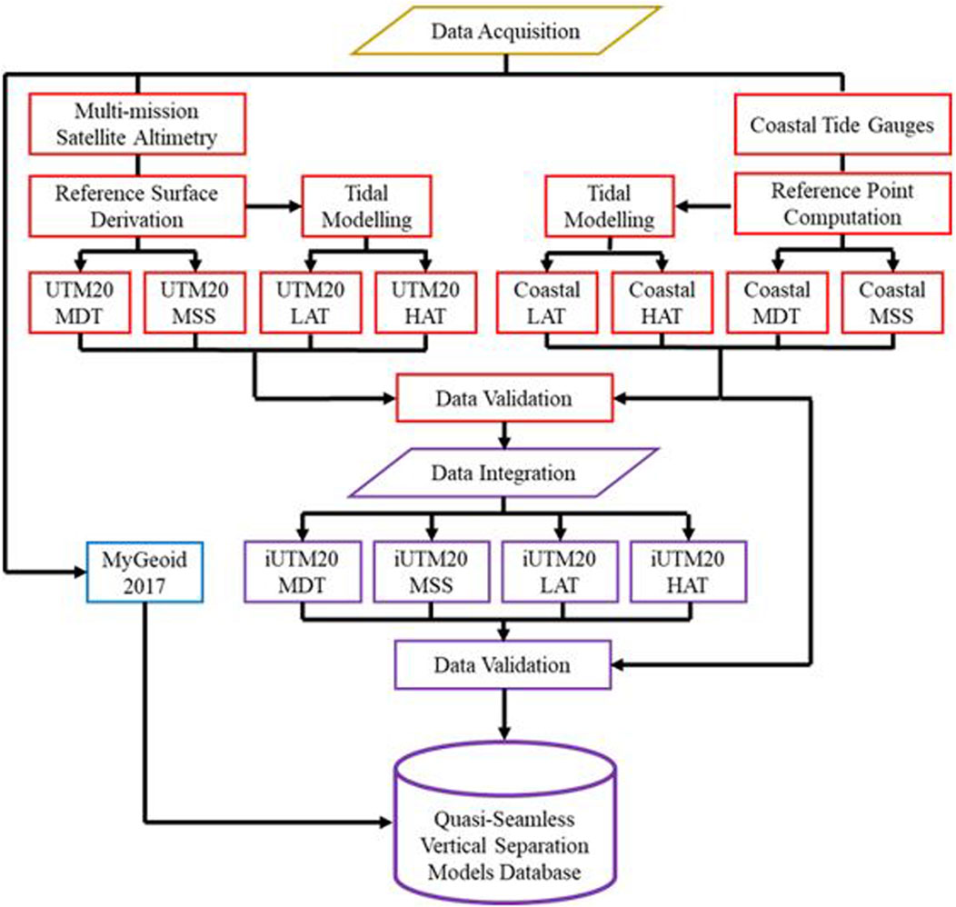
FIGURE 1. Research framework of VSEP development.

2.1.1 Satellite altimetry data

A total of ten satellite altimeter missions are used in this study, namely, TOPEX/Poseidon, Jason-1, Jason-2, Jason-3, ERS-2, Geosat Follow-On (GFO), Envisat-1, CryoSat-2, SARAL/AltiKa, and Sentinel-3A, encompassing 27 years of observation period, covering from January 1993 until December 2019. These satellite missions are essential in developing regional vertical reference surfaces, such as UTM20 MSS and MDT. Nevertheless, only TOPEX, Jason-1, and Jason-2 (denoted as the TOPEX class), and GFO mission are utilized to develop UTM20 LAT and HAT models. Satellite altimetry data are extracted and processed using the Radar Altimeter Database System (RADS). The final output of altimetry processing is along-track sea surface height (SSH). Detail descriptions of multi-mission satellite altimetry data are tabulated in Supplementary Table S2.

2.1.2 Tidal data

Tidal data from coastal tide gauges have been obtained from the DSMM through the University of Hawaii Sea Level Center (UHSLC) website. Only 11 DSMM tide gauge stations around Peninsular Malaysia are used to compute MSL, LAT, and HAT to develop the VSEP model. In addition, these 11 tide stations, including several stations in Sabah and Sarawak, are also used to validate the vertical reference surfaces derived from satellite altimetry. Supplementary Table S3 shows the list of the DSMM tide gauge stations used in this study.

2.1.3 Local geoid model

Geoid is an equipotential surface of the Earth’s gravity information, which is directly correlated with the MSL and interpreted as a surface level perpendicular to gravity. In motionless ocean without long-term atmospheric or oceanographic effects, the sea surface usually coincides with the geoid (Mills and Dodd, 2014; Yazid, 2018). However, MSL determination can differ by up to 1 m from the geoid. The geoid model devotes to the vertical component of the reference system, allowing ellipsoidal heights of the Global Positioning System (GPS) to be translated to orthometric height for practical purposes (DSMM, 2005).

The geoid is required in this study to compute MDT surfaces and as input data in the VSEP model database. Although GGM can be obtained for free through the International Center for Global Gravity Field Models (ICGEM) website, this study aims to use the local geoid model, which is Malaysian Geoid (MyGeoid). Thus, a local gravimetric geoid, namely, MyGeoid_2017, is employed in VSEP model development. This model is a newly developed continuous geoid-based vertical datum from an amalgamation of terrestrial, airborne, and satellite platforms (Jamil et al., 2017). The perk of using local geoid model is that it can express high-frequency features that are not well encapsulated by the global model without introducing an ultra-maximum spherical harmonic degree (Reguzzoni et al., 2021).

2.2 Determination of UTM20 MSS and UTM20 MDT models via satellite altimetry

The data from multi-mission satellite altimeter are extracted and processed to obtain SSH using RADS. Subsequently, the SSH data are further processed to develop MSS and MDT and to derive LAT and HAT from satellite altimetry tidal modeling. The derivation of surface-level parameters from satellite altimetry covering offshore areas is performed before assimilation with coastal tidal data. Generally, MSS has a similar definition to MSL. For example, to calculate a tidal datum, both are denoted as the arithmetic mean of hourly tidal observations over 19 years. However, MSS is a term that describes the average of satellite-derived SSH over a period of time (Andersen and Scharroo, 2011; Yuan et al., 2020). The determination of MSS is critical in various scientific research studies, particularly in the domains of oceanography, geoscience, and environmental science.

In this study, the MSS model is determined by using a temporal average method, which depends on the subsequent processes, namely, data selection and pre-processing, ERM mean track derivation from collinear analysis, removal of GM sea-level variability, crossover minimization, and data gridding. After applying the geophysical corrections and reducing the bias in the pre-processing section, the next step is to remove the sea-level variability from ERM and GM data (Hamden et al., 2021). To minimize time variation, it is necessary to handle SSH observations in the GM of satellite altimetry in a different way. Time-averaging is inappropriate for GM data due to its lack of repeating period characteristics. The approach utilized to address the seasonal signal in GM data involves the interpolation of sea-level anomalies (SLAs), as proposed by Schaeffer et al. (2012) and Jin et al. (2016). The spatial and temporal positions of the GM data are referenced using the delayed-time Developing Use of Altimetry for Climate Studies (DUACS) Level 4 gridded SLA maps (Dibarboure et al., 2012), obtained from the European Copernicus Marine Environment Monitoring Service (CMEMS) via https://resources.marine.copernicus.eu/. Hourly gridded SLA time series corresponding to the GM data are computed to make necessary adjustments. The general processing flow in establishing the UTM20 MSS model is illustrated in Figure 2.

FIGURE 2

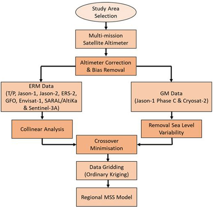
FIGURE 2. General data processing flows in MSS model computation data (Hamden et al., 2021).

MDT can be defined as the separation value spanning the geoid and MSS. Different MDT models employed different geoid models in the computation. The practical approach renders the process of quantifying MDT from MSS, and a geoid model is conceptually straightforward. A precise local gravimetric geoid, the so-called MyGeoid_2017, is selected to compute the UTM20 MDT model and represent the marine geoid model in the VSEP database. In this study, a regional UTM20 MDT is determined from the difference between the MyGeoid_2017 and regional UTM20 MSS models, as derived in Equation 1 (Hamden et al., 2021):

$\mathit{U}\mathit{T}\mathit{M}\mathbf{20}\mathit{M}\mathit{D}\mathit{T}=\mathit{U}\mathit{T}\mathit{M}\mathbf{20}\mathit{M}\mathit{S}\mathit{S}-\mathit{M}\mathit{y}\mathit{G}\mathit{e}\mathit{o}\mathit{i}\mathit{d}\_\mathbf{2017}.(1)$

The UTM20 MSS model is stated in the mean tide system, while the permanent tide system of MyGeoid_2017 is not stated. According to Keysers et al. (2013), geoid undulations can be used in any system, but EGMs are generally issued as both tide-free and zero-tide systems. Generally, regional geoids acquire their tidal system from the EGM, but the system should be specified. Therefore, it is assumed that MyGeoid_2017 is provided in a tide-free system. To precisely compute MDT, both models must be in the same permanent tide. Here, UTM20 MSS is converted to a tide-free system using the conversion formula (in cm) as expressed in Equation 2 (Ekman, 1989; Keysers et al., 2013):

${\mathit{N}}_{\mathit{n}}={\mathit{N}}_{\mathit{m}}+\left(\mathbf{1}+\mathit{k}\right)\left(\mathbf{9.9}-\mathbf{29.6}{\mathit{sin}}^{\mathbf{2}}\mathit{\varphi }\right),(2)$

where $N_n$ is the tide-free system, $N_m$ is the mean tide system, $k$ is a variable called the Love number, which depends on the mass distribution within the planet (usually taken as 0.3), and $\varphi$ is the latitude of the point. In addition, comprehensive filtering of the differences is necessary to eliminate short-scale geoid signals and to obtain a good MDT estimation. This filtering process will also eradicate the presence of residual noise in the MSS field due to unmodelled tide and the ground track striation (Farrell et al., 2012). Spatial averaging filtering methods are likely to be more decisive and precise for regional MDT applications compared with spectral filtering methods (Losch et al., 2007; Knudsen and Andersen, 2013). Spatial filters with a Gaussian-like roll-off provide more accurate results than those with sharp space cut-offs. The 2D isotropic Gaussian function is expressed as given in Equation 3 (Fisher et al., 2003; Hamden et al., 2021):

$\mathit{G}\left(\mathit{x},\mathit{y}\right)=\frac{\mathbf{1}}{\mathbf{2}\mathit{\pi }{\mathit{\sigma }}^{\mathbf{2}}}{\mathit{e}}^{-\frac{{\mathit{x}}^{\mathbf{2}}+{\mathit{y}}^{\mathbf{2}}}{\mathbf{2}{\mathit{\sigma }}^{\mathbf{2}}}},(3)$

where x is the distance from the origin in the horizontal axis, y is the distance from the origin in the vertical axis, and σ is the standard deviation of the distribution, which is also defined as the filter radius. Hence, the unfiltered regional MDT is computed by differentiating between UTM20 MSS and MyGeoid_2017, and a spatial filter is applied to smooth the MDT surfaces. The spatial filter is an average filter at which the kernel is an $nx$-by-$ny$ matrix. Variables $nx$ and $ny$ are the number of kernel points in the east–west and north–south directions, respectively. An optimal sigma (σ) should be determined to preserve true physical signal data. A higher sigma will lead to the overfiltered signal data. Nevertheless, a lower sigma will not eliminate the error from the signal data. Here, isotropic Gaussian smoothing kernel with a standard deviation (σ) of 6 is adopted to filter the noise in the 1.5-min gridded MDT. The smoothing is performed using the imgaussfilt MATLAB function. Finally, the final regional MDT (filtered) is developed by re-interpolating it into a similar grid size, as the UTM20 MSS model. The size of the study area for the UTM20 MDT model is reduced, equal to the size of MyGeoid_2017 obtained from the DSMM, which is 0^oN ≤ latitude ≤ 9^oN and 98^oE ≤ longitude ≤121^oE.

2.3 Deriving offshore tidal datum UTM20 LAT and UTM20 HAT from satellite altimetry

SSH derived from satellite altimetry is utilized in developing a regional tidal datum. Computation of LAT and HAT from satellite altimetry is carried out from only four satellite missions, namely, TOPEX, Jason-1, Jason-2, and GFO. The extracted SSH data span over 24 years for the combined TOPEX class and 9 years for the GFO mission. In theory, additional missions such as ERS-1, ERS-2, Envisat, SARAL/AltiKa, and Sentinel-3A hold the potential to contribute substantial datasets to enhance ocean tide models. However, due to their sun-synchronous sampling, the observation of solar tides, particularly the principal semidiurnal S2 constituent, is severely restricted when employing the harmonic analysis method. SSH computations are pre-processed based on the best range and geophysical correction in the Malaysian region, without applying ocean tide correction. This is to prevent the elimination of the tidal signal in SSH data. In addition, SSH induced by an ocean tide signal is the signal of interest in altimetry tidal datum modeling.

Temporal offset requires considerable attention to merge TOPEX, Jason-1, and Jason-2 time series. TOPEX was launched in September 1992 and ended in August 2002. Jason-1 then continued its mission from January 2002 until January 2009. Jason-2 was then launched in July 2008 to replace Jason-1 and ended its mission in October 2016. TOPEX SSH time series are arranged ahead of Jason-1 SSH time series and followed by Jason-2 SSH time series. The end date of TOPEX SSH data is identified, and the initial data of the Jason-1 SSH time series overlapped with the near-end TOPEX SSH data are truncated. This method is also applied between Jason-1 and Jason-2 SSH time series. It is noted that only the ERM track of TOPEX class missions are used in this study for tidal datum modeling. Meanwhile, the GFO mission is a single mission with no continuity of time series from other missions. Thus, merging the SSH time series from the GFO mission is not necessary.

In theory, a satellite altimeter that travels on the repeated orbit will coincide at the same point after completing its cycle. Nevertheless, the ground tracks practically do not accurately coincide with each other for every cycle. The orbit tracks may slide within 1–2 km for each cycle. The formation of the SSH time series is performed by extracting the SSH of each cycle at discrete points. The along-track point from the first cycle of each altimetry pass is treated as the reference for the subsequent cycles. A diameter of 7 km from each point of the reference track is plotted to identify the nearest altimetry points from the reference. SSH points from subsequent cycles within the circle of 7 km radius are selected to form time series. This is because the spatial interval of 1 Hertz (Hz) satellite altimetry footprint is approximately 7 km. Thus, the altimetry points located beyond the circle are removed as outliers.

Aliasing is an effect that distinguishes or distorts other signals when a signal reconstructed from samples is different from the original continuous signal. The TOPEX class and GFO missions suffer from tidal aliasing effects due to the long temporal sampling of the satellite altimeter (9.9156 days and 17.0505 days, respectively). The aliasing period from both missions are computed as shown in Equation 4 (Lindsley, 2013; Pirooznia et al., 2016):

${\mathit{T}}_{\mathit{a}}=\frac{\mathbf{2}\mathit{\pi }∆\mathit{s}}{\mathbf{2}\mathit{\pi }\left(\mathit{f}∆\mathit{s}-\left[\mathit{f}∆\mathit{s}+\mathbf{0.5}\right]\right)},(4)$

where $f$ is the frequency of the tidal component, $∆s$ is the period sample, and the bracket [.] in the formula of [$f∆s+0.5$] is the fix function that returns the greatest integer less than argument. The aliasing effect on the tidal signals as measured by satellite altimetry shows that each tidal constituent’s period seems to be longer than its actual period. Following that, the calculated aliasing period of each tidal constituent is utilized in harmonic analysis to derive amplitude and phase. The harmonic expression of the tidal height, $H$ at time $t$ and location $\left(\phi ,\lambda \right)$ can be expressed as shown in Equation 5 (Wijaya, 2012; Ainee, 2016; Alihan et al., 2019):

$\mathit{H}\left(\mathit{\phi },\mathit{\lambda },\mathit{t}\right)={\mathit{Z}}_{\mathbf{0}}\left(\mathit{\phi },\mathit{\lambda }\right)+{\displaystyle \sum _{\mathit{k}}}{\mathit{A}}_{\mathit{k}}\left(\mathit{\phi },\mathit{\lambda }\right)\mathit{cos}\left[{\mathit{\omega }}_{\mathit{k}}\mathit{t}-{\mathit{\theta }}_{\mathit{k}}\left(\mathit{\phi },\mathit{\lambda }\right)\right],(5)$

where $Z_0\left(\phi ,\lambda \right)$ is the MSL of analyzed data and $k$ represents the entire tidal constituents. $A_k\left(\phi ,\lambda \right)$ and ${\theta }_k\left(\phi ,\lambda \right)$ are, respectively, the tidal amplitudes and Greenwich phase lags of the tidal constituent $k$ that is estimated via the least-square method. ${\omega }_k$ represents the tidal frequency of $k$th tidal constituent. Twelve harmonic constants, namely, M2, S2, K1, O1, N2, K2, P1, Q1, MF, MM, SSA, and SA, are derived to predict the along-track tidal datums, UTM20 LAT and UTM20 HAT. To generate LAT and HAT models, the tides from both missions are predicted for a minimum duration of 19 years as proposed by Byun and Hart (2019), who acknowledge the importance of a sufficiently long tidal prediction period. Meanwhile, International Hydrographic Organization (2018) recommends using a minimum timeframe for reliable results in computing LAT and HAT.

2.4 Tide Gauge GNSS Campaign 2019

Various approaches are used to derive the connection between a vertical datum and reference ellipsoid. Typically, most Malaysian tide gauges have no information regarding the relationship between the vertical datum and ellipsoid. Conventionally, the vertical datum is referenced either to a local benchmark (BM) or the national datum. To achieve the heights of the vertical datum with respect to the ellipsoid, UTM, in collaboration with Universiti Teknologi MARA (UiTM) Arau Campus, Perlis, has implemented Tide Gauge GNSS Campaign 2019 around Peninsular Malaysia to “tie-in” the DSMM tide gauge stations with high-precision GNSS observations. This includes the GNSS observation fieldwork carried out at Pulau Pinang, Lumut, Tg. Keling, Kukup, Tg. Sedili, Pulau Tioman, Tg. Gelang, Cendering, Geting, Pulau Langkawi, and Port Klang. Supplementary Figure S1 illustrates a total of 11 DSMM tide gauge stations involved in Tide Gauge GNSS Campaign 2019. Vertical land motion (VLM) along coastal areas has emerged as a significant concern in examining a sea-level rise across multiple decades to centuries. During this extended period, a diverse array of natural- and human-induced factors can induce VLM (Wöppelmann and Marcos, 2016). The available evidence suggests that subsidence in Peninsular Malaysia was triggered by the 2004 Mw 9.2 Sumatra–Andaman earthquake. According to Simons et al. (2023), this seismic event initiated a process that resulted in gradual sinking of the land, with a recorded decrease of 3–5 cm over the past 17 years. In East Malaysia, the rates of subsidence are comparatively lower, ranging from −0.5 to −1.0 mm per year, leading to a total landfall of 2–3 cm during the same period. However, the VLM around the Malaysian coast is not considered in this study.

The tide gauge GNSS campaign was conducted from 7 to 23 February 2019, involving 11 DSMM tide gauge stations. The GNSS observations have been performed between 5 and 6 h at each station using Trimble 5700 geodetic receiver and Zephyr Geodetic antenna, as shown in Supplementary Figure S2. Trimble Business Centre Version 5.0 (TBC v5.0) has been used to process the GNSS observations data with the cutoff angle and data interval set at 13° and 10 s, respectively. The relative positioning technique is used to resolve the GNSS data where at least 3 to 4 MyRTKnet stations have been adopted as reference stations. Due to poor sky view and multipath issues, six out of 11 tide gauges are unsuitable for direct GNSS observations on the tide gauge benchmark (TGBM). Thus, a new GNSS point, denoted as temporary benchmark (TBM), is established near the TGBM with a good sky view clearance, as shown in Supplementary Figure S2A. After GNSS observation, a precise levelling survey has been conducted using Trimble DiNi to transfer the ellipsoidal height from the new GNSS point to the TGBM. Here, the height difference obtained from precise levelling is applied to the ellipsoidal height of new GNSS point to obtain TGBM point relative to ellipsoid. Supplementary Table S4 lists the height difference of precise levelling from the new GNSS point to the six TGBMs involved.

2.5 Determination of UTM20 MSS and UTM20 MDT at coastal tide gauges

The ellipsoidal height of MSL is determined from GNSS observations at TGBM. These data are processed in the International Terrestrial Reference Frame 2014 (ITRF2014). To achieve this, all MyRTKnet stations involved have been realized into ITRF2014 using Bernese GNSS Software Version 5.2. Then, the final coordinates of MyRTKnet stations in ITRF2014 are adopted for TBC processing to compute the GNSS solutions at TGBM. The MSL at tide gauges is derived from an observation period of 23 years from 1993 to 2015 using a simple averaging method. Here, the local MSL is relative to the zero-tide gauge. Thus, the local MSL must be transformed into MSL relative to the reference ellipsoid. Supplementary Figure S3 illustrates the relationship of various vertical surfaces to achieve tidal measurement with respect to the ellipsoidal surface (Hamden et al., 2021). The formula to obtain MSL with respect to the Geodetic Reference System 1980 (GRS80) ellipsoid is shown in Equation 6:

${\mathit{h}}_{\mathit{M}\mathit{S}\mathit{L}}={\mathit{h}}_{\mathit{G}\mathit{N}\mathit{S}\mathit{S}}-∆{\mathit{H}}_{\mathit{L}\mathit{E}\mathit{V}}+∆{\mathit{H}}_{\mathit{M}\mathit{S}\mathit{L}},(6)$

where $h_{MSL}$ is the MSL height above the reference ellipsoid, $h_{GNSS}$ is the ellipsoidal height from GNSS observation, $∆H_{LEV}$ indicates the TGBM height above zero-tide gauge, and $∆H_{MSL}$ is the MSL height above zero-tide gauge. In determining the MDT or sea surface topography (SST), the geoid height value must be in the same reference ellipsoid and same permanent tide system with the MSL ellipsoid at tide gauges. The ellipsoid of MSL is given in a tide-free system. This has been stated by Keysers et al. (2013) where the ITRF and its realizations including the GNSS ellipsoidal height system employ the tide-free system. Apart from that, MyGeoid_2017 is given in a tide-free system and interpolated to the tide gauge locations using the bilinear interpolation method. Therefore, the ellipsoid of MSL height can be directly subtracted with MyGeoid_2017 to obtain geodetic MDT at tide gauges.

2.6 UTM20 LAT and UTM HAT tidal datum computations at coastal tide gauges

A tide gauge is a fixed point of the reference surface to observe the water level and is set up with a tide staff or other reference to continuously estimate the time series of the sea level. It has a long and high-frequency water level record (hourly data) which is beneficial for ocean investigation, including tidal analysis, prediction, and climate change. The hourly tidal data obtained via the UHSLC website (https://uhslc.soest.hawaii.edu/) are filtered using the statistical control quality method. This method implements the multiple sigma control limit, in which the multiple gross errors can be identified (Elgazooli and Ibrahim, 2012; Alihan, 2018). The sea-level time series from tide gauges are filtered using three-sigma (σ) control limits. When all measurement points are within 3σ control limits, the time series is statistically controlled, indicating that there is no gross error in the data. Consequently, the tidal data beyond the limit are excluded using the moving average technique. Then, the filtered tidal data are used to perform the tidal harmonic analysis where a tidal time series is treated as the composition of several cosine waves to estimate the presence of the tidal signal. The harmonic analysis coefficient parameters are used to estimate the amplitude and phase of principal tidal constituents.

A total of 68 tidal constituents have been estimated at each tide gauge, and these tidal constituents are subsequently used to predict the tides. The tides are predicted from 1993 to 2019, spanning more than 19 years. This is to complete the precession cycle of the moon nodes, where it takes 18.61 years to go completely around and back to their original position. Hence, LAT and HAT at tide gauges are generated from the lowest and highest predicted tides, respectively. Supplementary Figure S4 illustrates the tidal analysis and prediction, including the residuals (Top) and the 19-year tidal prediction (bottom) to determine the LAT and HAT.

2.7 Integration of vertical datum between coastal and offshore

A continuous vertical datum is created by combining the coastal and offshore datasets. The coastal datasets referred to the vertical reference point computed from the DSMM coastal tide gauges, while the offshore datasets referred to the vertical reference surfaces derived from satellite altimetry. MSS, MDT, LAT, and HAT are the vertical datums involved in developing the continuous VSEP model in the Malaysian region. It is noted that the integration of the vertical datum has only been conducted around the Peninsular Malaysia region, and Sabah and Sarawak are excluded due to the limitation of coastal datasets.

2.7.1 Establishment of integrated UTM20 MDT and MSS models

Satellite altimetry-derived MSS is the dominant component in the open sea, but its quality deteriorates near the coast. An integrated UTM20 MSS (iUTM20 MSS) has been developed by combining the tide gauge data to enhance the satellite altimetry-derived UTM20 MSS in the coastal zone. Before integration, both coastal and offshore data must be referenced to a common datum, epoch, and similar permanent tide system. The common datum selected for the iUTM20 MSS is WGS84 (G1762), as most of the hydrographic practices use it as a working datum. The epoch selected is from 1993 to 2019, and a tide-free system is considered for this integration.

Table 1 shows the parameters of tide gauges and satellite altimetry MSS before integration. The integration is still being conducted despite the datum difference between coastal tide gauges and satellite altimetry. According to Quality Positioning Services (2020), ITRF2014 and WGS84 (G1762) are likely to coincide with minimal discrepancy at the centimeter level, yielding conventional zero transformation parameters. Generally, the developed UTM20 MSS is available in the mean tide system and relative to the T/P ellipsoid. Thus, the UTM20 MSS tide system and ellipsoid require conversion to the common parameters chosen. For the tide system, Equation 2 is used for conversion into a tide-free system. Meanwhile, transformation into the WGS84 ellipsoid is performed by applying an offset of −71 cm. This offset is based on Terry (2004), where many applications assume that T/P elevations are 71 cm higher than WGS84 elevations for north or south latitudes of ±40 degrees.

TABLE 1

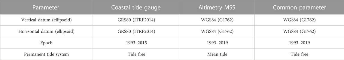
TABLE 1. Parameters used before integration.

There are few elements required for the development of iUTM20 MSS, including coastal tide gauge-derived ellipsoid-based MSS extended to 10 km offshore, the satellite altimetry-derived UTM20 MSS extended from 20 km offshore to the open sea, and interpolation across the caution zone (10–20 km) between tide gauge-derived MSS and UTM20 MSS. Deng et al. (2002) recommended that altimetry data must be used with caution for distance less than 20 km from the coastline. In other international projects, such as AusCoastVDT, only 4-km tide gauge data and 22-km purely satellite altimetry data are used. Meanwhile, VORF uses only 14 km of the coast tide gauge data and uses purely satellite altimetry data beyond 30 km of the coastline. In this research, the tide gauges are first interpolated into a surface extending from the coastline to 10 km offshore to ensure that the satellite altimetry data have no impact within its zone of exclusion. Malaysia has a sparse distribution of tide gauges, and these data make it impossible to conduct meaningful statistical analysis of the ellipsoidal MSL or MDT around the coast. Therefore, the interpolation methods are adopted to simplify the proof of concept. Three interpolation methods have been investigated to extend the Malaysian tide gauge data to 10 km offshore: inverse distance weighting (IDW), ordinary kriging, and spline.

ArcGIS software is used to create a coastal grid of MSS and MDT. Figures 3A–D illustrate the process to create the coastal grid for MSS and MDT models. First, 11 tide gauge-derived MDT values are imported into the database layer, as shown in Figure 3A. The extended 10-km offshore area is created using the buffer zone function, as shown in Figure 3B. Then, the 1.5-min spatial grid is overlaid within the buffer zone area. The grid points, which outside the buffer zone, are truncated to form a coastal grid, as shown in Figure 3C. MDT values at each tide gauge are interpolated into the coastal grids within the 10-km buffer zone.

FIGURE 3

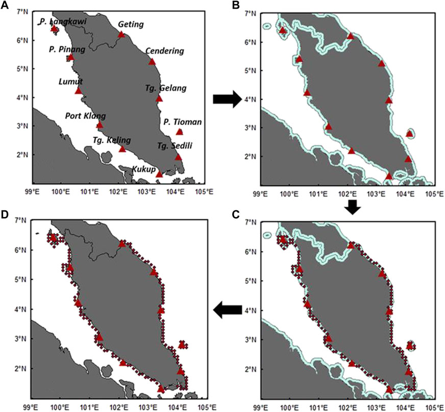
FIGURE 3. (A) Eleven tide gauges imported into ArcGIS. (B) Creating a buffer zone of 10 km extended to the offshore. (C) Truncating the grid points beyond the buffer zone. (D) Final coastal grid points for MSS and MDT models.

Satellite altimetry is supplied from UTM20 MSS, which is the regional MSS model developed by UTM. Iliffe et al. (2013) mentioned that any data within 14 km of the coast were regarded as unreliable due to potential contamination of the altimetric footprint by land and were rejected from the dataset for the case of the VORF project. However, altimetry data proximity to the coast within Malaysian seas had been investigated by Hamden et al. (2019). The altimetry data beyond 10–20 km are reliable for assessing the sea level, as shown in Figure 3. The standard deviation of range for each satellite mission increases drastically as they approach the coastal zone. The degradation of the altimetry quality data is due to the contamination within the radar footprint toward the land. Each satellite mission has its standard deviation of range due to its radial orbit accuracy. For this study, it is decided to use purely satellite altimetry outside 20 km buffer from the coastline. After computing the interpolated MDT points within the caution zone, this dataset is combined with the tide gauge at 0–10 km surface and altimetry data beyond 20 km offshore by reinterpolating onto a 1.5-min grid using the ordinary kriging technique. The final integrated MDT (iUTM20 MDT) is the surface resulting from the kriging interpolation. Subsequently, the integrated UTM20 MSS is obtained by the summation of iUTM20 MDT with MyGeoid_2017, as shown in Supplementary Figure S5.

2.7.2 Establishment of integrated tidal datums, iUTM20 LAT and HAT

The available data sources for integration of tidal datums are discrete measurements of tidal levels at coastal tide gauges and satellite altimetry-derived regional ocean tide models. The coastal tide gauges are retrieved from the DSMM, which cover only 11 points in Peninsular Malaysia. These tide gauges possess observation record spanning over 19 years, providing ample data to directly predict LAT and HAT. To expand the coverage of coastal tide gauges, the inclusion of NHC tide tables is considered. However, it is unfit as the observation durations and epochs in the NHC tide tables exhibit significant variations, with the majority of them having observation periods of less than 19 years. Nevertheless, a level known as CD is available at all tide gauges provided in the DSMM tide observation record book. CD is approximated to the LAT value by scaling the available lowest level from the shorter time series, while LAT is determined from the long-term data observation. The LAT and HAT values at tide gauge stations are derived as expressed in Equations 7, 8, respectively.

${\mathit{L}\mathit{A}\mathit{T}}_{\mathit{M}\mathit{S}\mathit{L}}={-\mathit{Z}}_{\mathbf{0}}-{\mathit{L}\mathit{A}\mathit{T}}_{\mathbf{0}},(7)$

${\mathit{H}\mathit{A}\mathit{T}}_{\mathit{M}\mathit{S}\mathit{L}}={\mathit{H}\mathit{A}\mathit{T}}_{\mathbf{0}}-{\mathit{Z}}_{\mathbf{0}},(8)$

where ${LAT}_{MSL}$ is the height of LAT with respect to MSL, $Z_0$ is the observation of MSL above the zero-tide gauge, and ${LAT}_0$ is the height of LAT above the zero-tide gauge. Meanwhile, ${HAT}_{MSL}$ is the height of HAT with respect to MSL, and ${HAT}_0$ is the height of HAT above the zero-tide gauge. Supplementary Table S5 shows the LAT and HAT values derived from the aforementioned equation. These values are integrated with the satellite altimetry-derived LAT and HAT models. In practice, CD values are obtained from the DSMM tide observation record book, while LATs are obtained through tidal modelling. Both CD and LAT are relative to the zero-tide gauge, and the RMS difference can be computed as shown in Table 2. The value of the RMS difference is minimal, which is 0.058 m; thus, it is assumed that CD is equal to LAT in this study.

TABLE 2

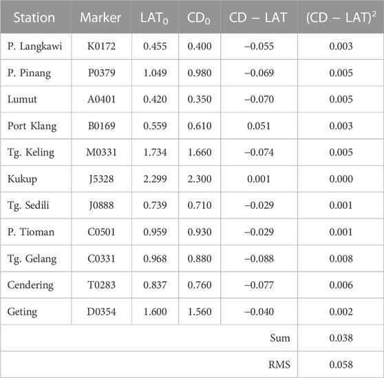
TABLE 2. RMS differences between CD and LAT at tide gauges [units are in meters].

Satellite altimetry-derived tidal models (UTM20 LAT and HAT) are used to cover the offshore regions. However, the degradation of the altimetric models is expected when close to land. Therefore, the gridded altimetric-derived tidal models are truncated within 20 km from the coastal to minimize errors near coastal. Figures 4A, B show the distribution of the computed tidal datums at the 11 tide gauge stations and the truncation of 20 km from coastal of gridded regional tidal models, respectively. These two data sources are merged and interpolated using the thin-plate spline (TPSL) method to develop integrated tidal datums, as shown in Figure 4C. Finally, the integrated tidal datums are then re-interpolated to a 1.5-min spatial resolution grid adopting the grid size of iUTM20 MSS and MDT models.

FIGURE 4

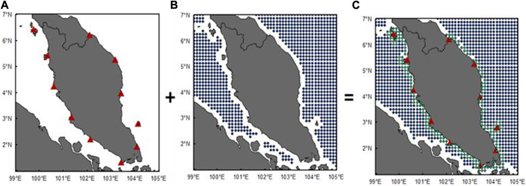
FIGURE 4. (A) Distribution of computed tidal datums at the 11 tide gauges. (B) Grid points of satellite altimetry-derived tidal datums (UTM20 LAT and HAT). (C) Combination of coastal and offshore tidal datums using the TPSL interpolation method.

2.8 Statistical data assessment

2.8.1 Assessment of altimetry tidal analysis and prediction

The quality assessment of the satellite-derived tidal constituents (SDTC) is crucial before conducting any further analyses, such as tidal range computation and tide prediction. The SDTC obtained from harmonic analysis are assessed by comparing with selected DSMM tide gauge stations at the coastal region. The closest altimetry footprint to the tide gauge locations is compared with tidal constituents derived from tide gauges, and eight tidal constituents (M2, S2, K1, O1, P1, Q1, N2, and K2) are used for assessment in this study. The discrepancy between the amplitudes and phases of derived harmonic constants and other data sources, including tidal gauges and tide models, are quantified using root mean square misfit (RMS_misfit) as expressed in Equation 9:

${\mathit{R}\mathit{M}\mathit{S}}_{\mathit{m}\mathit{i}\mathit{s}\mathit{f}\mathit{i}\mathit{t}}={\left\{\frac{\mathbf{1}}{\mathbf{2}\mathit{N}}{\displaystyle \sum _{\mathit{k}=\mathbf{1}}^{\mathit{N}}}\left[{\left({\mathit{A}}_{\mathit{o}}\mathbf{cos}{\mathit{G}}_{\mathit{o}}-{\mathit{A}}_{\mathit{m}}\mathbf{cos}{\mathit{G}}_{\mathit{m}}\right)}^{\mathbf{2}}+{\left({\mathit{A}}_{\mathit{o}}\mathbf{sin}{\mathit{G}}_{\mathit{o}}-{\mathit{A}}_{\mathit{m}}\mathbf{sin}{\mathit{G}}_{\mathit{m}}\right)}^{\mathbf{2}}\right]\right\}}^{\frac{\mathbf{1}}{\mathbf{2}}},(9)$

where $N$ is the number of assessment points utilized and $A_o$ and $G_o$ are the amplitude and phase estimated from satellite altimetry data, respectively. Equivalently, $A_m$ and $G_m$ are, respectively, the amplitude and phase produced by other sources, in this case, tide gauges and DTU10 ocean tide model. After RMS computation, root sum square (RSS) is calculated for the overall tide models generated from this study. The formula of RSS is described in Equation 10:

$\mathit{R}\mathit{S}\mathit{S}={\left({\displaystyle \sum _{\mathit{l}=\mathbf{1}}^{\mathit{M}}}{\mathit{R}\mathit{M}\mathit{S}}_{\mathit{l}}^{\mathbf{2}}\right)}^{\frac{\mathbf{1}}{\mathbf{2}}},(10)$

where $M$ represents the total tidal constituents used in this study and ($RMS$_l²)^1/2 is the square of root mean square for each tidal constituent. Apart from that, two root mean square error (RMSE) calculations as shown in Equation 11 are also performed in this study. First, the RMSE is calculated to determine the reliability of the anticipated SSH derived from satellite altimetry by comparing the predicted SSH with the observed SSH. The second assessment determines the best interpolation tidal datum surfaces in the studied region by calculating the RMSE values between the interpolated points from two techniques and the selected coastal tide gauges.

$\mathit{R}\mathit{M}\mathit{S}\mathit{E}=\sqrt{\frac{\sum {\left({\mathit{x}}_{\mathit{o}}-{\mathit{x}}_{\mathit{t}}\right)}^{\mathbf{2}}}{\mathit{n}},}(11)$

where $x_o$ is the value of predicted SSH and interpolated value, $x_t$ is the true value, which refers to the observed SSH or selected coastal tide gauges, and $n$ is the total number of samples.

2.8.2 Validation of integrated VSEP models

Validation of the developed VSEP surfaces can be performed in the coastal area by installing a tide gauge, in which the ellipsoidal height is established through GNSS observation. Meanwhile, validation in the offshore can be performed by deploying GNSS buoy and establishing the CD relative to the ellipsoid through tidal transfer from existing shore gauges. However, some limitations have been encountered during the validation of VSEP models in this study. One of them is the difficulties in obtaining offshore tide gauges in Malaysian regions, although a request letter of data collection for this research had been submitted to the related offshore authorities. In addition, the long-term tidal data near coastal are very limited, and most of the data have been used in the integration process. Hence, the DSMM tide gauge stations are utilized to validate the continuous VSEP surfaces in the coastal region. This is purely a measure of precision as all possible data have been utilized for the surface computation.

3 Results and discussion

3.1 Assessment of derived tidal constituents from satellite altimetry with tidal data

In this study, tidal datums derived from satellite altimetry focus only on LAT and HAT. Satellite-derived SSH time series from 24 years of TOPEX ERM mission and 9 years of GFO mission are analyzed using the harmonic approach to estimate 12 selected tidal constituents (M2, S2, N2, K2, K1, O1, P1, Q1, MF, MM, SSA, and SA). Supplementary Figure S6 shows the along-track amplitudes of the 12 major tidal constituents. Apparently, four tidal constituents (M2, S2, K1, and O1) show the most dominant tidal characteristic within the study area and have recorded higher amplitude values than the other eight constituents. These four tidal constituents are the most primary components that explain a simple model of the Earth–Sun–Moon system. The fundamental forces compelling the ocean tide signal are due to the gravitational effect induced by the moon and the sun (Lindsley, 2013).

Tidal data from seven selected tide gauges are utilized to validate the accuracy of the derived tidal constituents from satellite altimetry. The selected tide gauges include Tg. Sedili, P. Tioman, Tg. Gelang, Geting, Bintulu, Miri, and Kota Kinabalu. These tide gauges are selected based on the nearest approximation between satellite altimetry tracks and the tide gauges. In addition, the comparison between the nearest grids of DTU10 global tide models and the seven tide gauges is also conducted to determine whether the best accuracy of tidal constituents is obtained from the SDTC model or DTU10 global ocean tide model or otherwise. The development of the DTU ocean tide model is based on the finite element solution (FES 2004) and the adoption of the response method technique established by Munk and Cartwright (1966). This model uses 17 years of sea-level data from multi-mission satellite altimetry from September 1992 to December 2009. Although this study uses a similar platform as DTU10, which is satellite altimeter, it differs in terms of tidal analysis method and temporal altimetry data. This study also involves the GFO mission to derive tidal constituents. The DTU10 ocean tide model is obtained from the FTP DTU website (https://ftp.space.dtu.dk/pub/DTU10).

The nearest along-track points of SDTC to the tide gauge stations are identified and extracted. The locations and distances between tide gauge stations and the nearest point of the altimetry track are tabulated in Supplementary Table S6. In this study, two tracks of GFO altimetry and five tracks of TOPEX class are involved in the validation process. The nearest distance is at the Miri tide gauge, which is 9.14 km, and the longest distance between both points is located at the Bintulu tide gauge, which is 66.61 km. It has perceived that the maximum range between the two points is closer than that in the previous studies by Daher et al. (2015) and Fu et al. (2020), where the maximum ranges from both studies are 124 km and 77 km, respectively. The RSS values of eight tidal constituents between two models (SDTC and DTU10) and each tide gauge station are computed and presented in Figure 5. The figure depicts that SDTC provide promising RSS results compared to DTU10 in all tide gauges involved. There are significant differences in RSS values between SDTC and DTU10 located at Tg. Sedili, Geting, and Bintulu tide gauges. The differences might be due to the interpolation error of the DTU10 grid model to the tide gauge station and the insufficient time span of altimetry time series in estimating tidal constituents.

FIGURE 5

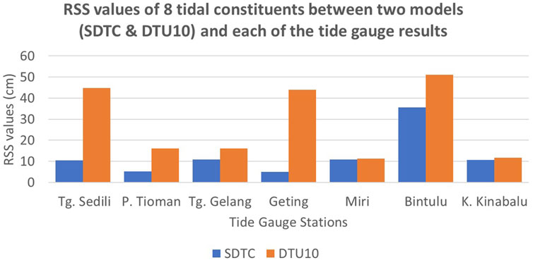
FIGURE 5. RSS values of eight tidal constituents between two models and each tide gauge.

Based on the previous study by Fu et al. (2020), the RSS values for along-track satellite altimetry points were set less than 8 cm in the deep ocean (depth >200 m). Thus, this study follows the criterion of 8 cm to determine whether the SDTC are well estimated or not. Two out of seven tide gauge stations, which are P. Tioman and Geting, have passed the criterion and have high-precision outcomes with RSS values of 5.3 cm and 5.0 cm, respectively. The Bintulu station has the highest RSS value, which is 35.5 cm. This is expected due to the longest distance between the altimetry point and the tide gauge stations. Other stations have recorded the RSS values within 10 cm. The outcomes are considered good even though the RSS values do not achieve the 8 cm criterion. For instance, the nearest SDTC to the Tg. Sedili and Tg. Gelang are from the GFO mission, where the time series data for tidal constituent estimation are limited. In addition, the depth in the study area is mainly less than 200 m. Therefore, it is expected that the RSS values could exceed 8 cm. It can be inferred that high precision of satellite-derived tidal constituents has been achieved with the TOPEX class satellite mission. This is because the satellite altimetry time series from TOPEX class spans over 24 years where all the constituents have met the criterion for the 19-year time series, and all tidal constituents can be appropriately estimated. Therefore, the precision of tidal constituents estimated from satellite altimetry data is relatively acceptable in most shallow water locations.

3.2 Assessment of altimetry tidal prediction and residuals

Tides in this study are predicted based on the estimated tidal constituents. Supplementary Figure S7 illustrates the predicted time series at each along-track altimetry point. The study area in this figure is reduced to follow the size of the study area from the UTM20 MDT model. This is because each VSEP model produced must be in the same size as the study area before it is archived in the database. The black triangles in Supplementary Figure S7 indicate the coastal DSMM tide gauge stations used to assess the estimated offshore tidal datum. Each point from the along-track predicted SSH time series has been randomly selected (labelled as red dots in Supplementary Figure S7) at each of the Malaysian seas. The selection is made to visualize the modelled time series. It is noted that the point must be selected in the offshore area.

Supplementary Figures S8A–D show the time series of selected modelled SSH and its residuals from the TOPEX class on the left column and the GFO mission on the right column. The observed and predicted SSH time series are plotted in blue and green lines, respectively. These residuals are derived by computing the differences between the predicted and observed SSH time series. Subsequently, the quality of the predicted SSH can be determined based on these residuals using RMSE computation. Apparently, the SSH time series data from the TOPEX class are denser than the GFO mission. This is because the repeat period of the TOPEX class is shorter, which is 9.9156 days, compared to GFO, which is 17.0505 days. The highest RMSE value between observed and predicted SSH from TOPEX is recorded at Malacca Strait, followed by the Celebes Sea, the Sulu Sea, and the South China Sea, which is 10.1 cm, 9.8 cm, 7.6 cm, and 7.3 cm, respectively. This might be because Malacca Strait is a closed sea with tidal characteristics that is likely to have a large gradient. Nevertheless, the highest RMSE value from the GFO mission is recorded at the Celebes Sea, followed by Malacca Strait, the Sulu Sea, and the South China Sea, with values 10.9 cm, 7.9 cm, 7.0 cm, and 6.5 cm, respectively. Therefore, it can be inferred that the precision of tidal prediction from both missions are reasonable at the offshore area since the RMSE values are within the range 6.5–10.9 cm.

3.3 Statistical assessment of satellite altimetry-derived UTM20 LAT and HAT

LAT is defined as the lowest water level, which can be predicted to occur under average meteorological conditions. Meanwhile, HAT is defined as the highest water level, which normally occurs when any astronomical conditions are combined. Both tidal datums can be derived by analyzing several years of tidal data or tidal predictions, usually 18.6 years to account for a complete nodal cycle. In this study, the SSH time series from the TOPEX class and GFO missions are predicted for at least 19 years or more. The predicted time series from the TOPEX class is from 1993 until 2019, while from GFO, it is from 2000 until 2009. The lowest and highest time series of predicted tides indicate the LAT and HAT, respectively. Subsequently, the derived LAT and HAT from the along-track satellite altimetry are interpolated and validated against the selected coastal DSMM tide gauges as distributed in Supplementary Figure S7. The derived tidal datums are converted relative to MSL prior to the results to allow comparison with the tide gauges.

The combination of TOPEX class and GFO along-track missions (LAT_MSL and HAT_MSL) is interpolated into a regular grid of 0.125° using ordinary kriging and minimum curvature spline methods, as shown in Supplementary Figure S9. This figure clearly indicates that the middle part of the Malacca Strait has the greatest tidal range of LAT_MSL and HAT_MSL compared to other regions, with values up to −2.6 m and 3.0 m, respectively. The tidal range of LAT_MSL and HAT_MSL in the middle of the South China Sea, Sulu Sea, and Celebes Sea depicts the values within −0.9 m to −1.1 m for LAT_MSL and within 0.9–1.2 m for HAT_MSL. The greatest tidal range of LAT_MSL and HAT_MSL can also be observed at the southwest of East Malaysia in the South China Sea, with values up to −2.1 m and 2.2 m, proportionately. Meanwhile, near the Gulf of Thailand, the northwestern part of the South China Sea depicts the lowest tidal range of LAT_MSL and HAT_MSL, with values near zero meters. Apparently, the tidal ranges mainly are larger near the coastal areas than the offshore areas. It is visible at the coastal part of the Celebes Sea, as shown in Supplementary Figure S9. The reason is that the satellite altimetry data acquired near the coastlines are contaminated by the inclusion of land in the footprint signal or the fact that the tide is on the ebb (Fok, 2012). Moreover, the tidal datum models interpolated using the ordinary kriging method generate smoother contour lines than the models interpolated using the minimum curvature spline method. These gridded offshore tidal datum models are then validated with the selected coastal tide gauges to determine the best interpolation method.

Generally, the optimal method to validate satellite altimetry-derived LAT and HAT is demonstrated by comparing them with the offshore tide gauges. However, the lack of establishment of offshore tide gauges and the difficulty in obtaining offshore tidal data from offshore authorities hinder this validation method. Thus, this paper adopts the statistical assessment by validating the UTM20 LAT and HAT models with 10 selected DSMM tide gauges, as shown in Supplementary Figure S7. The assessment results of LAT_MSL and HAT_MSL are described in Supplementary Table S7 and Supplementary Table S8, respectively. For UTM20 LAT, the RMSE values obtained between the minimum curvature spline model and in situ data are lower than those of the ordinary kriging model, which recorded 25.5 cm and 31.8 cm, respectively. Meanwhile, the RMSE values of UTM20 HAT between minimum curvature spline and in situ data are also lower than those of the ordinary kriging model, which yield 17.4 cm and 33.8 cm, respectively. Thus, it can be inferred that the offshore tidal datum models generated using the minimum curvature spline method have better agreement with coastal tide gauges compared to ordinary kriging models, despite the ordinary kriging producing smooth contour surfaces.

3.4 Analysis of the vertical datum at coastal tide gauges

Four types of vertical datums computed at coastal tide gauges are MSL, MDT, LAT, and HAT. These datums are then integrated with the vertical reference surfaces derived from satellite altimetry data. Only 11 coastal tide gauges along Peninsular Malaysia are used to compute the vertical datum in this research, since Tide Gauge GNSS Campaign 2019 could only cover the areas around Peninsular Malaysia. MSL values are obtained at each tide gauge by conventionally averaging the hourly tidal data. It is noted that the averaged values are relative to the zero-tide gauge. Thus, these values must be shifted to the reference ellipsoid by applying Equation 6. Subsequently, MDT values are computed by subtracting the derived MSL values with the interpolated MyGeoid_2017 at tide gauge stations. The bilinear interpolation method is adopted to interpolate the MyGeoid_2017 to the tide gauge stations.

Supplementary Table S9 tabulates the GNSS processing results of Tide Gauge GNSS Campaign 2019 using TBC v5.0. The stations marked as TBM1 until TBM6 indicate that the GNSS observation are not directly conducted on the TGBM due to poor sky-view conditions and might be induced by multipath signals. Instead, the GNSS observations are conducted on the temporarily established points to obtain ellipsoidal height. Then, the final ellipsoidal height is transferred to the TGBM through precise levelling, as described in Section 2.4. The findings show that the ellipsoidal height at P. Langkawi, P. Pinang, Lumut, and Geting are located below the ellipsoidal surface and thus the negative values. Good accuracies are displayed on the latitude and longitude of GNSS results, where the standard deviation is recorded less than 1 cm. Furthermore, the standard deviation of ellipsoidal height ranges from 0.7 cm to 4.8 cm.

Table 3 shows the computation of MSL and MDT at 11 DSMM coastal tide gauges. The MSL values relative to zero-tide gauge (hereinafter ∆H_MSL) are computed for 23 years from 1993 to 2015. It is found that the MSL values vary at each location, which range from 2.233 m to 4.030 m along Peninsular Malaysia. Here, the separation offset between the computed MSL and MyGeoid_2017 is computed to obtain MDT values, as shown in Supplementary Figure S10. The results show that P. Tioman displays the largest separation offset between MSL and MyGeoid_2017, which recorded 1.053 m, while P. Langkawi records the lowest separation offset with 0.651 m. It also can be inferred that the slope of MDT values increases from north to the south of Peninsular Malaysia at both west and east coast areas. In general, along the west coast, the separation offset between UTM20 MSS and the MyGeoid_2017 model shows a progressive latitude-dependent trend consistent with the findings from Mohamed (2003) and Pa’suya (2020). The computation of MDT at coastal tide gauges is very significant in this research as it can facilitate the integration between the vertical reference surface at coastal and offshore areas to obtain a smooth continuous model of MSS. This MSS model is established by recombining the integrated MDT with the local gravimetric geoid model, MyGeoid_2017.

TABLE 3

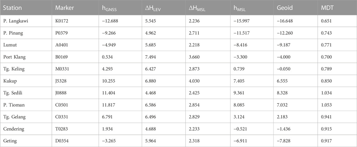
TABLE 3. Computation of MSL and MDT at coastal tide gauges [units are in meters].

For the computation of LAT and HAT, the filtered hourly tidal data are analyzed and predicted using the harmonic analysis approach. The computed LAT and HAT values at each tide gauge, including the RMSE of residuals, are tabulated in Supplementary Table S10. The RMSE of residuals is the accuracy of the predicted sea level, which is calculated between the predicted and observed sea levels using Equation 11. The results show that the accuracy of the predicted sea level at each tide gauge is between 9.5 cm and 13.8 cm, where Tg. Keling records the highest accuracy and Port Klang displays the lowest accuracy. The computation of LAT and HAT relative to the reference ellipsoid is based on the modification of Equation 3.9, in which the parameter of ∆H_MSL is replaced by ∆H_LAT and ∆H_HAT. Here, the findings show that the LAT values from tide gauges are within the range −17.778 m–7.675 m. Meanwhile, the HAT values are within the range −14.246 m–10.788 m.

3.5 Analysis of integrated UTM20 MDT and MSS

The establishment of UTM20 MSS, MDT, LAT, and HAT is successfully conducted to represent the offshore datasets of the vertical datum. In addition, these four vertical datums are also well developed at each tide gauge station involved in this research to represent the coastal datasets. A continuous VSEP model is developed by combining offshore and coastal surfaces. The ellipsoid-based transformation approach utilizes a set of gridded surfaces, in which each surface defines the separation of one vertical datum from the WGS84 ellipsoid. The four gridded vertical separation surfaces are MSL-WGS84, MyGeoid_2017-WGS84, LAT-WGS84, and HAT-WGS84.

The tide gauge-derived MDT is interpolated to a surface extending from the coastline to 10 km offshore. Three interpolation techniques, namely, IDW, ordinary kriging, and thin-plate spline, have been adopted to determine the optimal interpolation for coastal datasets. Table 4 shows the statistical differences between the actual and predicted values of tide gauge MDT using three interpolation techniques. The spline technique displays the optimal accuracy of MDT surfaces, followed by IDW and Ordinary Kriging, which recorded 0.2 cm, 0.48 cm, and 0.52 cm, respectively. Evidently, all interpolation techniques yield better than 1 cm accuracy when compared to the input tidal data.

TABLE 4

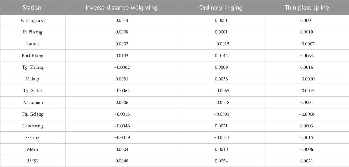
TABLE 4. Statistical results of differences between actual and predicted tide gauge-derived MDT using three interpolation techniques [units are in meters].

For further investigations on each interpolation method, one tide gauge at a time is removed, and the MDT surface is then re-interpolated. The actual value for the removed tide gauge is compared to its predicted values. Supplementary Table S11 shows the statistical results of the differences between the actual and predicted values using the removal test for tide gauge-derived MDT from three interpolation techniques. The findings show that the IDW and ordinary kriging techniques are rejected based on their higher mean than the spline method. The standard deviation of the spline method is substantially better than the standard deviation of IDW and ordinary kriging. Apart from that, spline also generates the smoothest surface and fits well with satellite altimetry data, as shown in Figure 6. Therefore, the spline technique is well suited to create gradually changing surfaces, such as elevation and sea-level heights. The UKHO also uses it to represent LAT relative to MSL (Turner et al., 2010).

FIGURE 6

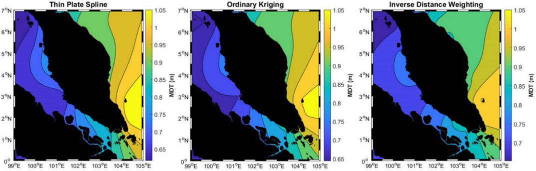
FIGURE 6. Pattern of MDT surfaces using three different interpolation techniques.

Here, the interpolation techniques disregard islands or any form of shorelines; instead, the data are interpolated assuming all surfaces are ocean. Incorporating a technique that determines the correlation of tidal data by distance over sea and utilizing a coastline polygon to account for islands’ impacts and bending shorelines may lead to future advancements in this research. Enhancement by adopting the suggested approach would be ideal with the expansion of tide gauge distribution to describe MSL variation along the coast better. Furthermore, establishing a coastal thread or hydrodynamic stream, as recommended by Keysers et al. (2013), could be adopted for future improvements. After creating the MDT surfaces extending 10 km from the coastline, these coastal datasets are integrated with 20 km offshore of UTM20 MDT by adopting ordinary kriging and minimum curvature spline methods. The statistical results of the difference between in situ and two interpolation MDT models are shown in Table 5. The findings present that the minimum curvature technique records slightly better accuracy than ordinary kriging with the standard deviation values of 1.8 cm and 1.9 cm, respectively. Both interpolation models yield the mean difference below 1 cm.

TABLE 5

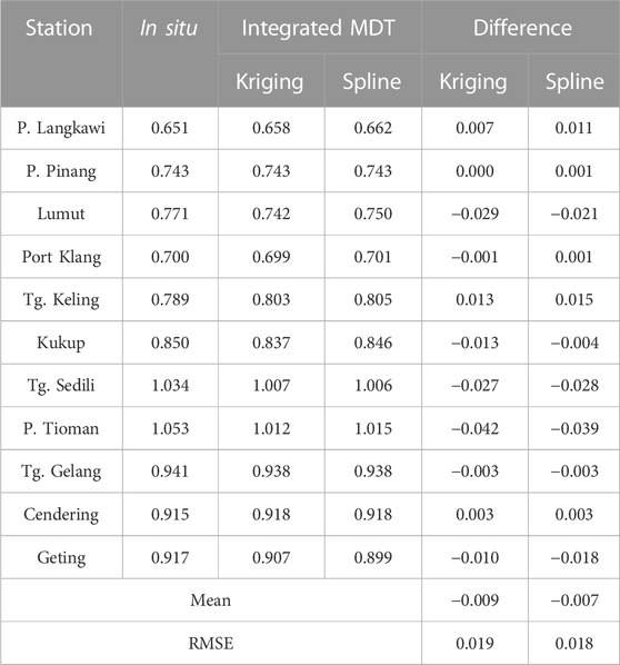
TABLE 5. Statistical results of differences between in situ and two interpolation MDT models [units are in meters].

These two interpolation MDT models are then combined with the MyGeoid_2017 model to develop a smooth continuous MSS model. To determine the best interpolation techniques in establishing the final integrated MSS, validations of these surfaces are carried out by comparing them with the input tide gauge values and the original altimetric UTM20 MSS. This comparison analysis is solely demonstrated to determine the accuracy of the interpolation procedures since no other known combined model spans within the study area for comparison. Table 6 displays the results of the comparison analysis. The integrated MSS models from ordinary kriging and minimum curvature methods have lower mean difference with in situ data of −0.003 m and −0.001 m, respectively, than the UTM20 MSS, which recorded −0.079 m. In addition, the accuracy of integrated MSS models also displays better agreement than pure altimetric MSS. In addition, ordinary kriging yields a slightly higher accuracy of 0.013 m than the minimum curvature spline technique with an accuracy of 0.014 m. Thus, the surface resulting from the ordinary kriging interpolation is selected as the final integrated MSS known as iUTM20. This demonstrates that the final integrated MSS closely matches the tide gauge values compared to UTM20 MSS, implying more accurate MSS in theory.

TABLE 6

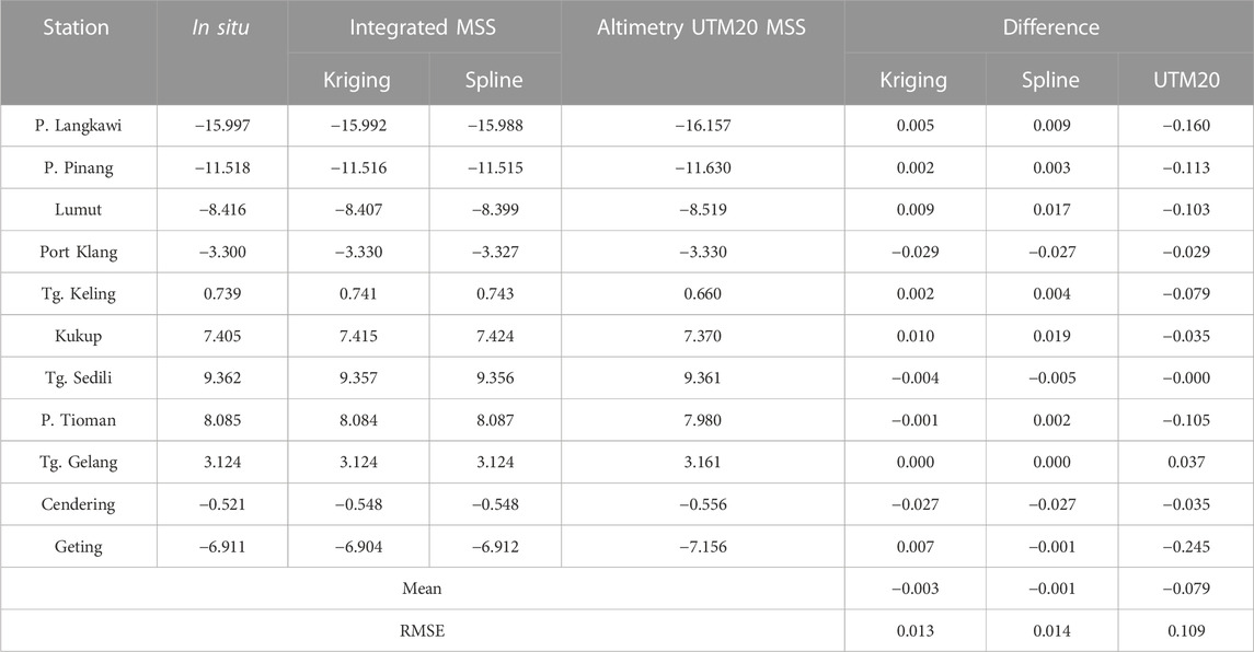
TABLE 6. Statistical analysis between ellipsoidal MSL and corresponding integrated MSS [units are in meters].

It is challenging to distinguish the difference between the integrated MSS and altimetric MSS patterns, as shown in Supplementary Figure S11. However, the integrated MSS has a better resolution and a distinct height pattern due to the assimilated tidal gauge data. The notable difference can be further examined through the statistical analysis shown in Table 7. Significant improvement is displayed from the integrated MSS model, where most of the differences at each tide gauge are below 10 cm compared to altimetric UTM20 MSS. In areas with no tide gauges, the integrated MSS cannot depend on its current form. Thus, increasing the density of tide gauge distribution is recommended to enhance the accuracy of the integrated MSS in this region. The final integrated MSS model, iUTM20 MSS, is illustrated in Figure 7. The integration can be enhanced when better and more tide gauge data became available, as it would be possible to analyze the spatial behavior of MSL between tide gauge data and satellite altimetry. Hence, it could improve the quality of the integration. Techniques adopted by other projects can be used or serve as a guide for Malaysia’s future techniques. For instance, VORF has adopted a combination of least-square collocation and specialized algorithms based on coastal topography to interpolate the reference surfaces between tide gauge and altimetry data (Iliffe et al., 2007). Other than that, the GNSS buoy surveys can be performed in the gap between tide gauge and altimetry data to estimate MSL relative to the ellipsoid and interpolate the datasets using the least-squares technique. This method is adopted by French BATHYELLI (Pineau-Guillou and Dorst, 2013).

TABLE 7

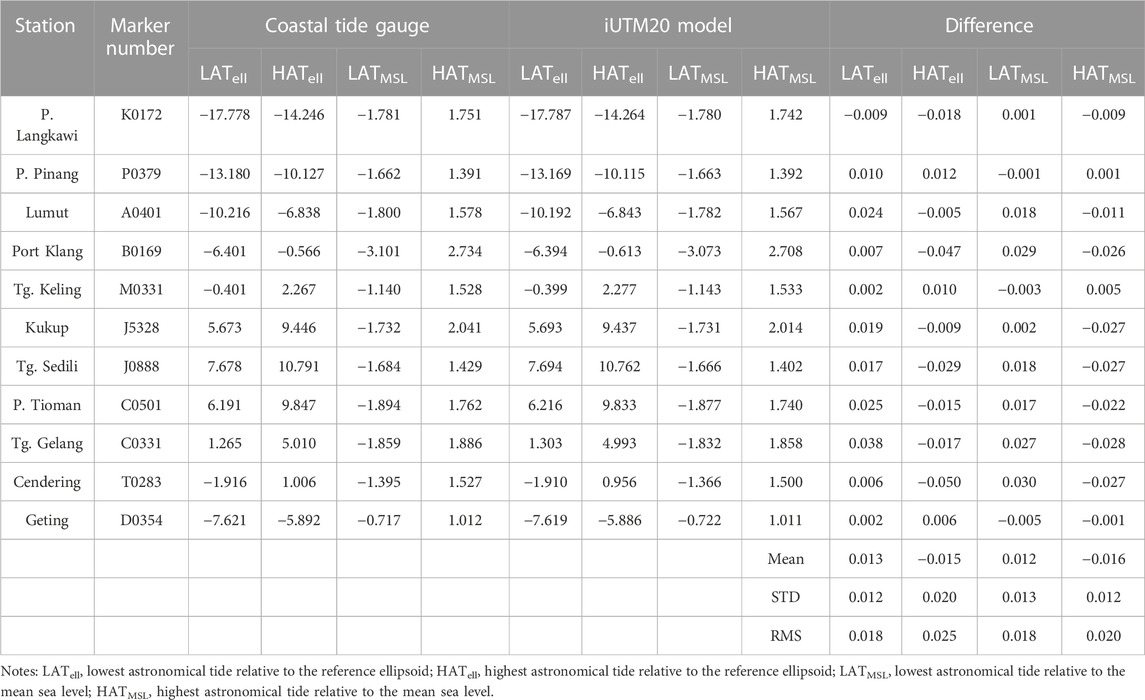
TABLE 7. Statistical results of the comparison between coastal tide gauge and continuous tidal datum separation surfaces [units are in meters].

FIGURE 7

FIGURE 7. Integrated iUTM20 MSS model.

3.6 Analysis of integrated UTM20 LAT and HAT

Integrated UTM20 LAT and HAT surfaces are the combination of the tide gauge data and altimetric-derived tidal modelling. Since the integration between tide gauges and altimetric-derived tidal datums is conducted along Peninsular Malaysia, the separation values in the other regions only depend on altimetric data. The results of LAT and HAT surfaces are shown in Figure 8. The figure clearly shows that the middle part of Malacca Strait has the lowest and the highest values of LAT and HAT, respectively. This indicates that this area has the optimal tidal range of sea level compared to other regions. In addition, there are closer contour lines at Malacca Strait, which indicate possible drastic changes in LAT and HAT values. This is probably influenced by the shape of Malacca Straits, which is narrow closed sea and shallow water.

FIGURE 8

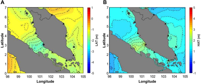
FIGURE 8. Surface model of tidal datums along with the Peninsular Malaysia region. (A) LAT is relative to MSL. (B) HAT is relative to MSL.

A gridded point of 1.5 min, with approximately 2.7 km spacing, is created over the study area to establish the ellipsoidal tidal datum separation surfaces. The space of the gridded point should be denser near the coastal area to capture the coastal variations. Unfortunately, this study did not adopt the hydrodynamic model along the coastal regions due to the intensive computational nature of estimating the model, and it requires a high-performance computing system. Each gridded tidal datum surface is added independently to the final integrated MSS, iUTM20 MSS, to generate gridded ellipsoidal tidal datum separation surfaces. The final statistics of tidal datum separations are tabulated in Table 7. The statistics indicate that the RMS agreements between the established LAT and HAT relative to MSL with coastal tide gauges are 1.8 cm and 2.0 cm, respectively. For the ellipsoidal LAT and HAT, the RMS agreements yield 1.8 cm and 2.5 cm, respectively. The findings also show that the iUTM20 tidal models have significant improvement compared to the difference of LAT_MSL and HAT_MSL, which only derived using altimetric data, as shown in Supplementary Table S8 and Supplementary Table S9, respectively. Since all the available data have been utilized to compute the surface, it has noted that the results are merely a measure of precision.

4 Conclusion

This paper presents several important results in developing continuous Malaysian VSEP models to realize the ERS technique. The Malaysian VSEP models consist of MSS/MSL, MDT, LAT, and HAT. These models have been developed by combining the offshore and coastal datasets, which are retrieved from satellite altimetry and coastal tide gauges, respectively. Prior to this, new regional UTM20 MSS, UTM20 MDT, UTM20 LAT, and UTM20 HAT models have been developed using satellite altimetry to represent the offshore datasets. UTM20 LAT and UTM20 HAT models are developed based on along-track SSH modelling using the harmonic analysis approach and interpolated using ordinary kriging and minimum curvature spline methods. Before performing the interpolation, the reliability of predicted along-track SSH is assessed by comparing with the observed along-track SSH. Then, these interpolation models are evaluated based on the statistical comparison with coastal tide gauges.

The results of the vertical datum at coastal tide gauges are also described in this paper. Hourly tidal data spanning more than 19 years are used to establish MSL by simple averaging. The outcomes of tide gauge-derived MDT are analyzed by computing the separation offset between MSL and MyGeoid_2017. Computation of LAT and HAT is obtained based on the analysis of filtered hourly tidal data using the harmonic analysis approach, and the accuracy of predicted tides ranges from 9.5 cm to 13.8 cm. From Tide Gauge GNSS Campaign 2019, all the developed vertical reference points at the DSMM coastal tide gauges along Peninsular Malaysia are shifted to the reference ellipsoid, and the results display good accuracy of GNSS latitude and longitude as well as ellipsoidal heights. The analysis of integrated UTM20 MDT and UTM20 MSS models is described in this paper, where the integration of the MDT model is conducted 10 km from the coastline to 20 km offshore for satellite altimetry. Ordinary kriging and minimum curvature spline methods are tested to interpolate the MDT model and establish the final integrated MSS. Based on the statistical analysis, the ordinary kriging method produces better results than the minimum curvature spline technique in establishing iUTM20 MDT and MSS models. However, the analysis of integrated iUTM20 LAT and HAT relative to MSL provides the opposite results where minimum curvature spline delivers better results than ordinary kriging.

The present study demonstrates that tidal datum modelling involves only mathematical interpolation of tidal datum heights derived from the available tide gauges. In general, this method is appropriate in the vicinity of primary tide gauges. VSEP models should be used in various applications that are related to marine applications, for which they should be stored in the database. It is suggested to incorporate the complex hydrodynamic model in developing the VSEP model as it can produce a reliable statistical model in areas where tide gauge is unavailable and with the factors of local control such as rivers or bays. Thus, by incorporating the complex hydrodynamic model, it can significantly improve the accuracy/reliability of the VSEP model in the future. Moreover, further assessment of the VSEP model must be carried out in the future to determine its reliability, specifically in the offshore area, as this paper can only assess the accuracy of the model over the coastal area. This is because, during this study, there exists limited resource to evaluate the accuracy of the model over the offshore region since we are unable to obtain tide gauge data from the authorities. It is hoped that future study can compensate the drawback.

Data availability statement

The original contributions presented in the study are included in the article/Supplementary Material; further inquiries can be directed to the corresponding author.

Author contributions

AD and DW conceived and designed the initial ideas for this study. MH carried out the designed experiments. MH and MP performed the data analysis. The manuscript was written by MH and NA with contributions from AD, DW, and AC. All authors contributed to the article and approved the submitted version.

Funding

This project was funded by the Ministry of Education Malaysia under the Fundamental Research Grant Scheme (FRGS) (FRGS/1/2020/WAB05/UTM/02/1) and Universiti Teknologi Malaysia for funding under the UTM Encouragement Research Grant (UTMER) (Q.J130000.3852.31J46).

Acknowledgments

The authors would like to express their gratitude to TU Delft, NOAA, and Altimetrics LLC for providing the altimetry data through the RADS Server. The authors would like to extend a special thanks to the Department of Survey and Mapping Malaysia (DSMM) for kindly contributing the local precise geoid model and tidal data for this study.

Conflict of interest

The authors declare that the research was conducted in the absence of any commercial or financial relationships that could be construed as a potential conflict of interest.

Publisher’s note

All claims expressed in this article are solely those of the authors and do not necessarily represent those of their affiliated organizations, or those of the publisher, the editors, and the reviewers. Any product that may be evaluated in this article, or claim that may be made by its manufacturer, is not guaranteed or endorsed by the publisher.

Supplementary material

The Supplementary Material for this article can be found online at: https://www.frontiersin.org/articles/10.3389/feart.2023.1110181/full#supplementary-material

References

Abazu, I. C., Din, A. H. M., and Omar, K. M. (2017). Mean dynamic topography over Peninsular Malaysian seas using multimission satellite altimetry. J. Appl. Remote Sens. 11 (2), 026017. doi:10.1117/1.JRS.11.026017

CrossRef Full Text | Google Scholar

Ainee, A. (2016). “Derivation of tidal constituents from satellite altimetry data for coastal vulnerability assessment in Malaysia,”. MSc Thesis (Skudai: Universiti Teknologi Malaysia).

Google Scholar

Alihan, N. S. A. (2018). “Estimation of geophysical loadings over the Malaysian region based on kinematic precise point positioning GPS technique,”. MSc Thesis (Skudai: Universiti Teknologi Malaysia).

Google Scholar

Alihan, N. S. A., Wijaya, D. D., Din, A. H. M., Bramanto, B., and Omar, A. H. (2019). “Spatiotemporal variations of Earth tidal displacement over peninsular Malaysia based on GPS observations,” in Lecture notes in civil engineering. Editor B. Pradhan 9 edn (Singapore: Springer), 806–823.

CrossRef Full Text | Google Scholar

Andersen, O. B., and Scharroo, R. (2011). “Range and geophysical corrections in coastal regions and implications for mean sea surface determination,” in Coastal altimetry. Editors S. Vignudelli, A. Kostianoy, P. Cipollini, and J. Benveniste (Springer), 103–114. doi:10.1007/978-3-642-12796-0_5

CrossRef Full Text | Google Scholar

Andersen, O., Knudsen, P., and Stenseng, L. (2018). “A new DTU18 MSS Mean Sea Surface – improvement from SAR altimetry,” in 25 Years of Progress in Radar Altimetry Symposium, Portugal, 24 Sept 2018 → 29 Sept 2018.

Google Scholar

Baqer, M. M. (2011). “Establishing and updating vertical datum for land and hydrographic surveying in what is vertical datum?,” in FIG Working Week 2011: Bridging the Gap between Cultures, Marrakech, Morocco, 18-22 May 2011.

Google Scholar

International Hydrographic Organization (IHO) (2005). Chapter 2 “positioning” in Publication C-13 manual on hydrography. Editor Bureau I. H. 1st Ed. (International Hydrographic Bureau), 33–117.

Google Scholar

Byun, D. S., and Hart, D. E. (2019). On robust multi-year tidal prediction using T_TIDE. Ocean Sci. J. 54 (4), 657–671. doi:10.1007/s12601-019-0036-4

CrossRef Full Text | Google Scholar

Daher, V. B., Paes, R. C. V., França, G. B., Alvarenga, J. B. R., and Teixeira, G. L. G. (2015). Extraction of tide constituents by harmonic analysis using altimetry satellite data in the Brazilian coast. J. Atmos. Ocean. Technol. 32 (3), 614–626. doi:10.1175/JTECH-D-14-00091.1

CrossRef Full Text | Google Scholar

Deng, X., Featherstone, W. E., Hwang, C., and Berry, P. A. M. (2002). Estimation of contamination of ERS-2 and POSEIDON satellite radar altimetry close to the coasts of Australia. Mar. Geod. 25 (4), 249–271. doi:10.1080/01490410214990

CrossRef Full Text | Google Scholar

Department of Survey and Mapping Malaysia (DSMM) (2005). Garis panduan penggunaan model geoid Malaysia (MYGEOID). In KPUP circular 10/2005 (vol. 148, issue september). Available at: https://www.jupem.gov.my/v1/wp-content/uploads/2016/04/Survey-General-Circular-Vol.-10-2005-on-MyGEOID.pdf.

Google Scholar

Dibarboure, G., Renaudie, C., Pujol, M. I., Labroue, S., and Picot, N. (2012). A demonstration of the potential of Cryosat-2 to contribute to mesoscale observation. Adv. Space Res. 50 (8), 1046–1061. doi:10.1016/j.asr.2011.07.002

CrossRef Full Text | Google Scholar

Din, A. H. M., Hamid, A. I. A., Yazid, N. M., Tugi, A., Khalid, N. F., Omar, K. M., et al. (2017). Malaysian sea water level pattern derived from 19 years tidal data. J. Teknol. 79 (5), 137–145. doi:10.11113/jt.v79.9908

CrossRef Full Text | Google Scholar

Dodd, D., and Mills, J. (2011). “Ellipsoidally referenced surveys (ERS); issues and solutions,” in Proceedings of the U.S. Hydro 2011 Conference, Tampa, Florida, USA, 25-28 April, 2011.

Google Scholar

Dodd, D., and Mills, J. (2012). “Ellipsoidally referenced surveys separation models,” in FIG Working Week 2012, Knowing to Manage the Territory, Protect the Environment, Evaluate the Cultural Heritage, Rome, Italy, 6-10 May 2012, 1–20.

Google Scholar

Doyle, D. (2007). Vertical datum. New mapping studies Convert to updated vertical datum. U.S. Department of Homeland Security. July, 1–3.

Google Scholar

Ekman, M. (1989). Impacts of geodynamic phenomena on systems for height and gravity. Bull. Géodésique 63 (1), 281–296. doi:10.1007/bf02520477

CrossRef Full Text | Google Scholar

Farrell, S. L., McAdoo, D. C., Laxon, S. W., Zwally, H. J., Yi, D., Ridout, A., et al. (2012). Mean dynamic topography of the arctic ocean. Geophys. Res. Lett. 39 (1), 1601. doi:10.1029/2011GL050052

CrossRef Full Text | Google Scholar

Fisher, R., Perkins, S., Walker, A., and Wolfart, E. (2003). Spatial Filters – Gaussian Smoothing. Available at: https://homepages.inf.ed.ac.uk/rbf/HIPR2/gsmooth.htm (Accessed October 30, 2020). doi:10.2172/814025

CrossRef Full Text | Google Scholar

Fok, H. S. (2012). “Ocean tides modeling using satellite altimetry,”. Doctoral dissertation (The Ohio State University).

Google Scholar

Fu, Y., Zhou, D., Zhou, X., Sun, Y., Li, F., and Sun, W. (2020). Evaluation of satellite-derived tidal constituents in the South China Sea by adopting the most suitable geophysical correction models. J. Oceanogr. 76 (3), 183–196. doi:10.1007/s10872-019-00537-2

CrossRef Full Text | Google Scholar

Gill, S. K., and Porter, D. L. (1980). Theoretical offshore tide range derived from a simple defant tidal model compared with observed offshore tides. Int. Hydrogr. Rev. 57 (1).

Google Scholar

Guo, M., Xiu, P., Chai, F., and Xue, H. (2019). Mesoscale and submesoscale contributions to high Sea Surface chlorophyll in subtropical gyres. Geophys. Res. Lett. 46 (22), 13217–13226. doi:10.1029/2019GL085278

CrossRef Full Text | Google Scholar

Hamden, M. H., and Din, A. H. M. (2018). A review of advancement of hydrographic surveying towards ellipsoidal referenced surveying technique. IOP Conf. Ser. Earth Environ. Sci. 169 (1), 12019. doi:10.1088/1755-1315/169/1/012019

CrossRef Full Text | Google Scholar

Hamden, M. H., Din, A. H. M., and Pa’suya, M. F. (2019). “Assessment of Sea Level variability from multi-mission satellite altimetry in coastal zone,” in GBES Conference Proceedings, Malaysia, Johor, 24th - 25th June 2019 (Faculty of Built Environment and Surveying, UTM), 73–80.

Google Scholar

Hamden, M. H., Din, A. H. M., Wijaya, D. D., Yusoff, M. Y. M., and Pa’Suya, M. F. (2021). Regional Mean Sea Surface and mean dynamic topography models around Malaysian seas developed from 27 Years of along-track multi-mission satellite altimetry data. Front. Earth Sci. 9, 1–16. doi:10.3389/feart.2021.665876

CrossRef Full Text | Google Scholar

Iliffe, J. C., Ziebart, M. K., and Turner, J. F. (2007). The derivation of vertical datum surfaces for hydrographic applications. Hydrogr. J. 125, 3–8.

Google Scholar

Iliffe, J. C., Ziebart, M. K., Turner, J. F., Talbot, A. J., and Lessnoff, A. P. (2013). Accuracy of vertical datum surfaces in coastal and offshore zones. Survey Review 45 (331), 254–262. doi:10.1179/1752270613Y.0000000040

CrossRef Full Text | Google Scholar

International Hydrographic Organization (IHO) (2018). Resolutions of the international hydrographic organization (A2.5 3/191, issue 377. MONACO: International Hydrographic Organization. Available at: http://www.iho.int/iho_pubs/misc/M1Eversion07.pdf.

Google Scholar

Jamil, H., Kadir, M., Forsberg, R., Olesen, A., Isa, M. N., Rasidi, S., et al. (2017). Airborne geoid mapping of land and sea areas of East Malaysia. J. Geod. Sci. 7 (1), 84–93. doi:10.1515/jogs-2017-0010

CrossRef Full Text | Google Scholar

Jin, T., Li, J., and Jiang, W. (2016). The global mean sea surface model WHU2013. Geod. Geodyn. 7 (3), 202–209. doi:10.1016/j.geog.2016.04.006

CrossRef Full Text | Google Scholar

Keysers, J. H., Quadros, N. D., and Collier, P. A. (2013). Developing a method to establish a common vertical datum before integrating land height data with nearshore seafloor depth data.

Google Scholar

Keysers, J. H., Quadros, N. D., and Collier, P. A. (2015). Vertical datum transformations across the Australian littoral zone. J. Coast. Res. 299, 119–128. doi:10.2112/JCOASTRES-D-12-00228.1

CrossRef Full Text | Google Scholar

Klein, P., Lapeyre, G., Siegelman, L., Qiu, B., Fu, L. L., Torres, H., et al. (2019). Ocean-scale interactions from space. Earth Space Sci. 6 (5), 795–817. doi:10.1029/2018EA000492

CrossRef Full Text | Google Scholar

Knudsen, P., and Andersen, O. B. (2013). The DTU12MDT global mean dynamic topography and ocean circulation. Model. Proc. ESA Living Planet Symposium 722 (December), 28. http://earth.esa.int/gut/

Google Scholar

Lee, H., Choi, Y., Ham, G., and Yun, S. (2017). “Experimental assessment of achievable accuracy of GNSS-derived heights from carrier phase-based positioning techniques for ellipsoidally referenced hydrographic surveys,” in FIG Working Week 2017, Surveying the World of Tomorrow - From Digitalisation to Augmented Reality, Helsinki, Finland, May 29–June 2, 2017, 8792.

Google Scholar

Lindsley, R. D. (2013). Fitting tidal constituents to altimeter data, 1–5.

Google Scholar

Losch, M., Snaith, H., Siegismund, F., and Knudsen, P. (2007). “GOCE user toolbox specification: scientific trade off study and algorithm specification,” in 3rd International GOCE User Workshop, Frascati, Italy, 06-Nov - 08-Nov 2006 (European Space Agency, (Special Publication) ESA SP, SP-627), 303–310.

Google Scholar

Mahyudin, R., Din, A. H. M., and Hamden, M. H. (2019). “Localized mean dynamic topography model,” in Geoinformation Technology for Malaysian seas. Editors N. H. Idris, and A. W. Rasib (Universiti Teknologi Malaysia: Penerbit UTM Press), 129–143.

Google Scholar

Mills, J., and Dodd, D. (2014). Ellipsoidally referenced surveying for hydrography. International Federation of Surveyor. (FIG) (Issue 62). FIG.

Google Scholar

Mohamed, A. (2003). “An investigation of the vertical control network in peninsular Malaysia using a combination of levelling, gravity, GPS and tidal data,”. PhD Thesis (Skudai: Universiti Teknologi Malaysia).

Google Scholar

Mohamed, A. (2019). “Marine geodetic modernisation in Malaysian waters: current development and future direction,” in KL Geohydro 2019 “Empowering Marine Knowledge Through Hydrography, Kuala Lumpur, Malaysia, 18-19 November 2019, 16.

Google Scholar

Munk, W. H., and Cartwright, D. E. (1966). Tidal spectroscopy and prediction. Philosophical Trans. R. Soc. Lond. Ser. A, Math. Phys. Sci. 259, 533–581. doi:10.1098/rsta.1966.0024

CrossRef Full Text | Google Scholar

Nanlal, C., Miller, K., Davis, D., and Sutherland, M. (2020). Establishing vertical separation models for vulnerable coastlines in developing territories. Mar. Geod. 44 (0), 387–407. doi:10.1080/01490419.2020.1844825

CrossRef Full Text | Google Scholar

National Oceanic and Atmospheric Administration (NOAA) (2017). Vertical datums. National geodetic survey. National geodetic survey. Available at: www.ngs.noaa.gov/datums/vertical/ (Accessed March 14, 2018).

Google Scholar

Pa’suya, M. F. (2020). “New modern height reference system for peninsular Malaysia using least square modification of Stokes’ formula,”. PhD Thesis (Skudai: Universiti Teknologi Malaysia).

Google Scholar

Pineau-Guillou, L., and Dorst, L. (2013). “Creation of vertical reference surfaces at sea using altimetry and GPS,” in Reference frames for applications in geosciences, international association of geodesy symposia vol. 138. Editors Z. Altamimi, X. Collilieux, and L. Metivier (Springer Science and Business Media), 137–145. Available at: http://www.scopus.com/inward/record.url?eid=2-s2.0-84884346250&partnerID=tZOtx3y1.

CrossRef Full Text | Google Scholar

Pirooznia, M., Emadi, S. R., and Alamdari, M. N. (2016). The time series spectral analysis of satellite altimetry and coastal tide gauges and tide modeling in the coast of caspian sea. Open J. Mar. Sci. 06 (02), 258–269. doi:10.4236/ojms.2016.62021

CrossRef Full Text | Google Scholar

Pujol, M., Schaeffer, P., Faugère, Y., Raynal, M., Dibarboure, G., and Picot, N. (2018). Gauging the improvement of recent Mean Sea Surface models: A new approach for identifying and quantifying their errors. Geophys. Res. Oceans 123 (8), 5889–5911. doi:10.1029/2017JC013503

CrossRef Full Text | Google Scholar

Quality Positioning Services (QPS) (2020). International terrestrial reference frame 2014 (ITRF2014). How-To geodetic items. Available at: https://confluence.qps.nl/qinsy/latest/en/international-terrestrial-reference-frame-2014-itrf2014-182618383.html (Accessed January 1, 2020).

Google Scholar

Reguzzoni, M., Carrion, D., Iapige De Gaetani, C., Albertella, A., Rossi, L., Sona, G., et al. (2021). Open access to regional geoid models: the International Service for the Geoid. Earth Syst. Sci. Data 13 (4), 1653–1666. doi:10.5194/essd-13-1653-2021

CrossRef Full Text | Google Scholar

Rice, G., and Riley, J. (2011). Measuring the water level datum relative to the ellipsoid during Hydrographic survey. [Online]. Available at: http://ushydro.thsoa.org/hy11/0427A_08.pdf.

Google Scholar

Schaeffer, P., Faugére, Y., Legeais, J. F., Ollivier, A., Guinle, T., and Picot, N. (2012). The CNES_CLS11 global mean sea surface computed from 16 years of satellite altimeter data. Mar. Geod. 35(sup1), 3–19. doi:10.1080/01490419.2012.718231

CrossRef Full Text | Google Scholar

Siegel, D. A., McGillicuddy, D. J., and Fields, E. A. (1999). Mesoscale eddies, satellite altimetry, and new production in the Sargasso Sea. J. Geophys. Res. Oceans 104 (C6), 13359–13379. doi:10.1029/1999jc900051

CrossRef Full Text | Google Scholar

Simons, W., Naeije, M., Ghazali, Z., Rahman, W. D., Cob, S., Kadir, M., et al. (2023). Relative sea level trends for the coastal areas of peninsular and east malaysia based on remote and in situ observations. Remote Sensing 15(4), 1113. doi:10.3390/rs15041113

CrossRef Full Text | Google Scholar

Teo, C. H., and Fauzi, A. (2006). “A national geocentric datum and the administration of marine spaces in Malaysia,” in FIG publication 36: Administering marine spaces - international issues. FIG commissions 4 and 7 working Group 4.3 (FIG).

Google Scholar

Terry, H. (2004). ICESat/GLAS and WGS-84 ellipsoid and geoid conversions. http://nsidc.org/data/icesat/faq.html#p9.

Google Scholar

Turner, J. F., Iliffe, J. C., Ziebart, M. K., Wilson, C., and Horsburgh, K. J. (2010). Interpolation of tidal levels in the coastal zone for the creation of a hydrographic datum. J. Atmos. Ocean. Technol. 27 (3), 605–613. doi:10.1175/2009JTECHO645.1

CrossRef Full Text | Google Scholar

Wijaya, D. D. (2012). Pengantar fourier series. Unpublished note, kelompok keilmuan geodesi. Indonesia: Institut Teknologi Bandung.

Google Scholar

Wöppelmann, G., and Marcos, M. (2016). Vertical land motion as a key to understanding sea level change and variability. Rev. Geophys. 54 (1), 64–92. doi:10.1002/2015rg000502

CrossRef Full Text | Google Scholar

Yahaya, N. A. Z., Musa, T. A., Omar, K. M., Din, A. H. M., Omar, A. H., Tugi, A., et al. (2016). Mean sea surface (MSS) model determination for Malaysian seas using multi-mission satellite altimeter. Int. Archives Photogrammetry, Remote Sens. Spatial Inf. Sci. - ISPRS Archives 42 (4), 247–252. doi:10.5194/isprs-archives-XLII-4-W1-247-2016

CrossRef Full Text | Google Scholar

Yazid, N. (2018). “Marine geoid determination over Malaysian seas using satellite altimeter and gravity missions,”. MSc Thesis (Skudai: Universiti Teknologi Malaysia).

Google Scholar

Yuan, J., Guo, J., Liu, X., Zhu, C., Niu, Y., Li, Z., et al. (2020). Mean sea surface model over China seas and its adjacent ocean established with the 19-year moving average method from multi-satellite altimeter data. Cont. Shelf Res. 192, 104009. doi:10.1016/j.csr.2019.104009

CrossRef Full Text | Google Scholar

Yun, S., Lee, H., Choi, Y., and Ham, G. (2017). Potential accuracy of GNSS PPP- and PPK-derived heights for ellipsoidally referenced hydrographic surveys: experimental assessment and results. J. Position. Navigation, Timing 6 (4), 211–221. doi:10.11003/JPNT.2017.6.4.211

CrossRef Full Text | Google Scholar

Zulkifle, M. I., Din, A. H. M., Hamden, M. H., and Adzmi, N. H. M. (2019). Determination of a localized mean sea surface model for Malaysian seas using multi-mission Satellite Altimeter. ASM Sci. J. 12 (2), 81–89.

Google Scholar