 Yan Ji
 Xiefei Zhi
 Ying Wu3
 Luying Ji
- 1Collaborative Innovation Center on Forecast and Evaluation of Meteorological Disasters (CIC-FEMD)/Key Laboratory of Meteorological Disasters, Ministry of Education (KLME), Nanjing University of Information Science and Technology, Nanjing, China
- 2Weather Online Institute of Meteorological Applications, Wuxi, China
- 3Taizhou Environmental Monitoring Center, Taizhou, China
- 4Department of Environmental Occupational Hygiene, Taizhou Center for Disease Control and Prevention, Taizhou, China
- 5Key Laboratory of Transportation Meteorology of China Meteorological Administration, Nanjing Joint Institute for Atmospheric Sciences, Nanjing, China
Air pollution is of high relevance to human health. In this study, multiple machine-learning (ML) models—linear regression, random forest (RF), AdaBoost, and neural networks (NNs)—were used to explore the potential impacts of air-pollutant concentrations on the incidence of pediatric respiratory diseases in Taizhou, China. A number of explainable artificial intelligence (XAI) methods were further applied to analyze the model outputs and quantify the feature importance. Our results demonstrate that there are significant seasonal variations both in the numbers of pediatric respiratory outpatients and the concentrations of air pollutants. The concentrations of NO2, CO, and particulate matter (PM10 and PM2.5), as well as the numbers of outpatients, reach their peak values in the winter. This indicates that air pollution is a major factor in pediatric respiratory diseases. The results of the regression models show that ML methods can capture the trends and turning points of clinic visits, and the non-linear models were superior to the linear ones. Among them, the RF model served as the best-performing model. The analysis on the RF model by XAI found that AQI, O3, PM10, and the current month are the most important predictors affecting the numbers of pediatric respiratory outpatients. This shows that the number of outpatients rises with an increasing AQI, especially with the increasing of particulate matter. Our study indicates that ML models with XAI methods are promising for revealing the underlying impacts of air pollution on the pediatric respiratory diseases, which further assists the health-related decision-making.
1 Introduction
Since the reform and opening up of China from the 1980s, there have been significant achievements in its economy and the construction of infrastructure. However, the environmental problems caused by the extensive development model in the early stages is becoming a serious issue (Xu et al., 2013; Qi et al., 2020), especially regarding air pollution. Due to the rapid development of heavy industry, the continuous expansion of urbanization, and the sudden surge in the number of motor vehicles, the increasing emission of air pollutants is being monitored (Kan et al., 2012; Xu et al., 2013; Gu et al., 2020). In recent years, air pollution has been considered by the World Health Organization (WHO) as the greatest environmental risk to health (World Health Organization, 2021). Reports show that 90% of people are breathing polluted air every day (World Health Organization, 2018a). There are nearly 7 million premature deaths from cancer, strokes, and cardiopulmonary diseases caused by air pollution, and 90% of these deaths occur in low- and middle-income countries (World Health Organization, 2018b).
Studies have shown that the content of air pollutants significantly affects human health, both in the short and long term (Shahi et al., 2014; Khaniabadi et al., 2017; Song et al., 2018; Wang L. et al., 2018a; Song et al., 2019). The short-term effects are characterized by a rapid increase in the incidence of respiratory diseases, especially in vulnerable groups such as the elderly, children, and pregnant women (Sarnat et al., 2012; MacIntyre et al., 2014; Zhu et al., 2017; Li et al., 2018). WHO points it out that the particulate matter can penetrate into the lungs and enter the bloodstream, which further cause cardiovascular and respiratory impacts (World Health Organization, 2021). Besides, There is emerging evidence that NO2 is associated with respiratory diseases, i.e. asthma, coughing, and difficulty breathing (World Health Organization, 2022). Long-term chronic effects of air pollution are also seen on human health (Zhang et al., 2014; Islam et al., 2017). The Global Burden of Disease Study 2015 showed that chronic respiratory diseases ranked third among the fatal diseases in China, second only to cardiovascular and cerebrovascular diseases and tumors; all three of these types of disease are highly related to air pollution (Prüss-Üstün et al., 2016).
It is clear that air pollution is becoming one of the most important risk factors affecting human health. Specifically, a large number of studies have been performed examining the impact of air pollutants on the incidence of respiratory diseases in major cities across China (Wang and Chau, 2013; Wang L. et al., 2018a). It has been found that the air quality index (AQI) is positively correlated with bronchial infections, upper respiratory-tract infections, and lung diseases in Tianjin (Guo et al., 2010). Yin et al. (2011) pointed out that levels of particulate matter (PM2.5 and PM10), NO2, SO2, and carbon monoxide (CO) have positive correlations with the number of pediatric outpatients with respiratory diseases in Shanghai, while the correlation with ozone (O3) was negative. A case study by Zhang et al. (2014) showed that short-term exposure to air pollutants can cause explosive increases in pediatric patients with pneumonia in Guangzhou. The results of the study by Shen et al. (2017) showed that sulfur dioxide (SO2) is the main pathogenic factor for respiratory-tract infections in Henan Province, and this has synergistic effects with the particulate matter and nitrogen oxides (NOx). A study in Beijing further showed that air pollution is one of the important causes of the increase in the number of elderly patients with allergic rhinitis (Zhang et al., 2016).
The above studies clearly point out that the content of air pollutants can significantly affect the incidence of respiratory diseases. However, these studies were mainly based on parametric linear models, i.e., multiple linear regression, (Ruckerl et al., 2006; Wang M. et al., 2018b), or they relied on semi-parametric generalized linear models and generalized additive models (Dominici et al., 2002; Terzi and Cengiz, 2009; Ravindra et al., 2019). Unfortunately, these linear models are not very efficient for capturing the non-linear dependence among the complex data. Furthermore, although the regression coefficient can be simply used for evaluating the feature importance, it is incapable of quantifying the synergy of multiple variables and performing a local analysis for a given sample with the linear models.
The development of machine learning (ML) and deep learning has led to technological innovations in numerous areas, including autonomous driving (Bojarski et al., 2016; Badue et al., 2021), facial recognition (Hu et al., 2015; Parkhi et al., 2015), weather forecasting (McGovern et al., 2017; Reichstein et al., 2019), and smart healthcare (Litjens et al., 2017; Hesamian et al., 2019). Using a variety of linear and non-linear computational units, ML approaches are able to learn complex representative features from high-dimension data to establish models projecting from predictors to predictands. In the field of the atmospheric environment, a number of studies have been performed considering time-series prediction of atmospheric pollutants (Freeman et al., 2018; Wang et al., 2020; Kleinert et al., 2022), spatial and temporal downscaling (Yu and Liu, 2021; Geiss et al., 2022), and modal classification (Harrou et al., 2018). However, there have still been few studies using ML models with explainable artificial intelligence (XAI) methods to analyze the correlations between air-pollutant concentrations and human health. Because ML models have higher non-linearity and stronger robustness, it is of great significance to simulate how the morbidity rates of respiratory diseases are affected by the concentrations of different air pollutants. Furthermore, XAI methods can further quantitatively analyze the feature importance of each air-pollutant input and help to reveal the underlying impacts of air pollution on human health.
Taizhou is an important part of the Yangtze River Delta Economic Zone in East China, with inland ports and mature industries. However, it still suffers from the growing problem of air pollution in its main urban area. This is largely caused by the chemical industry, automobile exhaust emissions, construction-site dust, and transmission of pollutants. More seriously, measurements further show that the air pollution issue in Taizhou is more prominent among the surrounding cities and few studies are performed for assessing the impacts of air pollution on human health in Taizhou city. In this context, exploring the impact of air quality on the incidence of pediatric respiratory diseases is of great social significance. In this study, we aimed to carry out a risk assessment of air pollution on children’s health in Taizhou with ML models and provide a scientific basis for taking effective intervention measures. In this work, the impact of the air pollution was characterized by changes in the number of pediatric patients visiting respiratory departments; furthermore, XAI methods were used to analyze the contribution of the content of the air pollutants. The main contributions of our study can be summarized as follows: 1. A detailed statistical analysis is performed between the air-pollutant concentrations and the number of pediatric respiratory outpatients in Taizhou, i.e. detrended correlation analysis, stratified analyses by seasons, air-pollution levels, and types of primary pollutant. 2. XAI methods are introduced to evaluate the ML model performance in simulating the number of the clinic visits, by quantifying the feature importance of the air-pollutant factors. 3. It is a useful complement to the research of regional air quality and pediatric respiratory diseases using XAI and ML methods in Taizhou city.
The remainder of this manuscript is organized as follows. Section 2 introduces the clinical and air-pollutant monitoring data used in our work, as well as the ML models and XAI methods. Summary and detailed results are presented in Section 3, and this is followed by conclusions and future outlook in Section 4.
2 Data and methods
2.1 Data and preprocessing
The datasets used in this work included daily air-pollutant monitoring data from the Taizhou Environmental Monitoring Center and daily clinical data from the pediatric department of a comprehensive Grade 3A hospital in the urban area of Taizhou, spanning from 2018 to 2020. The air-pollutant data covers measurements of the content of PM2.5, PM10, CO, NO2, SO2, and O3, as well as the AQI, the level of air pollution, and the type of primary pollutant. The clinical data is the total number of outpatients visiting the pediatric department each day. Since the daily number of outpatients was found to follow a Poisson distribution using the Kolmogorov–Smirnov test, a log transform was further applied to the raw clinical data. Given the raw clinical data as Ct, the preprocessed predicant Yt is:
where the subscript t is the timestamp of the sample.
In this study, in addition to the measurements of air pollutants, temporal information was also used as an additional predictor. Hence, the candidate predictors Xt consist of PM2.5, PM10, CO, NO2, SO2, and O3, as well as AQI, the level of air pollution (AQI_level), the type of primary pollutant (Major_pollutant), and temporal information (Month). AQI_level consists of four categories from I to IV; the higher the AQI_level, the worse the air quality. Major_pollutant indicates the type of primary pollutant. In our study, Major_pollutant I means that there is no air pollution. Major_pollutant values from II to VII were defined as the cases of O3, CO, NO2, SO2, PM10, and PM2.5, respectively being the primary pollutant. The temporal information is the month of the given sample.
2.2 ML models
The ML models used in this study included linear regression, ridge regression, Huber regression, random forest (RF), adaptive boosting (AdaBoost), and a neural network (NN). Among these, linear regression, ridge regression, and Huber regression are considered as weakly non-linear models, while RF, AdaBoost, and NN are more robust and complex.
Linear regression is one of the most basic statistical models. Given predictors X = {x1, x2, …, xk}, the prediction
where W = {w0, w1, w2, …, wk} are the regression coefficients (weights) of the corresponding predictors. The weights are usually estimated by optimizing the L2 loss:
where y is the ground truth. However, linear regression models are sensitive to outliers and are hence highly dependent on reliable feature engineering. To build a more robust model, ridge regression (Hoerl and Kennard, 1970) and Huber regression (Huber, 1973) further add regularization terms into the loss function. The loss function of ridge regression can be written as:
where α ≥ 0 is the penalty coefficient. A larger α means stronger regularization on the model. Huber regression pays more attention to handling outliers. The loss is given as:
where
in which δ and ϵ are the non-negative constant parameters.
A decision tree is a classic non-parametric supervised learning approach; a tree-like model is built to learn the simple rules inferred from the data features, and this has multiple nodes and branches. The clear structure of a decision tree makes it easy to understand, and it is hence commonly used in data science and decision-making. An RF (Breiman, 2001) is an ensemble of decision trees. It consists of a number of independent decision trees; each decision tree is trained with random bootstrapped samples, and each node of the decision tree is estimated using random combinations of predictor variables. The ensemble mean of the decision trees is used as the prediction of the RF model, and this helps to improve accuracy and mitigate overfitting problems.
AdaBoost (Freund and Schapire, 1997) is another commonly used ensemble machine model. It starts with an initial weak learner, i.e., a linear model, and this weak learner is trained with the complete dataset to obtain an accuracy that is slightly higher than random guessing. Then, AdaBoost reweights the training samples and assigns higher weights to the samples misclassified by the initial weak learner. Subsequently, the goal of AdaBoost is to build another weak learner to complement the previous one with these reweighted training samples. In this adaptive strategy, the training samples misclassified by the previous weak learner will contribute more to the model performance, and hence the subsequent weak learners are forced to improve the misclassified samples. The final AdaBoost model is an ensemble of all the individual weak learners that converges to a strong learner.
As a more flexible and non-linear ML method, NNs (Rumelhart et al., 1986) have been widely used in multiple fields including computer vision, earth science, and biological science. These are built from multiple layers, and each layer consists of a number of neural nodes with non-linear activation functions. The prediction of an NN model is generated through forward propagation. A loss function is applied to quantify the distance between the model output and the ground truth. A series of optimizers have been designed to minimize the loss function using backward propagation with the training samples. Hence, NNs are highly non-linear and they have advantages in learning representative features from the data. However, a decrease in model performance is seen when handling a small dataset with an NN.
2.3 Explainable artificial intelligence methods
Although ML models show great potential for improved performance, there are always questions relating to how their decisions are made and how much we can rely on them. Hence, it is of great importance to understand the results of ML models rather than them simply being “black boxes.” In this study, four XAI methods—permutation feature importance (PFI), the partial dependence plot (PDP), local interpretable model-agnostic explanations (LIME), and Shapley additive explanations (SHAP)—are used to gain a well-grounded understanding of the established ML models and explore the feature importance of their predictors.
The PFI method (Breiman, 2001) computes the contribution of a single feature by randomly shuffling its values among the validation/testing samples with a trained model while keeping the other features unchanged. The decrease in the model score, i.e., R2 for regression, with the permuted data is defined as the importance of the selected feature. Since the model and the remaining features are unchanged, the change in the model’s score is seen as the contribution of that feature to the model performance. It can be seen that the PFI strategy can be applied to any ML model because it gives the feature importance by simply permuting the data without internal knowledge of model that has been used. Given an ML model f trained with data containing K features, the model score evaluated on the unpermuted testing data D is s. Then, a random permutation is performed on feature k among the testing samples to obtain the permuted data
In practice, Ik is computed multiple times on different perturbed data, and the average value is used as the feature importance. The larger the value of Ik, the more significant the impact of the feature on the prediction and the more important the feature.
The PDP (Friedman, 2001) is used to assess the marginal effects of one or two features in an ML model. The idea is similar to the PFI method, in that the feature importance is defined as the drop in the model score that occurs when breaking the relationship between the given feature and targets. The strategy of the PDP is to calculate the importance of the given feature by marginalizing over the distribution of the other features among the training data. Given an ML model f trained with data D containing K features, the set of features we are interested in is k (usually one or two features) and the set of remaining features is c. The partial dependence function is then given as:
In practice, the partial dependence function is estimated as:
where n is the number of instances in the training data, xk is the value of feature k, and xc is the actual values of the remaining features in set c. The partial dependence
Both the PFI and PDP methods evaluate the global contribution of a feature to the model prediction. However, in many cases, we are more interested in how the features affect the model’s decision in a given instance. Here, LIME (Ribeiro et al., 2016) serves as an XAI method for the local explanations for agnostic models; this further helps to understand the ways in which ML models make their predictions. The basic idea of LIME is to train an interpretable model as a good approximation of the original ML model locally. Given an ML model f trained with data D containing K features, the predictions of f for sample Di are f (Di). To understand the prediction f (Di), LIME generates a new dataset
SHAP (Lundberg and Lee, 2017) gives another solution to explain the individual predictions of ML models based on the Shapley values (Shapley, 1997) in coalitional game theory. The Shapley values are used to fairly assess the contribution of each feature to the model prediction. In coalitional game theory, the effect of a feature should not be evaluated alone but on all the possible coalitions of features. Given an ML model f with training data D containing K features, the number of possible combinations of features is 2K − 1. Using each combination as the input of the trained model f, there are 2K − 1 predictions, and the differences between these predictions and the original predictions using the complete set of features are calculated as the contributions of the combined features. The average marginal effect of a feature across all possible coalitions is defined as the Shapley value. However, in real applications, it is very time-consuming to calculate all these coalitions. Hence, Lundberg and Lee (2017) combined the LIME and Shapley values and further proposed an alternative estimation method, SHAP, based on the kernel and tree models. SHAP is computationally efficient and can be used for both global and local interpretation.
3 Results
3.1 Overview of the air-pollutant concentrations and the number of pediatric respiratory outpatients in Taizhou
Figure 1 shows the distribution and the trend in the number of patients visiting the pediatric department of a comprehensive Grade 3A hospital in Taizhou from 2018 to 2020. It can be seen that respiratory-related diseases account for over 60% of all diseases in the pediatric department, and there are clear interannual and seasonal variations. In particular, the number of pediatric respiratory outpatients in 2019 was significantly higher than in 2018 and 2020, with a peak occurring in the winter. Could this difference be related to the emission of air pollution?
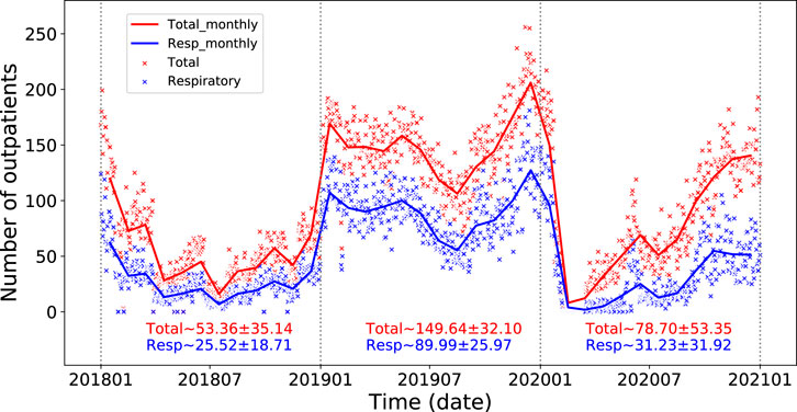
FIGURE 1. Time series of the numbers of patients visiting the pediatric department of a comprehensive Grade 3A hospital in Taizhou from 2018 to 2020. The scatter points show the number of pediatric outpatients (red) and outpatients visiting for respiratory diseases (blue) in a single day. The solid lines are the monthly average respectively. The mean and standard deviation for each year are shown at the bottom of the plot.
The statistics of the air-pollutant concentrations are shown in Figure 2. A remarkable decline is seen in most of the air-pollutant concentrations from 2018 to 2020, although there is a slight increase in O3. This indicates that the measures implemented to control air pollution in Taizhou have resulted in some progress, especially for the emission of SO2, PM2.5, and PM10. The results also show that there is significant seasonal variation in the relative proportions of the air pollutants. The concentrations of NO2, CO, PM2.5, and PM10 are at their peak in winter and low in summer, which is opposite to the trend for O3. The main reason for the high concentrations of NO2, CO, and PM in winter is the increased heating needs of residents; this causes an increase in the amount of coal being burned. The high concentration of O3 in summer is mainly related to the high temperature and strong sunshine, which act as a catalyst in O3 production.
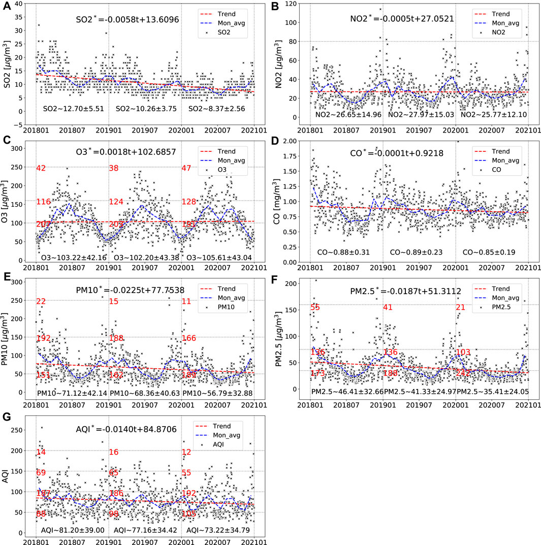
FIGURE 2. Time series of air-pollutant concentrations and AQI in Taizhou from 2018 to 2020: (A) SO2, (B) NO2, (C) O3, (D) CO, (E) PM10, (F) PM2.5, and (G) AQI. The scatter points show the daily data, the blue dashed lines are the monthly averages, and the red dashed lines are trend lines. Unitary linear regression models for each air pollutant are given at the top of each plot, and the mean and standard deviation for each year are shown at the bottom. The horizontal dotted lines show the thresholds of air-pollutant concentrations for the different levels of pollution. The numbers below the horizontal dotted lines show the number of days in each year that exceeded these pollution thresholds.
The results in Figures 1, 2 show that there is significant seasonal variation in both the number of pediatric respiratory outpatients and the air-pollutant concentrations. The inference is drawn that there is a certain correlation between them, and a quantitative assessment of this is now presented.
3.2 Possible factors affecting the number of pediatric respiratory outpatients
Figure 3 presents the detrended monthly time series of air-pollutant concentrations and the number of pediatric respiratory outpatients. The monthly data is used here because there is often a lag of a few days between a heavy air-pollution event and patients visiting the respiratory department. We use these data to explore the basic mechanism of how air-pollution-related factors affecting the pediatric respiratory diseases. The results demonstrate that the main air pollutants—NO2, CO, O3, PM2.5, and PM10—have significant correlations with the numbers of outpatients, with detrended Pearson correlation coefficients exceeding 0.35 (passing the 95% significance test). It also shows that the trends in the air-pollutant concentrations, aside from O3, are highly consistent with the outpatient visits; an increasing (decreasing) number of pediatric respiratory outpatients is seen with an increasing (decreasing) concentration of air pollutants. This indicates that the pediatric respiratory diseases are highly related to the air-pollutant factors, at least in statistics. A stratified analyse is further given as follows to confirm the point.
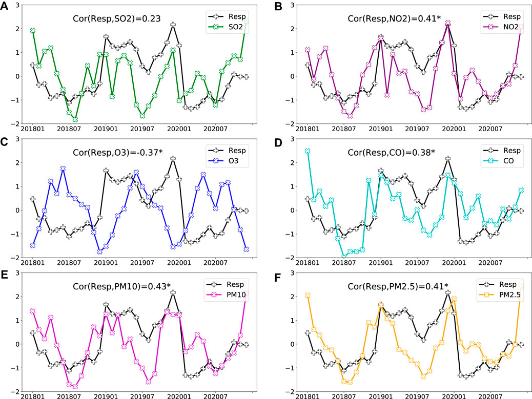
FIGURE 3. Normalized time series of detrended monthly air-pollutant concentrations (A) SO2, (B) NO2, (C) O3, (D) CO, (E) PM10, and (F) PM2.5, as well as the number of detrended pediatric respiratory outpatients from 2018 to 2020. The detrended Pearson correlation coefficients between the air-pollutant concentrations and the number of outpatients are listed at the top; the symbol * indicates that the correlation passes the 95% significance test.
The impacts of the seasons, the level of air pollution, and the type of primary pollutant on the clinic visits are presented in Figure 4. These histograms show that all three of these factors have significant effects on the incidence of pediatric respiratory diseases. Figures 4A–D show that the daily number of clinic visits in winter is almost twice that in the summer, which quantitatively demonstrates that there is remarkable seasonal variation. The comparisons in the levels of air pollution in Figures 4E–H show that the daily clinic visits gradually increase with increasing AQI level (i.e., with worse air quality). The daily number of pediatric respiratory outpatients increased from 47 in AQI I to 69 in AQI IV, which indicates that the air quality can significantly affect the incidence of pediatric respiratory disease. The results in Figures 4I–L show that the type of primary pollutant is another factor affecting the daily numbers of clinic visits. The excessive emission of PM2.5 and PM10 can lead to a notable increase in the number of pediatric respiratory outpatients. Conversely, the O3 concentration has a negative correlation with clinic visits. One of the reasons for this is that ozone-related pollution usually occurs in summer when the concentration of PM is at a low level.
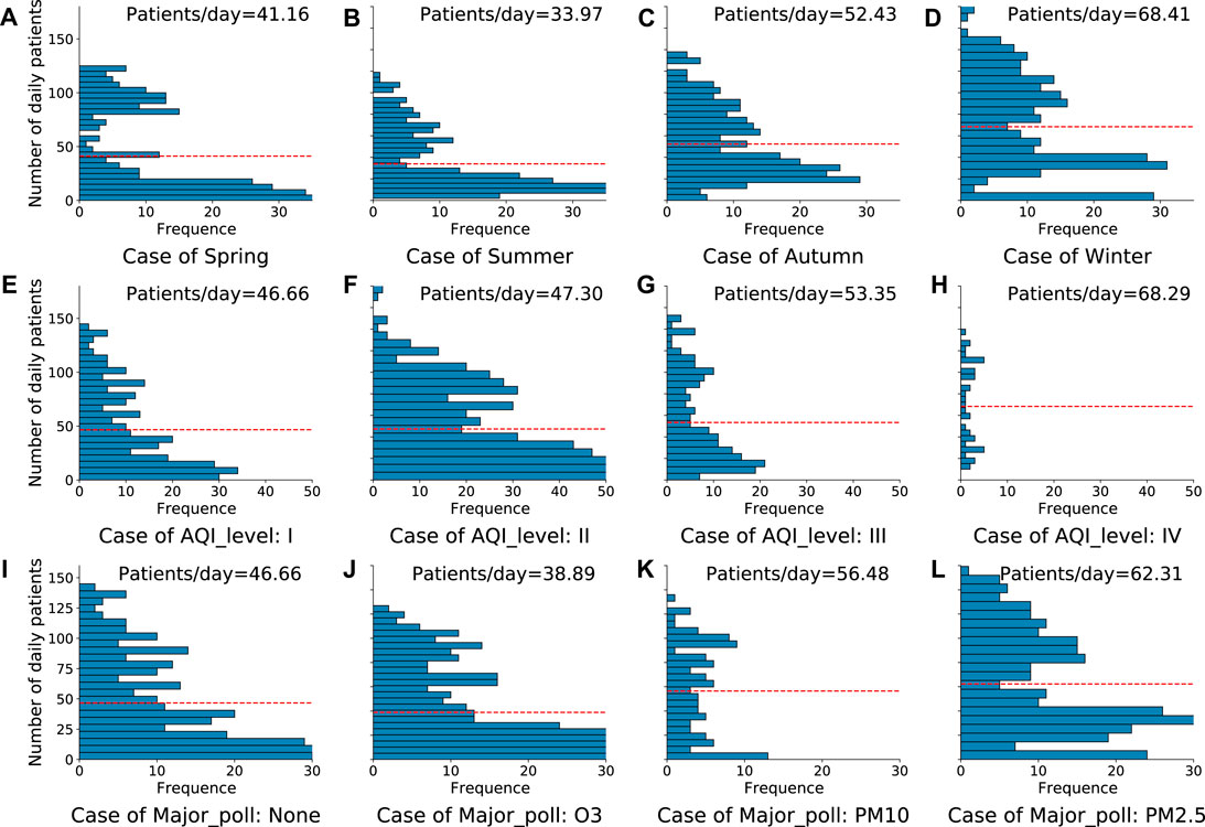
FIGURE 4. Frequency histograms of the total numbers of pediatric respiratory outpatients from 2018 to 2020 in different cases: (A–D) different seasons, (E–H) different levels of air pollution, and (I–L) different types of primary pollutant. The red dashed lines show the daily averages of the numbers of outpatients in each case.
3.3 ML regression models of air pollutants and pediatric respiratory outpatients
A number of ML methods were used to explore the statistical relationships among the air-pollutant concentrations and the numbers of pediatric respiratory outpatients. A monthly average was performed on the raw daily data to show the long-term impact. As noted in Section 2.1, the candidate predictors cover the concentrations of major air pollutants, the AQI, the level of air pollution, the type of primary pollutant, and temporal information. The log-transformed number of outpatients was used as the predictand. Hence, the regression model can be written as:
where Resp is the number of monthly clinic visits, ML () is the ML model, AQI_level is the level of air pollution, Major_pollutant is the type of primary pollutant and Month is the index of month.
Figure 5 presents the results of the simulation of the clinic visits by using ML models. The corresponding scores, root mean square error (RMSE), and correlation coefficient (CC) are listed at the top. These results show that all the ML models are able to capture the trend of the clinic visits and turning points. However, an underestimate is also seen in simulating the number of outpatients in 2019. Results in terms of RMSE and CC show that the non-linear models significantly outperform the linear ones. The RMSE values of the linear models, i.e., linear regression, ridge regression, and Huber regression, are greater than 30 persons/day, and their correlation coefficients are less than 0.6. The non-linear models, especially the RF, show superior performance, with RMSE values of less than 20 persons/day and CC values greater than 0.85.
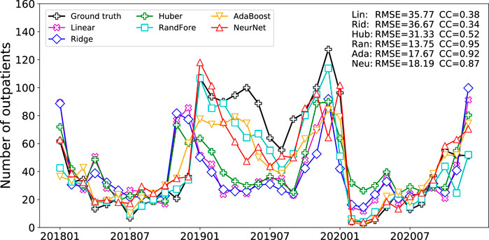
FIGURE 5. Monthly numbers of pediatric respiratory outpatients simulated by different ML models. The evaluation metrics, RMSE and CC, are given at the top.
It is noted that the purpose of this study was not to establish a high-quality prediction model for the number of pediatric respiratory outpatients but to explore the potential impact of the air pollutants on this number. The next section details the results of the application of a number of XAI methods to understanding the regression models built by the best-performing model, the RF.
3.4 Explanations of the RF model
The feature importance for the RF model, as obtained using the PFI method, is plotted in Figure 6. This shows that the AQI, the O3 concentration, and the month index are the three most important factors correlating with clinic visits. As noted earlier, the PFI method evaluates the global impact of each feature on the model prediction. However, it can only assess a single feature at a time, and it cannot show whether the impact is positive or negative. Hence, Figure 7 further presents an analysis of the contributions of O3 and PM10 using the PDP method.
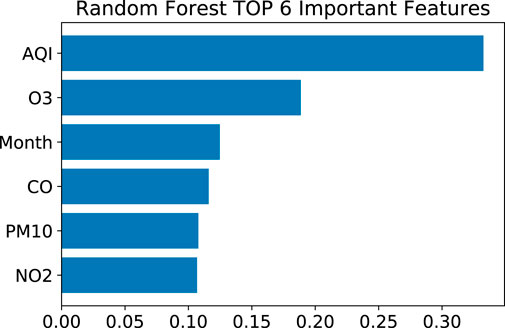
FIGURE 6. Feature importance for the trained RF model obtained using the PFI method.
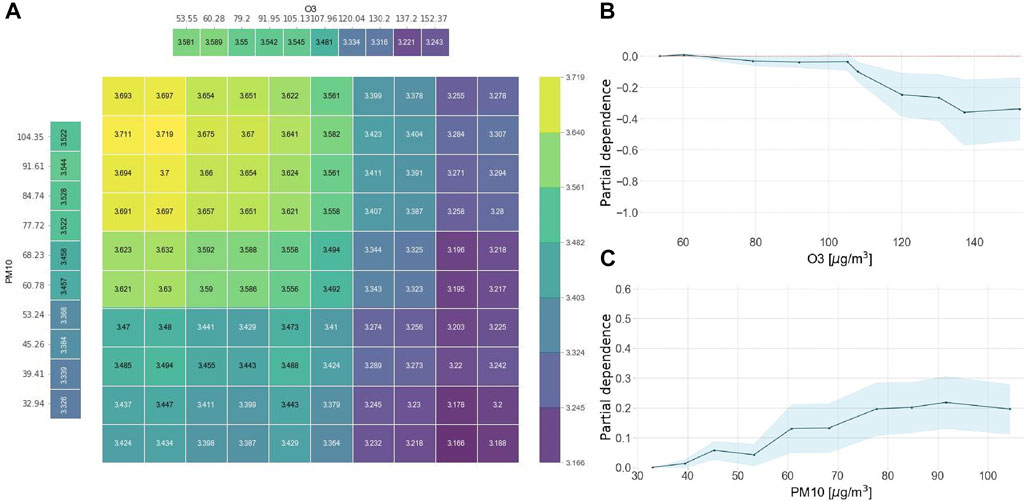
FIGURE 7. Feature importance of the O3 and PM10 concentrations for the trained RF model using a PDP. (A) Heat map showing the synergistic impact of O3 and PM10 on the number of outpatients, where the legend is the number of outpatients after the logarithm; PDPs showing the impacts of (B) O3 and (C) PM10.
Figure 7A shows how O3 and PM10 synergistically affect the number of clinic visits. The values in the heat map are the logarithm of the clinic visits, in which the warm (cold) tones indicate more (fewer) clinic visits. The impact of PM10 is given in the bar on the left side. An increasing number of clinic visits is seen from bottom to top as the concentration of PM10 increases. Similarly, the impact of O3 is presented at the top: an increase in the O3 concentration is correlated with a decrease in clinic visits. The heat map shows the joint impact of the O3 and PM10 concentrations on the number of pediatric respiratory outpatients. This indicates that increasing PM10 concentration and decreasing O3 concentration correlate with increasing clinic visits. The partial dependences of O3 and PM10 are respectively given in Figures 7B, C. These plots show that with increasing O3 concentration—especially when it exceeds 100 μg/m3—a clear decrease in the number of clinic visits is seen. The results for PM10 show that increasing PM10 concentration is correlated with a rapid increase in the number of clinic visits. It’s noted that the feature importance only gives the contribution of the factors on the model simulation in statistics. The underlying mechanism requires further experiments. Here, the contribution of PM10 is clear as pointed out in the WHO reports (World Health Organization, 2021; World Health Organization, 2022), while that of O3 is likely a statistical correlation. Nevertheless, the O3 concentration is an important indicator of respiratory disease in the view of feature importance.
The feature importance was further assessed using the SHAP method for the trained RF model, as shown in Figure 8. The colored scatter plot in Figure 8A shows the SHAP values of different features; the larger the SHAP value, the more important the feature for the model prediction. The color of each scatter point indicates the value of each feature. Taking AQI as an example, higher SHAP values for AQI values are generally positive, which indicates that AQI has a significant positive impact on the model results. Conversely, the SHAP values of higher O3 values are negative, which indicates a negative impact. Among the pollutants, NO2, CO, PM2.5, and PM10 show a promoting impact on clinic visits. Our results are in line with previous research (Yin et al., 2011; Shen et al., 2017; Song et al., 2018). Particulate matter can penetrate deep into the lungs and exposure to NO2 can irritate the respiratory tract, where both can further lead to respiratory symptoms. Figure 8B presents the feature importance as obtained using SHAP. The overall results are consistent with that assessed by the PFI method, which indicates that the interpretations of both of these XAI methods are credible.

FIGURE 8. SHAP feature importance for the trained RF model. (A) SHAP values of each feature; (B) mean of absolute SHAP values of each feature.
Local explanations of a given sample by SHAP and LIME are presented in Figure 9. The selected case happens in December 2019, which has the most clinic visits in a single month. Figure 9A shows the impacts of different predictors on the predictand with the SHAP method. A red (blue) arrow to the right (left) indicates that a factor has a positive (negative) contribution to the model to generate a high-value (low-value) prediction. The length of each arrow shows the degree of the contribution. The feature values are listed at the bottom, and the model prediction (after logarithm) is given in bold on the axis. In this case, almost all the predictors contribute to generating a high-value prediction, especially the joint effects of O3, NO2, and PM10. Figure 9B shows the assessment given by the LIME method. Similar to the results of SHAP, LIME shows that most of the predictors have positive contributions, except the AQI_level being a slightly inhibitory factor. Moreover, LIME can provide additional explanations using binary trees. For instance, the concentration of O3 in this case is 60.23 μg/m3 (see in Figure 9A), which is less the threshold 80.3 μg/m3 and causes the model to predict a higher value. The result is consistent with the PDP analysis in Figure 7B, which indicates that the model explanations given by LIME are reliable and easy to understand. It further assists the decision-making and the selection of important factors.

FIGURE 9. Case study of feature importance for the trained RF model with (A) SHAP and (B) LIME.
4 Conclusion and discussion
4.1 Conclusion
In this study, air pollution was found to be a major factor correlating with the incidence of pediatric respiratory diseases. Multiple ML models were used to explore the relationships between the air-pollutant concentrations and the numbers of pediatric respiratory outpatients in Taizhou, China. Different XAI methods were applied to explain the constructed model and analyze the feature importance. The main conclusions are as follows.
1. There is a significant seasonal variation in the number of clinic visits for pediatric respiratory diseases, and the peak value happens in the winter. Seasonal variation is seen in the concentrations of air pollutants. The concentrations of NO2, CO, PM2.5, and PM10 are higher in the winter, while that of O3 is higher in the summer. Among the air pollutants, NO2, CO, O3, PM2.5, and PM10 are significantly correlated with the numbers of clinic visits, with Pearson correlation coefficients greater than 0.35. Furthermore, comparisons between groups showed that the seasons, the level of air pollution, and the type of primary pollutant significantly affected the incidence of respiratory diseases in children. The concentration of PM was found to be the most important factor.
2. ML models are capable of well simulating the monthly clinic visits. The RMSE and CC results show that the non-linear models significantly outperform the linear ones. Among them, RF served as the best-performing model.
3. Four different XAI methods—PFI, PDP, SHAP, and LIME—were used for the explanation of the best-performing model, RF. The results showed that AQI, O3, PM, and the month were the four most important features. Among the air pollutants, increases in the concentrations of NO2, CO, PM2.5, and PM10 were correlated with increases in clinic visits. A case study in December 2019 showed that the SHAP and LIME methods are credible and easy to understand for local explanations of the RF model.
4.2 Discussion
The incidence of pediatric respiratory diseases is affected by a variety of factors, and air pollution is certainly one of the major causes. For instance, PM10 can penetrate deep in the lungs and PM2.5 can even enter the bloodstream, both leading to the respiratory symptoms (World Health Organization, 2021). Exposure to NO2 can irritate airways and aggravate respiratory diseases (World Health Organization, 2022). In this study, this incidence is characterized as the number of pediatric patients visiting the respiratory department of a single hospital in Taizhou. Comprehensive collection of clinic-visit information could further help to improve the reliability of the model. The purpose of the study was to explore the potential impact of air-pollutant concentrations on the incidence of pediatric respiratory diseases using ML models and XAI methods. Here, the monthly data was used which helped to abstract a clear and basic pattern of how air-pollution-related factors affecting the pediatric respiratory diseases. However, the small datasets could cause the over-fitting issue when training the ML models. Hence, interpretable ML models that prove still efficient for small datasets were adopted in this study, i.e. Adaboost and random forest. With this preliminary exploration, a prediction model for daily clinic visits will be investigated in future studies, where sufficient daily data can be used for training and validation. Furthermore, more factors should be taken into account aside from the air pollutants. The meteorological data, i.e. temperature and relative humidity (moisture), are commonly used to adjust the effects of weather on hospital outpatients (Song et al., 2018). The time lags between the air-pollution events and the patients visiting the hospital should also be included as additional factors.
Data availability statement
The raw data supporting the conclusion of this article will be made available by the authors, without undue reservation.
Author contributions
The study was conceived by YJ and YW. YJ and YZ contributed to the model development and maintained the code. YJ, TP, and LJ wrote the original draft. All authors reviewed and edited the manuscript. XZ supervised the entire project.
Funding
The work was jointly funded by the National Key Research and Development Program of China (Grant Nos. 2018YFC1507305, 2018YFC1507200, and 2017YFC1502000).
Conflict of interest
The authors declare that the research was conducted in the absence of any commercial or financial relationships that could be construed as a potential conflict of interest.
Publisher’s note
All claims expressed in this article are solely those of the authors and do not necessarily represent those of their affiliated organizations, or those of the publisher, the editors and the reviewers. Any product that may be evaluated in this article, or claim that may be made by its manufacturer, is not guaranteed or endorsed by the publisher.
References
Badue, C., Guidolini, R., Carneiro, R. V., Azevedo, P., Cardoso, V. B., Forechi, A., et al. (2021). Self-driving cars: A survey. Expert Syst. Appl. 165, 113816. doi:10.1016/j.eswa.2020.113816
Bojarski, M., Del Testa, D., Dworakowski, D., Firner, B., Flepp, B., Goyal, P., et al. (2016). End to end learning for self-driving cars. arXiv preprint arXiv:1604.07316.
Dominici, F., McDermott, A., Zeger, S. L., and Samet, J. M. (2002). On the use of generalized additive models in time-series studies of air pollution and health. Am. J. Epidemiol. 156, 193–203. doi:10.1093/aje/kwf062
Freeman, B. S., Taylor, G., Gharabaghi, B., and Thé, J. (2018). Forecasting air quality time series using deep learning. J. Air Waste Manag. Assoc. 68, 866–886. doi:10.1080/10962247.2018.1459956
Freund, Y., and Schapire, R. E. (1997). A decision-theoretic generalization of on-line learning and an application to boosting. J. Comput. Syst. Sci. 55, 119–139. doi:10.1006/jcss.1997.1504
Friedman, J. H. (2001). Greedy function approximation: A gradient boosting machine. Ann. Stat. 29, 1189–1232. doi:10.1214/aos/1013203451
Geiss, A., Silva, S. J., and Hardin, J. C. (2022). Downscaling atmospheric chemistry simulations with physically consistent deep learning. Geosci. Model. Dev. 15, 6677–6694. doi:10.5194/gmd-15-6677-2022
Gu, H., Yan, W., Elahi, E., and Cao, Y. (2020). Air pollution risks human mental health: An implication of two-stages least squares estimation of interaction effects. Environ. Sci. Pollut. Res. 27, 2036–2043. doi:10.1007/s11356-019-06612-x
Guo, Y., Barnett, A. G., Zhang, Y., Tong, S., Yu, W., and Pan, X. (2010). The short-term effect of air pollution on cardiovascular mortality in Tianjin, China: Comparison of time series and case–crossover analyses. Sci. Total. Environ. 409, 300–306. doi:10.1016/j.scitotenv.2010.10.013
Harrou, F., Dairi, A., Sun, Y., and Kadri, F. (2018). Detecting abnormal ozone measurements with a deep learning-based strategy. IEEE Sensors J. 18, 7222–7232. doi:10.1109/jsen.2018.2852001
Hesamian, M. H., Jia, W., He, X., and Kennedy, P. (2019). Deep learning techniques for medical image segmentation: Achievements and challenges. J. Digit. Imaging 32, 582–596. doi:10.1007/s10278-019-00227-x
Hoerl, A. E., and Kennard, R. W. (1970). Ridge regression: Applications to nonorthogonal problems. Technometrics 12, 69–82. doi:10.1080/00401706.1970.10488635
Hu, G., Yang, Y., Yi, D., Kittler, J., Christmas, W., Li, S. Z., et al. (2015). “When face recognition meets with deep learning: An evaluation of convolutional neural networks for face recognition,” in Proceedings of the IEEE International Conference on Computer Vision Workshops (Santiago, Chile: IEEE), 142–150. doi:10.1109/ICCVW.2015.58
Huber, P. J. (1973). Robust regression: Asymptotics, conjectures and Monte Carlo. Ann. Stat. 1, 799–821. doi:10.1214/aos/1176342503
Islam, M. S., Chaussalet, T. J., and Koizumi, N. (2017). Towards a threshold climate for emergency lower respiratory hospital admissions. Environ. Res. 153, 41–47. doi:10.1016/j.envres.2016.11.011
Kan, H., Chen, R., and Tong, S. (2012). Ambient air pollution, climate change, and population health in China. Environ. Int. 42, 10–19. doi:10.1016/j.envint.2011.03.003
Khaniabadi, Y. O., Goudarzi, G., Daryanoosh, S. M., Borgini, A., Tittarelli, A., and De Marco, A. (2017). Exposure to PM10, NO2, and O3 and impacts on human health. Environ. Sci. Pollut. Res. 24, 2781–2789. doi:10.1007/s11356-016-8038-6
Kleinert, F., Leufen, L. H., Lupascu, A., Butler, T., and Schultz, M. G. (2022). Representing chemical history in ozone time-series predictions–a model experiment study building on the MLAir (v1.5) deep learning framework. Geosci. Model. Dev. Discuss. 15, 8913–8930. doi:10.5194/gmd-15-8913-2022
Li, Y., Xiao, C., Li, J., Tang, J., Geng, X., Cui, L., et al. (2018). Association between air pollution and upper respiratory tract infection in hospital outpatients aged 0–14 years in hefei, China: A time series study. Public Health 156, 92–100. doi:10.1016/j.puhe.2017.12.006
Litjens, G., Kooi, T., Bejnordi, B. E., Setio, A. A. A., Ciompi, F., Ghafoorian, M., et al. (2017). A survey on deep learning in medical image analysis. Med. Image Anal. 42, 60–88. doi:10.1016/j.media.2017.07.005
Lundberg, S. M., and Lee, S. I. (2017). A unified approach to interpreting model predictions. Adv. Neural Inf. Process. Syst. 30, 4768. doi:10.5555/3295222.3295230
MacIntyre, E. A., Gehring, U., Mölter, A., Fuertes, E., Klümper, C., Krämer, U., et al. (2014). Air pollution and respiratory infections during early childhood: An analysis of 10 European birth cohorts within the ESCAPE Project. Environ. Health Perspect. 122, 107–113. doi:10.1289/ehp.1306755
McGovern, A., Elmore, K. L., Gagne, D. J., Haupt, S. E., Karstens, C. D., Lagerquist, R., et al. (2017). Using artificial intelligence to improve real-time decision-making for high-impact weather. Bull. Am. Meteorol. Soc. 98, 2073–2090. doi:10.1175/bams-d-16-0123.1
Parkhi, O. M., Vedaldi, A., and Zisserman, A. (2015). “Deep face recognition,” in Proceedings of the British Machine Vision Conference 2015 (Durham, DH1, UK: British Machine Vision Association), 1–12. doi:10.5244/C.29.41
Prüss-Üstün, A., Wolf, J., Corvalán, C., Bos, R., and Neira, M. (2016). Preventing disease through healthy environments: A global assessment of the burden of disease from environmental risks. Geneva, Switzerland: World Health Organization.
Qi, J., Ruan, Z., Qian, Z., Yin, P., Yang, Y., Acharya, B. K., et al. (2020). Potential gains in life expectancy by attaining daily ambient fine particulate matter pollution standards in mainland China: A modeling study based on nationwide data. PLoS Med. 17, e1003027. doi:10.1371/journal.pmed.1003027
Ravindra, K., Rattan, P., Mor, S., and Aggarwal, A. N. (2019). Generalized additive models: Building evidence of air pollution, climate change and human health. Environ. Int. 132, 104987. doi:10.1016/j.envint.2019.104987
Reichstein, M., Camps-Valls, G., Stevens, B., Jung, M., Denzler, J., Carvalhais, N., et al. (2019). Deep learning and process understanding for data-driven Earth system science. Nature 566, 195–204. doi:10.1038/s41586-019-0912-1
Ribeiro, M. T., Singh, S., and Guestrin, C. (2016). ““Why should I trust you?” explaining the predictions of any classifier,” in Proceedings of the 22nd ACM SIGKDD International Conference on Knowledge Discovery and Data Mining, 1135–1144. doi:10.1145/2939672.2939778
Ruckerl, R., Ibald-Mulli, A., Koenig, W., Schneider, A., Woelke, G., Cyrys, J., et al. (2006). Air pollution and markers of inflammation and coagulation in patients with coronary heart disease. Am. J. Respir. Crit. Care Med. 173, 432–441. doi:10.1164/rccm.200507-1123oc
Rumelhart, D. E., Hinton, G. E., and Williams, R. J. (1986). Learning representations by back-propagating errors. Nature 323, 533–536. doi:10.1038/323533a0
Sarnat, S. E., Raysoni, A. U., Li, W.-W., Holguin, F., Johnson, B. A., Luevano, S. F., et al. (2012). Air pollution and acute respiratory response in a panel of asthmatic children along the US–Mexico border. Environ. Health Perspect. 120, 437–444. doi:10.1289/ehp.1003169
Shahi, A. M., Omraninava, A., Goli, M., Soheilarezoomand, H. R., and Mirzaei, N. (2014). The effects of air pollution on cardiovascular and respiratory causes of emergency admission. Emergency 2, 107–114.
Shen, F., Ge, X., Hu, J., Nie, D., Tian, L., and Chen, M. (2017). Air pollution characteristics and health risks in Henan Province, China. Environ. Res. 156, 625–634. doi:10.1016/j.envres.2017.04.026
Song, J., Lu, M., Zheng, L., Liu, Y., Xu, P., Li, Y., et al. (2018). Acute effects of ambient air pollution on outpatient children with respiratory diseases in Shijiazhuang, China. BMC Pulm. Med. 18, 150. doi:10.1186/s12890-018-0716-3
Song, Y., Huang, B., He, Q., Chen, B., Wei, J., and Mahmood, R. (2019). Dynamic assessment of pm2. 5 exposure and health risk using remote sensing and geo-spatial big data. Environ. Pollut. 253, 288–296. doi:10.1016/j.envpol.2019.06.057
Terzi, Y., and Cengiz, M. (2009). Using of generalized additive model for model selection in multiple Poisson regression for air pollution data. Sci. Res. Essays 4, 867–871.
Wang, H. W., Li, X. B., Wang, D., Zhao, J., He, H. D., and Peng, Z. R. (2020). Regional prediction of ground-level ozone using a hybrid sequence-to-sequence deep learning approach. J. Clean. Prod. 253, 119841. doi:10.1016/j.jclepro.2019.119841
Wang, K. Y., and Chau, T. T. (2013). An association between air pollution and daily outpatient visits for respiratory disease in a heavy industry area. PLoS One 8, e75220. doi:10.1371/journal.pone.0075220
Wang, L., Liu, C., Meng, X., Niu, Y., Lin, Z., Liu, Y., et al. (2018a). Associations between short-term exposure to ambient sulfur dioxide and increased cause-specific mortality in 272 Chinese cities. Environ. Int. 117, 33–39. doi:10.1016/j.envint.2018.04.019
Wang, M., Zheng, S., Nie, Y., Weng, J., Cheng, N., Hu, X., et al. (2018b). Association between short-term exposure to air pollution and dyslipidemias among type 2 diabetic patients in northwest China: A population-based study. Int. J. Environ. Res. Public Health 15, 631. doi:10.3390/ijerph15040631
World Health Organization (2018a). 9 out of 10 people worldwide breathe polluted air, but more countries are taking action (news release). Geneva, Switzerland: World Health Organization. Available at: https://www.who.int/news-room/detail/02-05-2018-9-out-of-10-people-worldwide-breathe-polluted-air-but-more-countries-are-taking-action.
World Health Organization (2018b). Ambient (outdoor) air quality and health (news release). Geneva, Switzerland: World Health Organization. Available at: https://www.who.int/zh/news-room/fact-sheets/detail/ambient-(outdoor)-air-quality-and-health.
World Health Organization (2022). Billions of people still breathe unhealthy air: New who data (news release). Geneva, Switzerland: World Health Organization. Available at: https://www.who.int/news/item/04-04-2022-billions-of-people-still-breathe-unhealthy-air-new-who-data.
World Health Organization (2021). WHO global air quality guidelines: Particulate matter (PM2.5 and PM10), ozone, nitrogen dioxide, sulfur dioxide and carbon monoxide. Geneva, Switzerland: World Health Organization.
Xu, P., Chen, Y., and Ye, X. (2013). Haze, air pollution, and health in China. Lancet 382, 2067. doi:10.1016/s0140-6736(13)62693-8
Yin, Y., Chen, J., Duan, Y., Wei, H., Ji, R. X., Yu, J. L., et al. (2011). Correlation analysis between the PM2.5, PM10 which were taken in the hazy day and the number of outpatient about breathing sections, breathing sections of pediatrics in Shanghai. Environ. Sci. Chin. 32, 1894–1898.
Yu, M., and Liu, Q. (2021). Deep learning-based downscaling of tropospheric nitrogen dioxide using ground-level and satellite observations. Sci. Total. Environ. 773, 145145. doi:10.1016/j.scitotenv.2021.145145
Zhang, H., Wang, S., Hao, J., Wang, X., Wang, S., Chai, F., et al. (2016). Air pollution and control action in Beijing. J. Clean. Prod. 112, 1519–1527. doi:10.1016/j.jclepro.2015.04.092
Zhang, Z., Wang, J., Chen, L., Chen, X., Sun, G., Zhong, N., et al. (2014). Impact of haze and air pollution-related hazards on hospital admissions in Guangzhou, China. Environ. Sci. Pollut. Res. 21, 4236–4244. doi:10.1007/s11356-013-2374-6
Keywords: air pollutants, respiratory diseases in children, explainable artificial intelligence (XAI), feature importance analysis, Taizhou city
Citation: Ji Y, Zhi X, Wu Y, Zhang Y, Yang Y, Peng T and Ji L (2023) Regression analysis of air pollution and pediatric respiratory diseases based on interpretable machine learning. Front. Earth Sci. 11:1105140. doi: 10.3389/feart.2023.1105140
Received: 22 November 2022; Accepted: 14 February 2023;
Published: 01 March 2023.
Edited by:
Yi Li, Intel, United StatesReviewed by:
Haofei Yu, University of Central Florida, United StatesXueying Yu, Stanford University, United States
Xiao He, Shenzhen University, China
Ruizi Shi, Tsinghua University, China
Yimeng Song, Yale University, United States
Copyright © 2023 Ji, Zhi, Wu, Zhang, Yang, Peng and Ji. This is an open-access article distributed under the terms of the Creative Commons Attribution License (CC BY). The use, distribution or reproduction in other forums is permitted, provided the original author(s) and the copyright owner(s) are credited and that the original publication in this journal is cited, in accordance with accepted academic practice. No use, distribution or reproduction is permitted which does not comply with these terms.
*Correspondence: Xiefei Zhi, emhpQG51aXN0LmVkdS5jbg==