Reconstruction of seismic data based on SFISTA and curvelet transform

In seismic data processing, the reconstruction and interpolation of missing traces are essential tasks. To overcome the limitations of irregularly sampled seismic data, this paper proposes a seismic data interpolation method combining the smoothing fast iterative soft threshold algorithm (SFISTA) and the curvelet transform; this method uses the curvelet domain as the sparse domain. For comparison, the contourlet transform is used for different sparse domains, and the fast iterative shrinkage-thresholding algorithm (FISTA) is used for different optimization algorithms. Numerical modeling and real data show that the SFISTA method in the curvelet domain can give better reconstruction effects and higher reconstruction accuracy than those in the contourlet domain with the FISTA method; in addition, the SFISTA method in the curvelet domain can be used to reconstruct the missing traces of three-dimensional seismic data.

1 Introduction

In complex environments, seismic data reconstruction has great significance as a recovery technique. Under external disturbance, irregularly sampled seismic data will affect further geological data processing such as migration imaging and data interpretation. In order to obtain high-quality seismic data, interpolation reconstruction is needed to approximate the original data. In recent years, under the compressive sensing theory, seismic data reconstruction methods based on sparse constraints have become more and more popular. It mainly consists of the sparse transform, measurement matrix, and reconstruction algorithm. The sparse transforms that are often used include the Fourier transform (Zhang et al., 2013; Ciabarri et al., 2014), curvelet transform (Hennenfent et al., 2010; Liu et al., 2015; Zhang et al., 2017; Zhang et al., 2019; Tian and Qin, 2022), contourlet transform (Eslami and Radha, 2006), and seislet transform (Liu W et al., 2016). Because the curvelet transform undergoes multi-scale and multi-direction analysis and can perform the optimal local decomposition of seismic data (Yang et al., 2017), the curvelet transform is employed in this paper as a sparse transform, and the contourlet transform is also used in this paper for comparison analysis.

A classical sparse recovery problem usually requires minimizing the L₀ norm, which is NP-hard. The L₁ norm is the approximate of the L₀ norm, which is a convex function, and can be solved by the convex optimization algorithms or tools; so, the L₀ norm is replaced by the L₁ norm for simplicity and effectiveness. The iterative soft threshold algorithm (ISTA) shows great advantages (Daubechies et al., 2004; Mohsin et al., 2015) for a convex optimization algorithm. Gradually, a faster ISTA algorithm (FISTA) has been developed. FISTA is more suitable the synthesis approach to sparse recovery. And for the analysis approach to sparse recovery, Tan et al. (2014) proposed a monotone version of the fast iterative shrinkage-thresholding algorithm, which is the smoothing fast iterative soft threshold algorithm (SFISTA). In this paper, we introduce the SFISTA method-based curvelet transform to the seismic data interpolation reconstruction problem (Tan et al., 2014; Liu Y et al., 2016; Pokala and Seelamantula, 2020; Shen et al., 2020). The theory is given in section 2, and experimental results are given in section 3.

2 Theory

Assuming that the observed seismic data is $y$ and the downsampling matrix is $U$, the irregular missing seismic data can be modeled as follows:

$y=Ux+n,(1)$

where n is a randomly generated noise and $x$ is the original seismic data.

The interpolation problem can be expressed as follows:

$\underset{x}{\min }\frac{1}{2}‖y-{Ux‖}_2^2+\lambda {‖\mathrm{\Psi }x‖}_1,(2)$

where $‖{\bullet ‖}_2$ is the L₂ norm, $‖{\bullet ‖}_1$ is the L₁ norm, $\lambda$ is the regularization parameter, and $\mathrm{\Psi }$ is the analysis operator. Moreover, ${\mathrm{\Psi }}^{*}\mathrm{\Psi }=\mathrm{I}$, where ${\mathrm{\Psi }}^{*}$ denotes the adjoint of the operator $\mathrm{\Psi }$ and $\mathrm{I}$ is the identity matrix. The sparse transform can be expressed as $x=\mathrm{\Psi }\mathrm{\alpha }$, where $\mathrm{\Psi }$ is the transform operator and $\mathrm{\alpha }$ is the sparse coefficient. Let us denote the following equation:

$f\left(x\right)=\frac{1}{2}{‖Ux-y‖}_2^2,(3)$

where $f\left(x\right)$ is the smooth part.

$g\left(\mathrm{\Psi }x\right)=\mathrm{\lambda }{‖\mathrm{\Psi }x‖}_1,(4)$

where $g\left(\mathrm{\Psi }x\right)$ is the non-smooth part that needs to be replaced by the Moreau envelope with an approximately smooth form $g_{\mu }\left(\mathrm{\Psi }x\right)$, where $\mu$ is the smooth approximate parameter.

$\nabla g_{\mu }\left(\mathrm{\Psi }x\right)=\frac{1}{\mu }{\mathrm{\Psi }}^{*}\left(\mathrm{\Psi }x-T_{\lambda \mu }\left(\mathrm{\Psi }x\right)\right),(5)$

where $\nabla$ is the gradient and $T_{\lambda \mu }$ is the soft threshold operator; the threshold of $T_{\lambda \mu }$ is the multiplication of $\mathrm{\lambda }$ and $\mu$.

In this paper, the process of the smoothing fast iterative soft threshold algorithm (Shen et al., 2020) for optimization is expressed as follows:

$\nabla f\left({\widehat{x}}_k\right)=U^T\left(U{\widehat{x}}_k-y\right),(6)$

where $k$ is the number of iterations, and ${\widehat{x}}_0=x_0\mathrm{a}\mathrm{n}\mathrm{d}{t}_0=1$.

$\nabla g_{\mu }\left(\mathrm{\Psi }{x}_k\right)=\frac{1}{\mu }{\mathrm{\Psi }}^{*}\left(\mathrm{\Psi }{x}_k-T_{\lambda \mu }\left({\mathrm{\Psi }x}_k\right)\right).(7)$

The core iterations of the SFISTA are as follows:

$x_{k+1}={\widehat{x}}_k-\frac{1}{L}\left(\nabla f\left({\widehat{x}}_k\right)+\nabla g_{\mu }\left({\mathrm{\Psi }x}_k\right)\right),(8)$

where $L$ is the Lipschitz constant. At $0<\mathrm{\gamma }\le 1$, $L=1/\gamma$. Substituting (6) and (7) in (8), the aforementioned equation is equivalent to the following equation:

$x_{k+1}={\widehat{x}}_k-\frac{\gamma }{\mu }\left(x_k-{\mathrm{\Psi }}^{*}{T}_{\lambda \mu }\left(\mathrm{\Psi }{x}_k\right)\right)+\gamma U^T\left(y-U{\widehat{x}}_k\right),(9)$

where $\gamma$ is the iteration step size. $t_{k+1}$ is expressed as follows:

$t_{k+1}=\frac{1+\sqrt{1+4t_k^2}}{2}.(10)$

Then, we derive the following equation:

${\widehat{x}}_{k+1}=x_{k+1}+\frac{t_k-1}{t_{k+1}}\left(x_{k+1}-x_k\right).(11)$

The specific algorithm steps are as follows:

Algorithm 1. SFISTA for seismic data interpolation

Parameters: $\mathrm{\lambda }={10}^{-3},\mathrm{\mu }={10}^{-3}/\lambda =1,\mathrm{\gamma }=1/\left(1+1/\mu \right)$

Initialization: $x_0,{{\widehat{x}}_0,t}_0=1$

When not convergent, the following equations are used to calculate:

$x_{k+1}={\widehat{x}}_k-\frac{\gamma }{\mu }\left(x_k-{\mathrm{\Psi }}^{*}{T}_{\lambda \mu }\left(\mathrm{\Psi }{x}_k\right)\right)+\gamma U^T\left(y-U{\widehat{x}}_k\right)$

$t_{k+1}=\frac{1+\sqrt{1+4t_k^2}}{2}$

${\widehat{x}}_{k+1}=x_{k+1}+\frac{t_k-1}{t_{k+1}}\left(x_{k+1}-x_k\right)$

$\mathrm{R}\mathrm{L}\mathrm{N}\mathrm{E}=\frac{\parallel \widehat{x}-x{\parallel }_2}{\parallel x{\parallel }_2}$

end if $\mathrm{R}\mathrm{L}\mathrm{N}\mathrm{E}<{10}^{-6}$ or the maximum number of iterations is reached.

end

Output: $x$

Algorithm 2. FISTA for seismic data interpolation

Parameters: $\mathrm{\lambda }={10}^{-3},\mathrm{\gamma }=1$

Initialization: ${\alpha }_0,{{\widehat{\alpha }}_0,t}_0=1$

When not convergent, the following equations are used to calculate:

${\alpha }_{k+1}=T_{\gamma \lambda }\left(\gamma \mathrm{\Psi }{U}^T\left(y-U{\mathrm{\Psi }}^{*}{\alpha }_k\right)+{\widehat{\alpha }}_k\right)$

$t_{k+1}=\frac{1+\sqrt{1+4t_k^2}}{2}$

${\widehat{\alpha }}_{k+1}={\alpha }_{k+1}+\frac{t_k-1}{t_{k+1}}\left({\alpha }_{k+1}-{\alpha }_k\right)$

$\mathrm{R}\mathrm{L}\mathrm{N}\mathrm{E}=\frac{\parallel \widehat{\alpha }-\alpha {\parallel }_2}{\parallel \alpha {\parallel }_2}$

end if $\mathrm{R}\mathrm{L}\mathrm{N}\mathrm{E}<{10}^{-6}$ or the maximum number of iterations is reached.

end

Output: $\alpha$

3 Examples

In this section, we conduct numerical experiments with different seismic data to demonstrate the reconstruction performance of the SFISTA method in the curvelet domain. The algorithm performance is evaluated by interpolation results, the average amplitude spectrum, single-channel interpolation effect, reconstruction error, and signal-to-noise ratio. Numerical experiments are used to test the method. At last, the paper continues to test the 3D interpolation effect of the interpolation method of the proposed method. The experiments are conducted on a Millet computer running on the Windows 10 operating system and Inter Core m3-6Y30.

3.1 Synthetic examples

3.1.1 Seismic data interpolation in the contourlet domain

The regularization parameters of the FISTA and SFISTA methods are set to ${10}^{-3}.$ The step size of the FISTA is 1, and the step size of the SFISTA is set to 0.5 (Liu Y et al., 2016); the number of iterations is set as 500. The two-dimensional data tests have the same parameters.

Part data on the Marmousi2 model (Martin et al., 2006) are selected as test data; the data are shown in Figure 1A. Figure 1B shows the irregular data with 50% of the traces removed randomly, and this part’s records are padded with zeros. The sparse domain is the contourlet domain. Figures 1C,D are interpolation results of Figure 1B using FISTA and SFISTA methods based on the contourlet transform. Figures 1E,F show the reconstruction errors that correspond to the FISTA and SFISTA methods, in which the reconstruction residuals of the SFISTA method have smaller amplitude ranges than those of the FISTA method. It is obvious that the reconstruction method of SFISTA based on the contourlet transform is more effective.

FIGURE 1

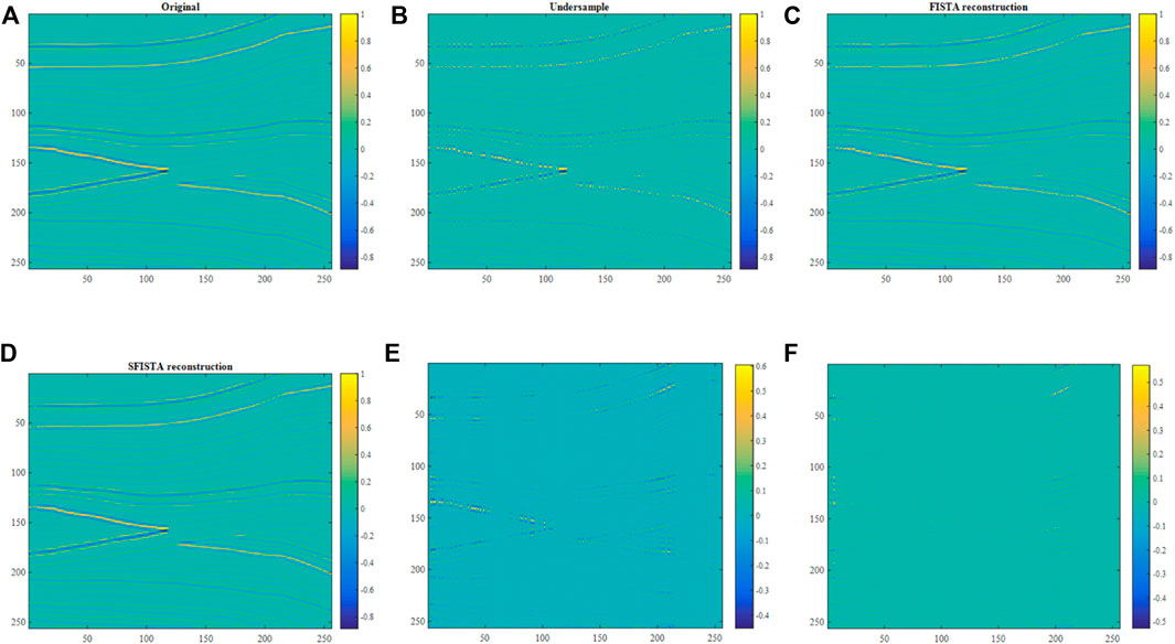
FIGURE 1. Reconstruction results of synthetic data in the contourlet domain. (A) Original data; (B) 50% of randomly missing data; (C) interpolated data obtained by the FISTA method; (D) interpolated data obtained by the SFISTA method; (E) reconstructed errors obtained by the FISTA method; (F) reconstructed errors obtained by the SFISTA method.

The performance of the proposed method in seismic data interpolation could be evaluated using different qualitative and quantitative analyzing tools. The reconstruction error is the general quantitative evaluation tool used in seismic data interpolation; the reconstruction error is defined to be $\sum \left|x-\widehat{x}\right|$, where $x$ denotes the original data and $\widehat{x}$ denotes the reconstructed seismic data. If the reconstruction error is smaller, the reconstructed seismic data will be closer to the original data. SNR is the signal-to-noise ratio, which is defined as $\mathrm{S}\mathrm{N}\mathrm{R}={101\mathrm{o}\mathrm{g}}_{10}\frac{{‖x‖}_2^2}{{‖x-\widehat{x}‖}_2^2}$. A higher SNR value means that the data have better reconstruction quality. The reconstruction error and signal-to-noise ratio are illustrated in Table 1. Table 1 shows that the SFISTA method has a smaller reconstruction error value and higher SNR. Compared to the two methods, the SFISTA method based on the contourlet transform has a lower reconstruction error and higher SNR, and therefore, the SFISTA method shows better performance.

TABLE 1

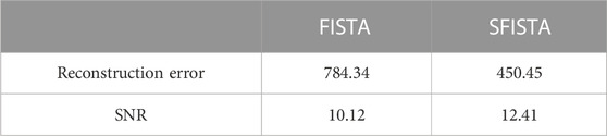
TABLE 1. Reconstruction error and SNR of different methods.

3.1.2 Seismic data interpolation in the curvelet domain

The part of the Marmousi2 model is shown in Figure 2A. Figure 2B shows the irregular data with 50% of the traces missing randomly. Figures 2C, D show interpolation effects using FISTA and SFISTA methods based on the curvelet transform. Figures 2E, F show the reconstruction errors that correspond to the FISTA and SFISTA methods, in which the reconstruction residuals of the SFISTA method have a smaller magnitude than those of the FISTA method. It is obvious that the reconstruction method of SFISTA in the curvelet domain is more effective.

FIGURE 2

FIGURE 2. Reconstruction results of synthetic data in the curvelet domain. (A) Original data; (B) 50% of randomly missing data; (C) interpolated data obtained by the FISTA method; (D) interpolated data obtained by the SFISTA method; (E) reconstructed errors obtained by the FISTA method; (F) reconstructed errors obtained by the SFISTA method.

Comparing Figures 1, 2, the SFISTA method in the curvelet domain has lower reconstruction errors when using the qualitative analyzing method. Comparing Tables 1, 2, the SFISTA method in the curvelet domain has lower reconstruction errors and higher SNR when using the quantitative analyzing method. The SFISTA method shows better performance when using the curvelet domain as the sparse domain.

TABLE 2

TABLE 2. Reconstruction error and SNR of different methods.

3.1.3 Coral reef model tests in the contourlet domain

The selected coral reef synthetic data are illustrated in Figure 3A. Figure 3B shows corrupted data with 50% of traces missing randomly. Figures 3C, D show interpolation effects using FISTA and SFISTA methods in the contourlet domain. Figures 3E, F show the reconstructed errors between the reconstruction and original data; Figure 3F shows a smaller reconstructed error. Table 3 shows the reconstruction error and SNR, which demonstrates the validity of the SFISTA method in the contourlet domain.

FIGURE 3

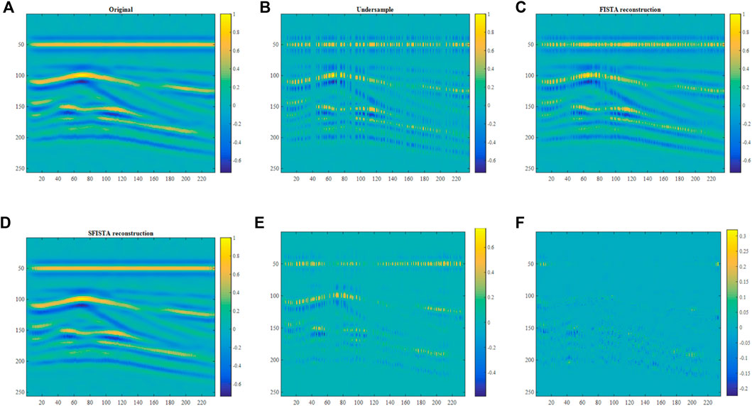
FIGURE 3. Reconstruction results of the coral reef model in the contourlet domain. (A) Original data; (B) 50% of randomly missing data; (C) interpolated data obtained by the FISTA method; (D) interpolated data obtained by the SFISTA method; (E) reconstructed errors obtained by the FISTA method; (F) reconstructed errors obtained by the SFISTA method.

TABLE 3

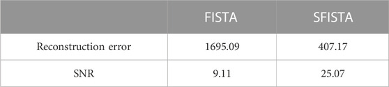
TABLE 3. Reconstruction error and SNR of different methods.

3.1.4 Coral reef model tests in the curvelet domain

The selected Coral reef synthetic data are tested in the curvelet domain; the original data are shown in Figure 4A. Figure 4B shows corrupted data with 50% of traces missing randomly. Figures 4C, D show interpolation results using FISTA and SFISTA methods in the curvelet domain. Figures 4E, F show the reconstructed errors between the reconstruction and original data; Figure 4F shows a smaller reconstructed error. Table 4 shows the reconstruction error and SNR, which demonstrates the validity of the proposed method.

FIGURE 4

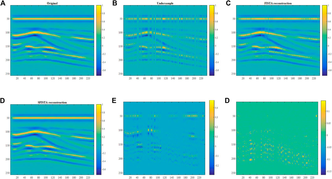
FIGURE 4. Reconstruction results of the coral reef model in the curvelet domain. (A) Original data; (B) 50% of randomly missing data; (C) interpolated data obtained by the FISTA method; (D) interpolated data obtained by the SFISTA method; (E) reconstructed errors obtained by the FISTA method; (F) reconstructed errors obtained by the SFISTA method.

TABLE 4

TABLE 4. Reconstruction error and SNR of different methods.

Comparing the detailed values in Tables 3, 4, the reconstruction performance of the SFISTA method in the curvelet domain is better than that in the contourlet domain.

3.2 Field examples

3.2.1 Seismic data interpolation in the contourlet domain

The field data are illustrated in Figure 5A. Figure 5B shows corrupted data with 50% of traces missing randomly. Figures 5C, D show interpolation effects using FISTA and SFISTA methods in the contourlet domain. By comparing the interpolation results of the ellipse regions, we learn that the reconstruction results of the SFISTA method in the contourlet domain are similar to the original data. Figures 5E, F show the reconstructed errors between the reconstruction and original data; Figure 5F shows a smaller reconstructed error. Table 5 shows the reconstruction error and SNR, which demonstrates the validity of the SFISTA method in the contourlet domain.

FIGURE 5

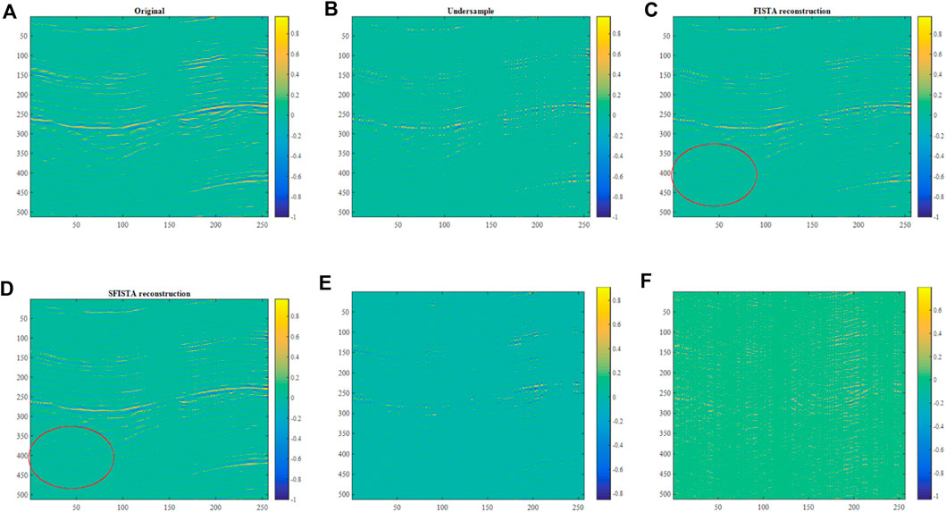
FIGURE 5. Reconstruction results of field data in the contourlet domain. (A) Original data; (B) 50% of randomly missing data; (C) interpolated data obtained by the FISTA method; (D) interpolated data obtained by the SFISTA method; (E) reconstructed errors obtained by the FISTA method; (F) reconstructed errors obtained by the SFISTA method.

TABLE 5

TABLE 5. Reconstruction error and SNR of different methods.

3.2.2 Seismic data interpolation in the curvelet domain

The field data are illustrated in Figure 6A. Figure 6B shows incomplete seismic data with 50% of traces missing randomly. Figures 6C, D show interpolation effects using FISTA and SFISTA methods in the curvelet domain. By comparing the interpolation results of the ellipse regions, we learn that the reconstruction data on the SFISTA method in the curvelet domain are similar to the original data. Figures 6E, F show the reconstructed errors between the reconstruction and original data; Figure 6F shows a smaller reconstructed error. Table 6 shows the reconstruction error and SNR results of the two algorithms in the curvelet domain. Comparing the two methods, SFISTA performs better with a lower error and higher SNR.

FIGURE 6

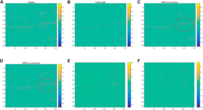
FIGURE 6. Reconstruction results of field data in the curvelet domain. (A) Original data; (B) 50% of randomly missing data; (C) interpolated data obtained by the FISTA method; (D) interpolated data obtained by the SFISTA method; (E) reconstructed errors obtained by the FISTA method; (F) reconstructed errors obtained by the SFISTA method.

TABLE 6

TABLE 6. Reconstruction error and SNR of different methods.

Figure 7A plots the interpolation single trace of the missing trace with zero values. In Figures 7, the black, pink, and blue lines correspond to the original data and those obtained by FISTA and SFISTA methods, respectively. Figure 7B shows the zoomed traces from the transparent gray window of Figure 7A. A detailed comparison reveals that the blue line is similar to the black line. We can, therefore, affirm that the proposed SFISTA method can better restore the significant features of the useful signal than the FISTA method.

FIGURE 7

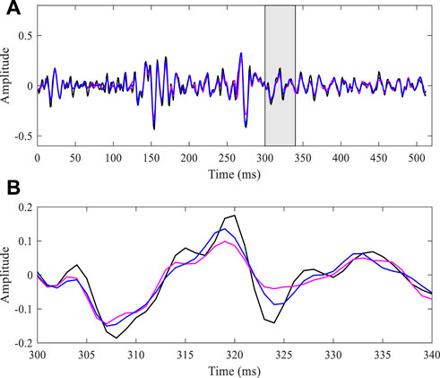
FIGURE 7. (A) Comparison of a missing single-trace amplitude interpolated with FISTA and SFISTA methods; (B) zoomed traces from the transparent gray window of (A).

Comparing the detailed values in Tables 5, 6, the SFISTA method in the curvelet domain is better than that in the contourlet domain.

The performance of these methods could be investigated more by comparing the average amplitude spectrum (Mafakheri et al., 2022). The average amplitude spectrum presents the original data and those obtained by FISTA and SFISTA methods, as shown in Figure 8 by the black, pink, and blue lines, respectively. The SFISTA method in the curvelet domain gives a closer spectrum to that of the original data, particularly in the range of 5–30 Hz. In this case, our method has better performance.

FIGURE 8

FIGURE 8. Average amplitude spectrum from original data, interpolated with FISTA and SFISTA methods.

3.2.3 Three-dimensional seismic data tests

The experimental results of three sets of 2D data show that SFISTA based on the curvelet transform shows good performance. Next, this method will be tested for 3D seismic data reconstruction. The 3D data (size: 64 × 64 × 64) are from the software package of MathGeo 2020 (https://gitee.com/sevenysw/MathGeo2020). The 3D discrete curvelet transform method comes from the reference of Ying et al. (2005).

The original data are shown in Figure 9A. Figure 9B shows corrupted data with 51% of the traces removed randomly; the iteration number of the FISTA and SFISTA methods is 1000. Figures 9C, D show the interpolation results using the FISTA and SFISTA methods in the curvelet domain. Figures 9E, F show reconstructed errors obtained by the FISTA and SFISTA methods. The quantitatively recovered reconstruction error and SNR are shown in Table 7; Table 7 illustrates that the SFISTA method is better than the FISTA method.

FIGURE 9

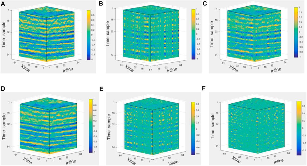
FIGURE 9. Reconstruction results of three-dimensional field data in the curvelet domain. (A) Original data; (B) 51% of randomly missing data; (C) interpolated data obtained by the FISTA method; (D) interpolated data obtained by the SFISTA method; (E) reconstructed errors obtained by the FISTA method; (F) reconstructed errors obtained by the SFISTA method.

TABLE 7

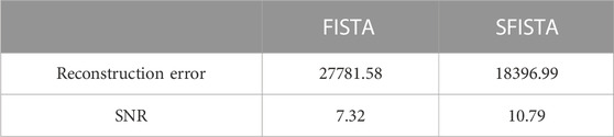
TABLE 7. Reconstruction error and SNR of different methods.

Figure 10A plots the interpolation single trace from Figures 9C, D. The black, pink, and blue lines represent the original data and those obtained by FISTA and SFISTA methods, respectively. Figure 10B shows the zoomed traces from the transparent gray window of Figure 10A. A detailed comparison reveals that the blue line is similar to the black line. We can, therefore, affirm that the proposed SFISTA method can better restore the significant features of the useful signal than the FISTA approach.

FIGURE 10

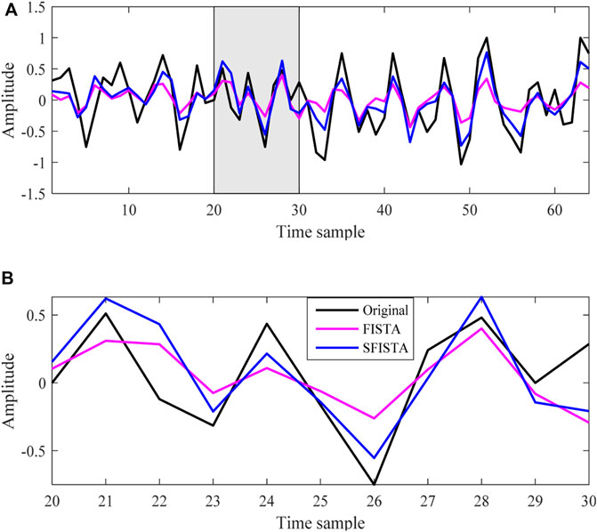
FIGURE 10. (A) Comparison of a missing single-trace amplitude interpolated with FISTA and SFISTA methods; (B) zoomed traces from the transparent gray window of (A).

The performance of these methods could be investigated more by comparing the average amplitude spectrum. The average amplitude spectrum of the original data and FISTA and SFISTA methods are shown in Figure 11 by the black, pink, and blue lines, respectively. Interestingly, in this case, the reconstruction data obtained by our method are very similar to the original data.

FIGURE 11

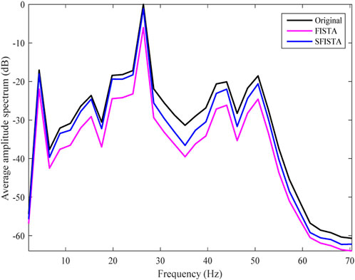
FIGURE 11. Average amplitude spectrum from original data, interpolated with FISTA and SFISTA methods.

4 Conclusion

In this paper, we proposed a new seismic data reconstruction method combining the curvelet transform and the SFISTA method. Comparing the results obtained when using the contourlet and curvelet domains as the sparse domain, it can be concluded that the optimization algorithm in the curvelet domain has better performance. In the same sparse domain, comparing the FISTA and SFISTA methods, it can be concluded that SFISTA shows better performance. The seismic data reconstruction effects of SFISTA based on the curvelet transform have been demonstrated by quantitative and qualitative comparisons with several sets of data. The proposed method can be used for 2D and 3D seismic data reconstruction.

Data availability statement

The original contributions presented in the study are included in the article/Supplementary Material; further inquiries can be directed to the corresponding author.

Author contributions

All authors listed have made a substantial, direct, and intellectual contribution to the work and approved it for publication.

Funding

This work was supported by the Yili Normal University Foundation under Grant 22XKZZ22, the Talent Position Project of Yili Normal University under Grant YSXSGG22006, and the National Natural Science Foundation of China under Grant 61761043.

Conflict of interest

The authors declare that the research was conducted in the absence of any commercial or financial relationships that could be construed as a potential conflict of interest.

Publisher’s note

All claims expressed in this article are solely those of the authors and do not necessarily represent those of their affiliated organizations, or those of the publisher, the editors, and the reviewers. Any product that may be evaluated in this article, or claim that may be made by its manufacturer, is not guaranteed or endorsed by the publisher.

References

Ciabarri, F., Mazzotti, A., Stucchi, E., and Bienati, N. (2014). Appraisal problem in the 3D least squares Fourier seismic data reconstruction. Geophys. Prospect. 63 (2), 296–314. doi:10.1111/1365-2478.12192

CrossRef Full Text | Google Scholar

Daubechies, I., Defrise, M., and Mol, C. D. (2004). An iterative thresholding algorithm for linear inverse problems with a sparsity constraint. Commun. Pure Appl. Math. 57 (11), 1413–1457. doi:10.1002/cpa.20042

CrossRef Full Text | Google Scholar

Eslami, R., and Radha, H. (2006). Translation-invariant contourlet transform and its application to image denoising. IEEE Trans. Image Process 15 (11), 3362–3374. doi:10.1109/tip.2006.881992

PubMed Abstract | CrossRef Full Text | Google Scholar

Hennenfent, G., Fenelon, L., and Herrmann, F. J. (2010). Nonequispaced curvelet transform for seismic data reconstruction: A sparsity-promoting approach. GEOPHYSICS 75 (6), 203–210. doi:10.1190/1.3494032

CrossRef Full Text | Google Scholar

Liu, W., Cao, S., Gan, S., Chen, Y., Zu, S., and Jin, Z. (2016). One-step slope estimation for dealiased seismic data reconstruction via iterative seislet thresholding. IEEE Geoscience Remote Sens. Lett. 13 (10), 1462–1466. doi:10.1109/lgrs.2016.2591939

CrossRef Full Text | Google Scholar

Liu, W., Cao, S., Li, G., and He, Y. (2015). Reconstruction of seismic data with missing traces based on local random sampling and curvelet transform. J. Appl. Geophys. 115, 129–139. doi:10.1016/j.jappgeo.2015.02.009

CrossRef Full Text | Google Scholar

Liu, Y., Zhan, Z., Cai, J.-F., Guo, D., Chen, Z., and Qu, X. (2016). Projected iterative soft-thresholding algorithm for tight frames in compressed sensing magnetic resonance imaging. IEEE Trans. Med. Imaging 35 (9), 2130–2140. doi:10.1109/TMI.2016.2550080

PubMed Abstract | CrossRef Full Text | Google Scholar

Mafakheri, J., Kahoo, A. R., Anvari, R., Mohammadi, M., Radad, M., and Monfared, M. S. (2022). Expand dimensional of seismic data and random noise attenuation using Low-Rank estimation. IEEE J. Sel. Top. Appl. Earth Observations Remote Sens. 15, 2773–2781. doi:10.1109/jstars.2022.3162763

CrossRef Full Text | Google Scholar

Martin, G. S., Wiley, R., and Marfurt, K. J. (2006). Marmousi2: An elastic upgrade for Marmousi. Lead. Edge 25 (2), 156–166. doi:10.1190/1.2172306

CrossRef Full Text | Google Scholar

Mohsin, Y. Q., Ongie, G., and Jacob, M. (2015). Iterative shrinkage algorithm for patch-smoothness regularized medical image recovery. IEEE Trans. Med. Imaging 34 (12), 2417–2428. doi:10.1109/tmi.2015.2398466

PubMed Abstract | CrossRef Full Text | Google Scholar

Pokala, P., and Seelamantula, C. (2020). “Accelerated weighted ℓ₁-minimization for MRI reconstruction under tight frames in complex domain,” in International Conference on Signal Processing and Communications (SPCOM), Bangalore, India, 19-24 July 2020. doi:10.1109/SPCOM50965.2020.9179611

CrossRef Full Text | Google Scholar

Shen, L., Chu, Z., Tan, L., Chen, D., and Ye, F. (2020). Improving the sound source identification performance of sparsity constrained deconvolution beamforming utilizing SFISTA. Shock Vib. 2020, 1–9. doi:10.1155/2020/1482812

CrossRef Full Text | Google Scholar

Tan, Z., Eldar, Y. C., Beck, A., and Nehorai, A. (2014). Smoothing and decomposition for analysis sparse recovery. IEEE Trans. Signal Process. 62 (7), 1762–1774. doi:10.1109/tsp.2014.2304932

CrossRef Full Text | Google Scholar

Tian, L., and Qin, S. (2022). “Seismic data interpolation by the projected iterative soft-threshold algorithm for tight frame,” in 2022 4th International Conference on Image Processing and Machine Vision (IPMV), Hong Kong China, March 25 - 27, 2022. doi:10.1145/3529446.3529460

CrossRef Full Text | Google Scholar

Yang, H., Long, Y., Lin, J., Zhang, F., and Chen, Z. (2017). A seismic interpolation and denoising method with curvelet transform matching filter. Acta Geophys. 65 (5), 1029–1042. doi:10.1007/s11600-017-0078-x

CrossRef Full Text | Google Scholar

Ying, L., Demanet, L., and Candes, E. (2005). 3D discrete curvelet transform. Proc. SPIE - Int. Soc. Opt. Eng. 50 (3), 351–361. doi:10.1117/12.616205

CrossRef Full Text | Google Scholar

Zhang, H., Chen, X.-H., and Wu, X.-M. (2013). Seismic data reconstruction based on CS and Fourier theory. Appl. Geophys. 10 (2), 170–180. doi:10.1007/s11770-013-0375-3

CrossRef Full Text | Google Scholar

Zhang, H., Chen, X.-H., and Zhang, L.-Y. (2017). 3D simultaneous seismic data reconstruction and noise suppression based on the curvelet transform. Appl. Geophys. 14 (1), 87–95. doi:10.1007/s11770-017-0607-z

CrossRef Full Text | Google Scholar

Zhang, H., Diao, S., Chen, W., Huang, G., Li, H., and Bai, M. (2019). Curvelet reconstruction of non-uniformly sampled seismic data using the linearized Bregman method. Geophys. Prospect. 67 (5), 1201–1218. doi:10.1111/1365-2478.12762

CrossRef Full Text | Google Scholar