Systematic diurnal bias of the CMA-MESO model in southern China: Characteristics and correction

Model error is an important source of numerical weather prediction (NWP) errors. Among model errors, the systematic diurnal bias plays an important role in high-resolution numerical weather prediction models. The main purpose of this study is to explore the characteristics of the systematic diurnal bias of a high-resolution NWP model in southern China and reduce the diurnal bias to improve the forecast results, hence providing a better background field for data assimilation. Based on the China Meteorological Administration Meso-scale (CMA-MESO) high-resolution NWP model, a 15-day sequential numerical weather prediction experiment was performed in southern China, and the forecast results were analyzed. A sequential bias correction scheme (SBCS) based on analysis increments was designed to reduce the systematic diurnal bias of the CMA-MESO model, and 15-day sequential comparative experiments were carried out. The analysis results showed that the CMA-MESO model has apparent systematic diurnal biases, and the characteristics differ among variables. A large diurnal bias was mainly found in the lower model layers, and it was concentrated in areas with a complex underlying surface for the horizontal distribution, such as the Qinghai-Tibet Plateau and South China Coast. The results based on the 15-day sequential experiment showed that the sequential bias correction scheme partly reduced the systematic diurnal biases of the CMA-MESO model. The mean biases of meridional wind, zonal wind, potential temperature, and water vapor mixing ratio were reduced by 45%, 35%, 20%, and 10%, respectively, and the root mean square errors (RMSEs) were reduced by approximately 5%. This study revealed the characteristics of the systematic diurnal bias of CMA-MESO model in southern China, which may be caused by the diurnal variation in the thermal and dynamic exchange on underlying surfaces. The effectiveness of the sequential bias correction scheme was also verified, and the results had good prospects for providing more reference information for high-resolution numerical prediction models and data assimilation.

1 Introduction

Numerical weather prediction (NWP) refers to a process in which the atmospheric governing equations are numerically integrated under given initial and boundary conditions to obtain the future atmospheric state (Xue and Chen, 2008). NWP isn’t only the basis of modern weather prediction but has also become an important research tool to determine the physical mechanisms and influencing factors of the occurrence and development of weather disasters. However, due to the non-linear and chaotic characteristics of the atmosphere, the initial errors and model errors of the NWP have a great impact on weather prediction (Lorenz, 1963; Bauer et al., 2015), which cause inaccurate forecast results.

Model errors can be classified as random errors and systematic bias (Dalcher and Kalnay, 1987; Murphy, 1988; Krishnamurti et al., 1999). The systematic bias mainly includes the mean and periodic bias such as associated with the annual cycle and the diurnal cycle (Bhargava et al., 2018), associated with the presence of short- or long-term bias, such as weather highs and lows, or the phase of El Niño (Danforth et al., 2007; Danforth and Kalnay, 2008a; Danforth and Kalnay, 2008b). Several studies have found that the systematic biases have some important influences on the forecast results. For example, the diurnal biases of atmospheric water vapor mixing ratio and the temperature play important roles in the energy budget and precipitation prediction for the NWP model (Dee and Todling, 2000; Dee, 2005; Svensson and Lindvall, 2015; Zhang et al., 2016; Bhargava et al., 2018; Patel et al., 2021). Dee and Todling (2000) analyzed the systematic bias in the NWP model and found that the systematic bias of the atmospheric water vapor mixing ratio plays an important role in the precipitation forecast of the model. The systematic bias of the 2-m temperature was found to show a strong diurnal cycle in the Global Forecast System (GFS) winter forecast results (Patel et al., 2021). In data assimilation, a background field that is assumed to be unbiased is needed to obtain the background error of the model and an accurate initial field. If the background field itself contains systematic bias, then the resulting initial field will also contain such bias (Dee and Arlindo, 1998; Dee, 2005; Zhang et al., 2016). This means that the systematic bias of an NWP model could also have a negative impact on its initial field through data assimilation (Bhargava et al., 2018). Therefore, it is necessary to identify the impacts of systematic bias on model forecasts and explore how it can be reduced.

In recent years, due to the increasing frequency of severe convective weather events and the demand for refined forecasting with a high spatial and temporal resolution, increasing attention has been given to high-resolution NWP models. It is worth noting that the systematic bias of short-term forecasts in high-resolution models often presents systematic diurnal bias (Bannister et al., 2019; Scaff et al., 2019; Chen et al., 2021). This bias plays an essential role in high-resolution models (Bhargava et al., 2018), and its influence cannot be ignored. (Faghih et al., 2022). Furthermore, the southern China is located in a subtropical and tropical region that is affected by tropical and temperate systems with complex underlying surfaces and often experiences heavy rains, tornados and other disastrous weather (Wu et al., 2011). Under such a complex background, if a high-resolution model directly performs a short-term forecast or data assimilation without considering the systematic diurnal bias, it may cause errors in the forecast and assimilation results. To solve these problems, some prior works proposed the systematic diurnal bias correction schemes based on Newtonian relaxation (nudging) method (Dee and Todling, 2000; Dee, 2005; Danforth et al., 2007), while some introduced the incremental analysis update (IAU) method (Zhang et al., 2016; Bhargava et al., 2018). For example, Dee and Todling (2000), Dee (2005) proposed an unbiased sequential analysis algorithm and corrected water vapor. And on top of Dee’s research, Zhang et al. (2016) proposed a correction algorithm to correct the diurnal bias of temperature, water vapor and wind. From the above studies, it can be found that the methods like IAU or Newtonian relaxation, which use analysis increments as constant forcings to gradually add them into the process of model integration (Bloom et al., 1996; Takacs et al., 2018), are effective means to correct the systematic bias.

However, most of the early studies focused on the correction of systematic bias in medium-term and long-term forecasts with low-resolution global models. Limited works were found for high-resolution short-term forecast in southern China. Therefore, this study aims at examining the characteristics of the systematic diurnal bias of the high-resolution model in southern China and correcting these biases. A 15-day sequential experiment was conducted based on the CMA-MESO model with a 3 km resolution in southern China, and the bias characteristics of the forecast results were analyzed. According to the analysis results a sequential bias correction scheme (SBCS) was designed based on the IAU approach, and 15-day sequential comparative experiments were carried out to test the SBCS performance. The results of this study are expected to be useful for reducing the systematic diurnal bias of the model, improving forecast results, and providing a better background field for data assimilation.

This paper is organized as follows. Section 2 introduces the model, analysis methods and experimental configuration. Section 3 analyzes the results, and Section 4 presents the conclusions.

2 Model, methods, and experimental configuration

2.1 Model configuration

A regional mesoscale model called the CMA-MESO that was developed by the China Meteorological Administration (CMA) Earth System Modeling and Prediction Centre (Chen et al., 2008) is used in this study. Table 1 shows the configurations of this model. The main features of the CMA-MESO include a fully compressible dynamic core with non-hydrostatic approximation, a semi-implicit and semi-Lagrangian scheme for time integration, and height-based terrain-following coordinates. The forecast region covers southern China and the South China Sea (16°–31.36°N, 96°–123.36°E) (shown in Figure 1), and the horizontal resolution of the model is 0.03° × 0.03° (3 km) with 51 vertical levels. The lateral boundary conditions and initial conditions of CMA-MESO are provided (directly downscaled) from the GFS developed by the National Center for Environmental Prediction (NCEP) and National Oceanic and Atmospheric Administration (NOAA).

TABLE 1

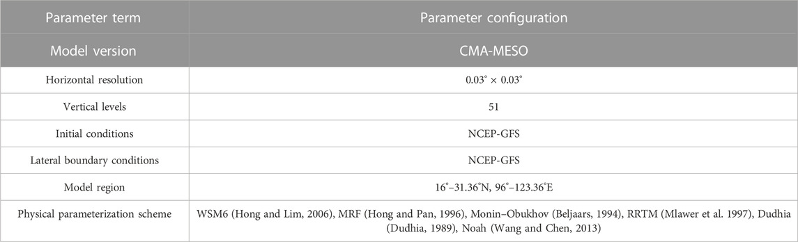
TABLE 1. Configuration of the CMA-MESO.

FIGURE 1

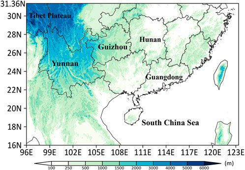
FIGURE 1. The model region and terrain height.

2.2 Bias analysis method and experimental configuration

In this study, the NCEP-GFS analysis field (hereafter referred to as the analysis data) is applied to evaluate the forecasts. The variables including the meridional wind (U), zonal wind (V), potential temperature (T), dimensionless pressure (Pi), and water vapor mixing ratio (Q) are derived from standard initialization process using the NCEP-GFS analysis data. It should be noted that all variables in this study are analyzed and corrected at the model layer.

Three evaluation metrics are applied in the following analysis, including the bias, the root-mean-square error (RMSE) and the diurnal bias amplitude (DBA):

$Bias=A_t-F_t(1)$

$RMSE=\sqrt{\frac{1}{n}{\displaystyle \sum }_{i=1}^n{\left(A_t-F_t\right)}^2}(2)$

$DBA=\left|{Bias}_{tmax}-{Bias}_{tmin}\right|(3)$

In the above equations, $A_t$ represents the analysis at time t; $F_t$ represents the forecast at time t; ${Bias}_{tmax}$ represents the maximum bias at different forecast times in a day; and ${Bias}_{tmin}$ represents the minimum bias at different forecast times in a day.

To analyze the characteristics of the bias in the CMA-MESO, 15-day sequential experiments are conducted (as shown in Table 2). The forecasts start at 0000, 0600, 1200, and 1800 UTC each day from June 1 to 15, 2022. The forecast lead time is 6 h.

TABLE 2

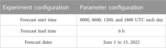
TABLE 2. Configuration of the analysis bias experiment.

2.3 Sequential bias correction scheme and experimental configuration

In this study, following Danforth et al. (2007), Danforth and Kalnay (2008a) and Bhargava et al. (2018), a sequential bias correction scheme (SBCS) based on the analysis increment was designed to correct the model diurnal bias. The 6-h analysis increment is obtained by subtracting the 6-h forecast result from the analysis data. This analysis increment can represent the systematic diurnal bias to a certain extent.

The detailed procedure for the SBCS is as follows:

Definitions: the model forecast value of a grid is defined as $N_f\left(t\right)$, which is calculated by $N_f\left(t\right)=M\left[t\right]$, where $t$ and $M\left[t\right]$ are the time and the process of the model forecast at the time, respectively. The analysis value of a grid is defined as $N_a\left(t\right)$, which is calculated by $N_a\left(t\right)=A\left[t\right]$, where $A\left[t\right]$ is the analysis value at time $t$. In this study, $N$ specifically refers to the variables to be corrected, namely, meridional wind (U), zonal wind (V), potential temperature (T), dimensionless pressure (Pi), and water vapor mixing ratio (Q).

(1) Derive the analysis increment $∆A\left(t\right)$ at time $t$ by subtracting the forecast value $N_f\left(t\right)$ from the analysis value $N_a\left(t\right)$ (as in Eq. 4.

(2) Calculate the average analysis increment $\overline{∆A}\left(t\right)$ by taking the mean value of the 6-h analysis increment $∆A\left(t\right)$ at different time t in the previous week Eq. 5. $n$ represents the sample number of $∆A\left(t\right)$ that is used to obtain the statistical average, and in this study, $n=7$.

(3) In the process of model integration, the corrected value $N_{f\left(mt\right)}$ of the variable $N_{f\_old\left(mt\right)}$ is calculated by Eq. 6, which is corrected stepwise at each step of integration. $\tau$ and $mt$ are the number of steps and each moment in the model integration, respectively.

$∆A\left(t\right)=N_a\left(t\right)-N_f\left(t\right)(4)$

$\overline{∆A}\left(t\right)=\frac{1}{n}{\displaystyle \sum }_{i=1}^n∆A\left(t\right)(5)$

$N_{f\left(mt\right)}=N_{f\_old\left(mt\right)}+\frac{\overline{∆A}\left(t\right)}{\tau }(6)$

Figure 2 gives the flowchart of the SBCS. As an example, to correct the systematic diurnal bias of the forecast at 0000 UTC on June 8, the average analysis increment $\overline{∆A}\left(t\right)$ is first derived from the forecast results of the previous week from 0000 UTC on June 1 to 0000 UTC on June 7. Then, the diurnal bias at 0000 UTC June 8 is corrected by subtracting $\overline{∆A}\left(t\right)$.

FIGURE 2

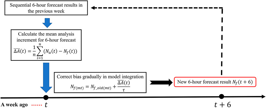
FIGURE 2. The flowchart of the SBCS.

In accordance with the above scheme, two groups of experiments were carried out from June 8 to 23, 2022. The CTL experiment was a control experiment without any bias correction scheme, and the BC experiment was a correction experiment using the SBCS (as shown in Table 3).

TABLE 3

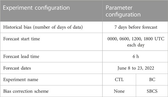
TABLE 3. Configuration of the analysis bias experiment.

3 Results

3.1 Diurnal bias characteristics

To analyze the characteristics of the bias in the CMA-MESO, 15-day sequential experiments are conducted. The systematic model bias can be detected by comparing forecasts against observations and calculating the regional averages of the mean biases in a relatively long time period (Dee and Todling, 2000). Figure 3 shows the evolution of the mean bias (dotted line) and RMSE (line) over time for the five variables. Because the Pi and Q values are too small, they are multiplied by 1,000 in this figure (the same treatment is hereafter noted in the figure title). Figure 3 shows that the mean bias of the model variables has diurnal characteristics. This diurnal characteristic of the mean bias presents some periodic diurnal changes with some irregular fluctuations in U, V, and Pi. However, it shows a continuous periodic diurnal cycle in T and Q, which presents obvious diurnal fluctuations. For example, the forecast mean bias of Q at 0000 UTC every day is always the lowest; then, it increases gradually at 0600 UTC, reaches the maximum mean bias at 1200 UTC, and finally decreases at 1800 UTC. This fluctuation obviously shows the diurnal characteristics. Other evolutions of mean bias, such as for U, also show diurnal characteristics, although noise exists. On the other hand, the RMSE also shows similar diurnal characteristics as the mean bias, which means that periodic diurnal bias exists in the CMA-MESO.

FIGURE 3

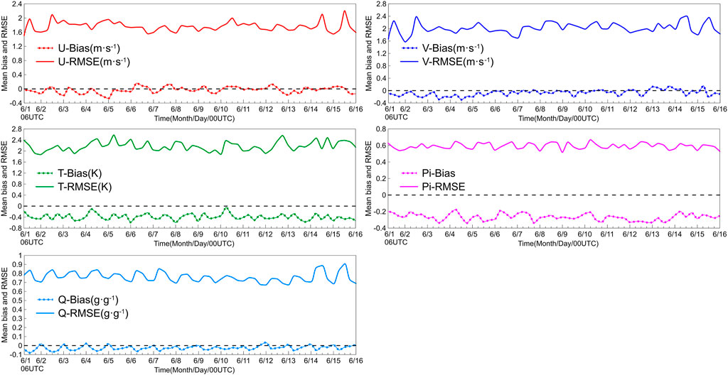
FIGURE 3. Evolution of the mean bias (dotted line) and RMSE (line) over time for U, V, T, Pi, and Q (Initialized at 0000, 0600, 1200, and 1800 UTC every day, with a forecast of 6 h, from 1 to 15 June 2022) (Pi and Q are multiplied by 1,000).

The power spectra of bias time series are another metric used to examine periodic characteristic (Zhang et al., 2016). Therefore, the 15-day forecast bias is used for Fourier spectrum analysis. Figure 4 shows the power spectra of (a) U, (b) T, (c) Pi and (d) Q in the forecast bias times series at different model layers from June 1 to 15, 2022 (the power spectra of V is similar to those of U, so they aren’t shown). The peaks are mostly concentrated in the spectrum within a 1-day period. This means that the most important periodic variation is the diurnal cycle for the mean bias of all variables. Among the four variables, the periodic variation in T and Q is dominated by the diurnal cycle, but the periodic variation in U and Pi is slightly more complicated. There are still serval secondary peaks, such as the 2-day and 4-day peaks, in the power spectra of U and Pi, which indicates periodic variation on a synoptic scale. On the other hand, the periodic variations in the low and middle model layers are still dominated by the diurnal cycle, and this characteristic is not obvious in the high model layer. This means that the mean bias of the diurnal cycle is mainly in the low and middle model layers.

FIGURE 4

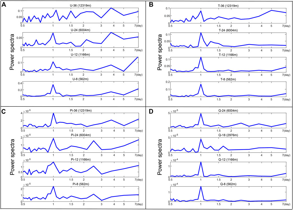
FIGURE 4. The power spectra of (A) U, (B) T, (C) Pi, and (D) Q in the forecast mean bias time series from June 1 to 15, 2022.

Figure 5 shows the spatial distribution of the vertical mean bias at different times (for example, the result at 0,600 UTC is the forecast result that started at 0000 UTC and forecasted 6-h). First, there are different spatial distributions of the vertical mean bias at different times, which means that the spatial distributions of the vertical mean bias have diurnal characteristics. For example, for U, the negative bias region is mainly on the Qinghai-Tibet Plateau and Yunnan-Guizhou Plateau, and the positive bias region is mainly on the South China Coast at 0600 UTC. At 1200 UTC, the negative bias region is mainly on the Qinghai-Tibet Plateau, Yunnan-Guizhou Plateau and in Guangdong Province, the maximum becomes larger, and the Qinghai-Tibet Plateau also shows some positive bias. At 1800 UTC, the area of negative bias increases, and there are only a small number of positive biases in Southeast Asia and the South China Sea. At 0000 UTC, the whole area is dominated by negative bias. Second, the spatial distribution of the vertical mean bias has some characteristics related to the underlying surface. For U and V, the large bias region is mainly on the Qinghai-Tibet Plateau and Yunnan-Guizhou Plateau, which have high altitudes, many mountains and a complex topography. For Pi and Q, the large bias region is mainly in the South China Coast and South China Sea, which have the ocean and coasts.

FIGURE 5

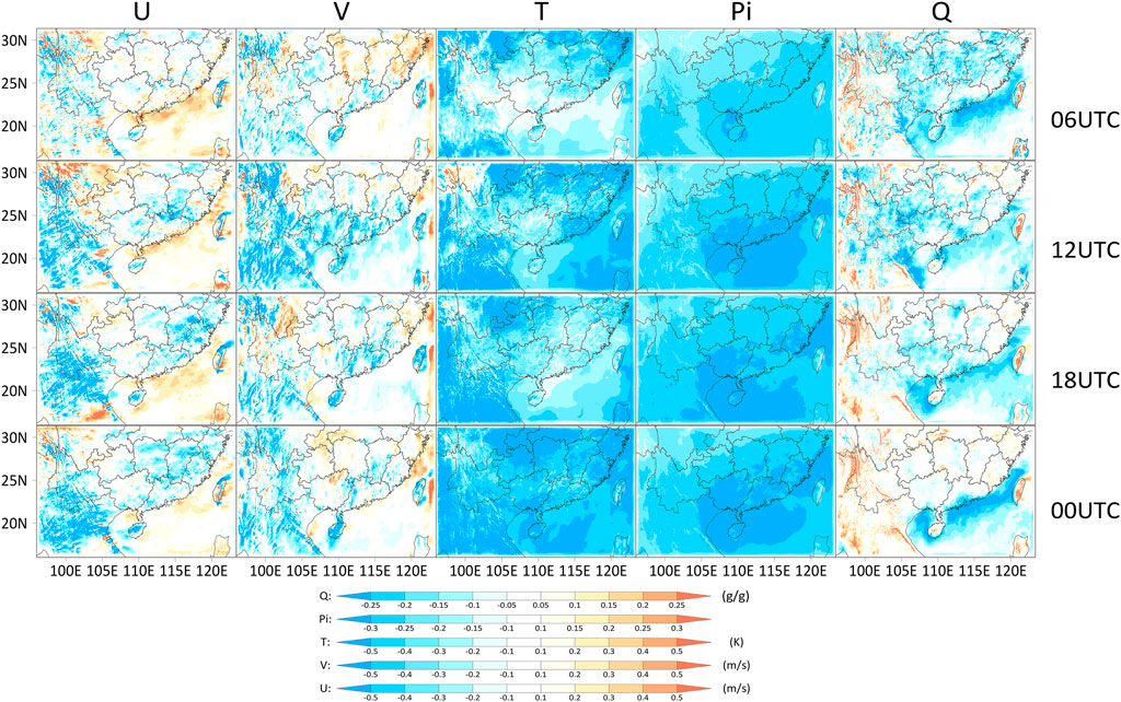
FIGURE 5. The spatial distribution of the vertical mean bias at different times (cool colors represent a negative bias and warm colors represent a positive bias) (Pi and Q are multiplied by 1,000).

To explore the impact of the underlying surface on the diurnal bias variation for the low model layers, an indicator called DBA is defined. The DBA is calculated by Eq. 3, and it can show the region with a large diurnal variation in the bias. Figure 6 shows the spatial distribution of DBA at layers 1, 13 and 18. From Figure 6, it can be seen that the region of large DBA is mainly concentrated on the Qinghai-Tibet Plateau, Yunnan-Guizhou Plateau, in Taiwan, and Southeast Asia; these areas are characterized by high altitudes, multiple mountains, and complex underlying surfaces. Especially for T, the temperature is easily affected by the radiation of the underlying surface. Therefore, the DBA value of T is large in 1-layer, and it shows an obvious relation between the underlying surface, as shown in Figure 6. However, in the 13-layer and 18-layer, the impact of the underlying surface gradually decreases with increasing altitude. This means that the diurnal bias may be directly affected by the diurnal variation in the thermal and dynamic exchange on underlying surfaces, and this influence will gradually decrease with increasing altitude.

FIGURE 6

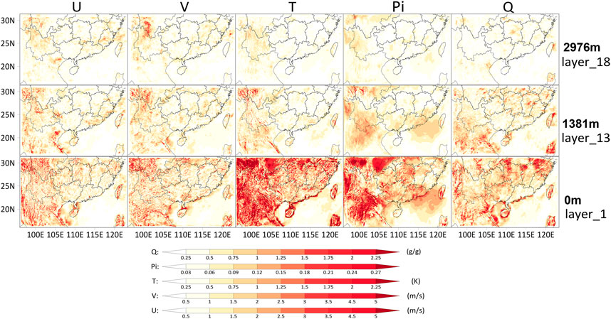
FIGURE 6. The spatial distribution of the DBA at 1, 13, and 18 model layers (Pi and Q are multiplied by 1,000).

Figure 7 is the vertical profile of the horizontal forecast mean bias and RMSE from June 1 to 15, 2022. First, the mean bias has an overall trend of large values in the lower and high model layers and small values in the middle model layers. Second, the vertical profile of the four start times presents a different distribution, especially for the lower layer. For example, the vertical profiles of U and V show clear diurnal characteristics. It can also be found that the amplitude of the diurnal bias is large in the lower layer but small in the middle and high layers. On the other hand, the vertical profile of the RMSE also presents a similar feature to that of mean bias. The results of the vertical profile verify the previous results. The lower layer is easily affected by changes in the underlying surface, and the systematic diurnal bias is mainly present in the lower model layer.

FIGURE 7

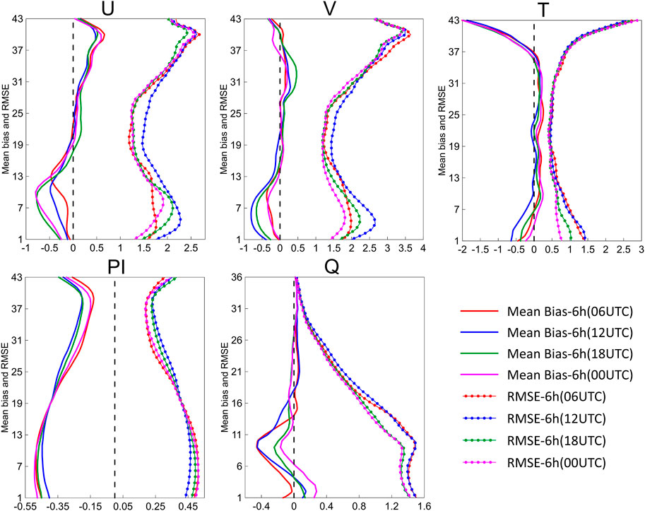
FIGURE 7. The vertical profiles of the horizontal mean bias and RMSE from June 1 to 15, 2022 (Pi and Q are multiplied by 1,000).

According to the above results, it can be found that the forecast mean bias and RMSE of CMA-MESO have some diurnal features. These diurnal biases are concentrated on plateaus and mountains and in oceans and lakes for the horizontal distribution and in the low model layer for the vertical distribution. This phenomenon may be mainly caused by the direct impact of the diurnal variation on the underlying surface.

3.2 Diurnal bias correction

From the above analysis, it can be seen that there are systematic diurnal biases in the CMA-MESO forecast results in southern China. To correct these biases in the model and improve the forecast results, the SBCS is designed, and two comparative experiments are carried out. One is the BC experiment using the SBCS, and the other is the CTL experiment without any bias correction scheme. According to the results, Figure 8 shows the evolution of the mean bias (dotted line) over time for some variables with important weather information at different model layers. In addition, in Figure 8, the 36-layer, 24-layer, 12-layer and 8-layer are selected to represent high layer, middle layer, middle-lower layer and lower layer in the model, respectively. The mean bias of U generally decreases in the high layer, middle layer and lower layer after using the SBCS (as shown in Figures 8A–C). Moreover, it is worth noting that the amplitude of the diurnal bias also decreases, especially in the lower layer (as shown in Figure 8C), which means that the systematic diurnal bias is reduced. For the Pi in the middle layer, which is often used to represent synoptic situations, the mean bias of the BC experiment is lower than that of the CTL experiment (as shown in Figure 8D). For T in the middle layer, the mean biases of the two experiments are similar (as shown in Figure 8E). However, in the lower layer, the mean bias of the BC experiment is lower than that of the CTL experiment, and the amplitude of the diurnal bias also decreases (as shown in Figure 8F). For Q in the middle-lower layer and lower layer, the mean biases of the BC experiment are lower than those of the CTL experiment, and the amplitude of the diurnal bias also decreases (as shown in Figures 8G, H). In general, the mean biases and the amplitude of the diurnal bias are partly reduced after correction with the SBCS scheme.

FIGURE 8

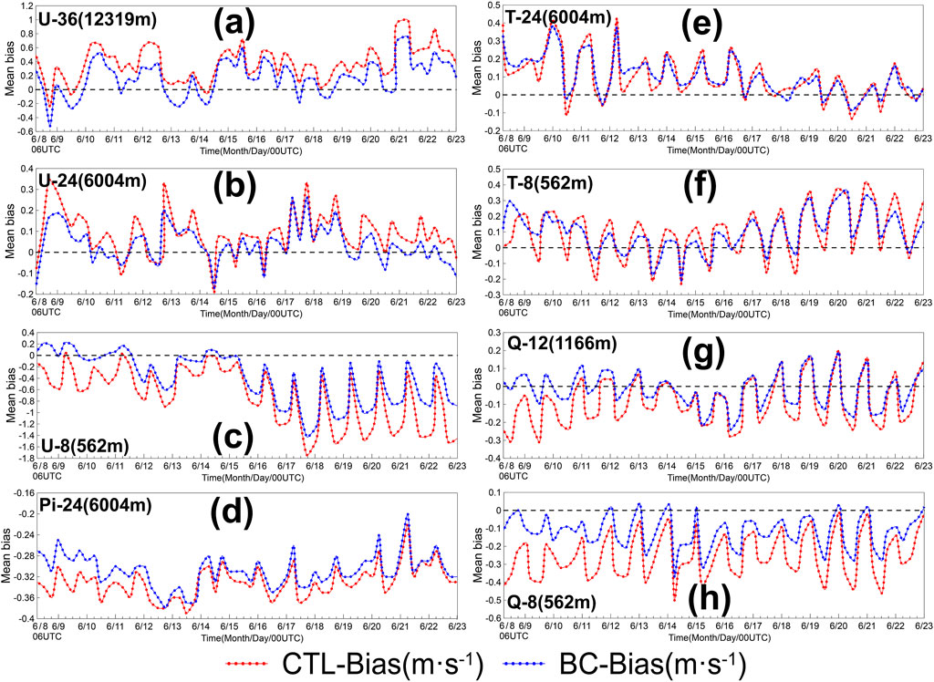
FIGURE 8. Evolution of the mean bias (dotted line) over time for the U, T, Pi, and Q values at different model layers. (A) U in 36-layer, (B) U in 24-layer, (C) U in 8-layer, (D) Pi in 24-layer, (E) T in 24-layer, (F) T in 8-layer, (G) Q in 12-layer, and (H) Q in 8-layer (initialized at 0000, 0600, 1200, and 1800 UTC every day, with a forecast of 6 h, from 8 to 23 June 2022) (Pi and Q are multiplied by 1,000).

Figure 9 shows the power spectra of (a) U, (b) T, (c) Pi and (d) Q in the forecast bias times series for the BC (blue line) and CTL (red line) experiments at different model layers from June 8 to 23, 2022 (the power spectra of V is similar to U, so they aren’t shown). The peak of the CTL experiment is still mostly concentrated in the spectrum within a 1-day period. However, the peak of the BC experiment within a 1-day period decreases at most layers. For some of these variables, such as the T at the high layer, the peak over a 1-day period even disappears. In addition, although the peak is decreased, diurnal fluctuation still exists for most of the variables. This means that the SBCS scheme can only partly reduce the systematic diurnal bias but cannot completely eliminate the influence of such bias on the model forecast results.

FIGURE 9

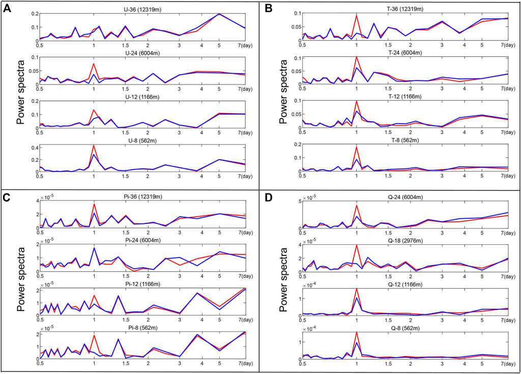
FIGURE 9. The power spectra of (A) U, (B) T, (C) Pi and (D) Q in the forecast mean bias time series for the BC (blue line) and CTL (red line) experiments at different model layers from June 8 to 23, 2022.

To determine if there is any change in the spatial distribution of the model bias after using the SBCS, Figure 10 shows the spatial distribution of the vertical mean bias at different times for the BC and CTL experiments. Figure 10A shows that the area and value of the U mean bias in the BC experiment are smaller than those in the CTL experiment in areas such as the Qinghai-Tibet Plateau, Yunnan-Guizhou Plateau and southeast region. Figures 10B–D also show similar the results as Figure 10A, the mean biases of the BC experiment are reduced, and the forecast results are improved. In addition, the improved regions are different. In detail, for the V, the improved region is concentrated in the South China Coast and on Qinghai-Tibet Plateau; for the T, the improved region is concentrated in the north and southeast; for the Pi, the improved region is concentrated in the South China Coast and South China Sea areas; and for the Q, the improved region is concentrated in the South China Coast and on Yunnan-Guizhou Plateau. In general, the improved region is closely related to the underlying surface, such as plateau, mountain, coast and ocean.

FIGURE 10

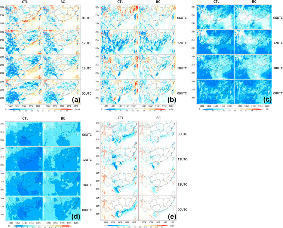
FIGURE 10. The spatial distribution of the vertical mean bias at different times for the BC and CTL experiments. (A) U, (B) V, (C) T, (D) Pi and (E) Q. (Pi and Q are multiplied by 1000).

As mentioned earlier, the diurnal bias is closely related to the underlying surface, and Figure 10 also shows an improvement in the BC experiment in regions with a complex underlying surface. What are the characteristics of the mean bias and RMSE at different vertical layers after using the SBCS? Figure 11 shows the vertical profiles of the horizontal mean bias (line) and RMSE (dotted line) for the BC (blue) and CTL (red) experiments. The mean bias of the BC experiment is generally smaller than that of the CTL experiment, which means that the forecast result of the BC is improved and the diurnal bias of the model is partly corrected. For U, V, T, and Q, the model bias of the BC experiment is obviously reduced in the high and lower layers, and there is little change in the middle layer. On the other hand, for the forecast results at different times, the correction effect at 1200 UTC and 1800 UTC is better than that at 0000 UTC and 0600 UTC. However, for Pi, this improvement is not apparent. The mean bias of the BC experiment decreases at 0000 UTC and 0600 UTC in the lower layers, and there is little change at other times in the high and middle layers. In general, it can be seen that the results of the BC experiment show lower mean bias and RMSE, especially for the lower model layers, which shows apparent improvement.

FIGURE 11

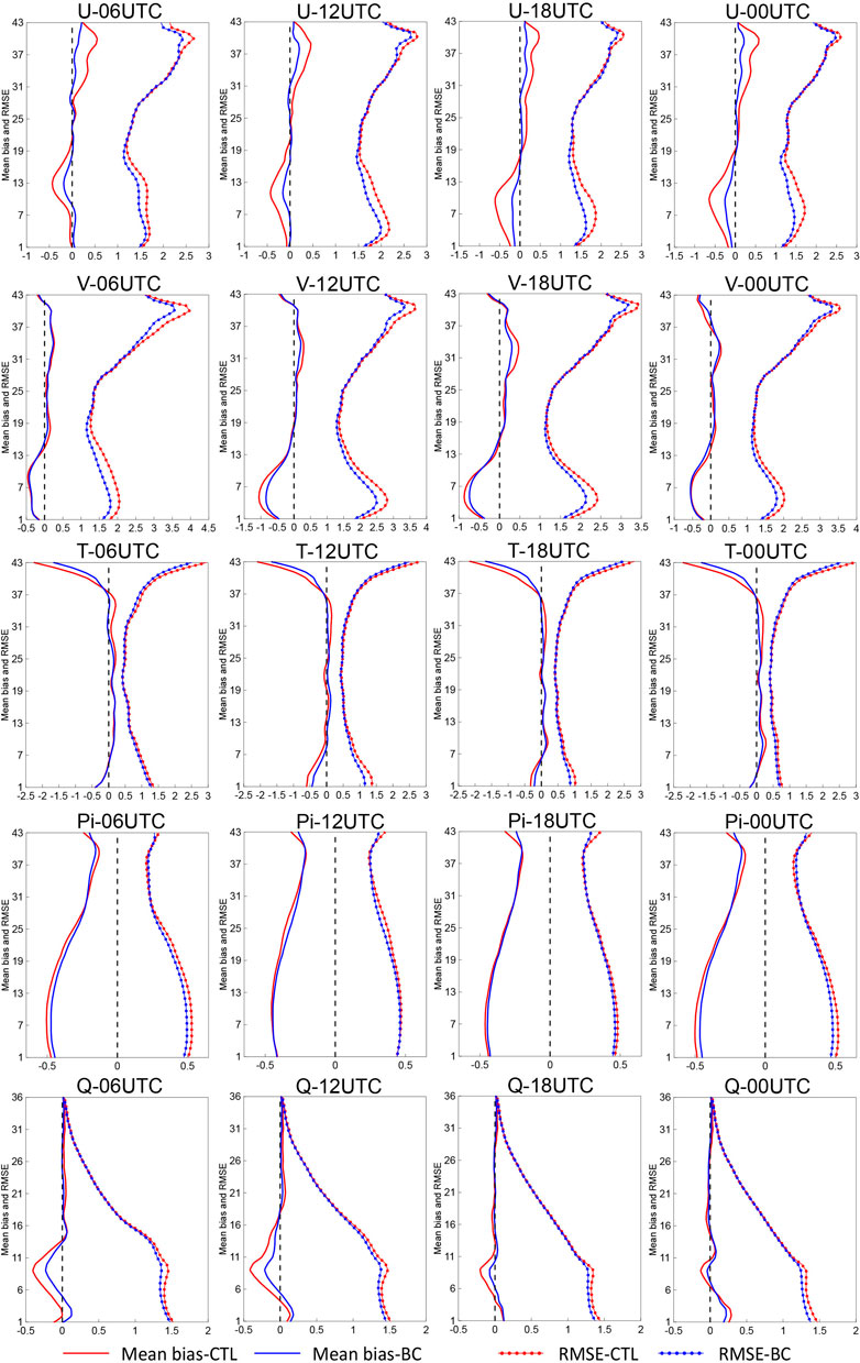
FIGURE 11. The vertical profiles of the horizontal mean bias and RMSE for the BC and CTL experiments (initialized at 0000, 0600, 1200, and 1800 UTC every day, with a forecast of 6 h, from 8 to 23 June 2022). (Pi and Q are multiplied by 1,000).

The improvement rate (IR, which is calculated by equation $IR=\frac{\left({\left|X\right.}_{CTL}|-\left|X_{BC}\right|\right)}{\left|X_{CTL}\right|}\times 100\%$, where $X$ represents the mean bias or RMSE) at different times is introduced to better show the improvement of the forecast results using the SCBS (as shown in Figure 12). Here, $X$ represents the mean bias or RMSE of all grids respectively. A positive IR represents a positive improvement, and a negative IR represents a worse performance. From the Figure 12, it is found that both the bias and RMSE show positive improvement in all variables at all times. Specifically, the IR (bias) of U at all times nearly exceeds 40%; the IR (bias) of T at all times nearly exceeds 20%; and the IR (bias) of Q at all times nearly exceeds 30%. The improvement of V and Pi is relatively small; the IR (bias) of V is only approximately 10%, and that of Pi is only approximately 5%. On the other hand, the IR (RMSE) is generally lower than the IR (bias), and those of U, V, T, Pi, and Q are approximately 10%, 7%, 8%, 5%, and 4%, respectively.

FIGURE 12

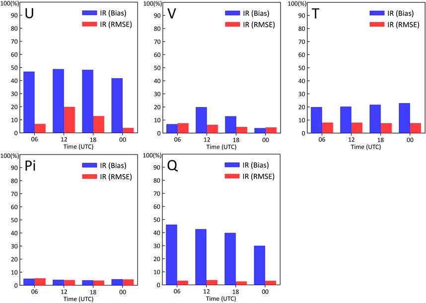
FIGURE 12. The improvement rate for the BC and CTL experiments at different times (blue bars indicate the improvement rate of the bias, and red bars indicate the improvement rate of the RMSE).

According to the above results, it is found that the mean bias and RMSE of the BC experiment using the SBCS are generally lower than those of the CTL experiment. Furthermore, the SBCS reduced the systematic diurnal bias and improved the forecast results in the CMA-MESO.

4 Summary and discussion

In this study, the bias characteristics of the 15-day sequential experiment results in southern China are analyzed based on the CMA-MESO high-resolution NWP model. According to the analysis results, the sequential bias correction scheme called the SBCS was designed to reduce systematic diurnal bias with using analysis increments in the CMA-MESO. Two sequential, 15-day comparative experiments are carried out, one using the SBCS and the other being a control treatment without any bias correction scheme.

The detailed procedures related to the SBCS within CMA-MESO are addressed in this paper. Specifically, the historical 6-h continuous forecast results of the week before the forecast time are used to obtain the analysis increments of each grid point through statistical averaging. Then, through model integration, the variable is corrected stepwise at each step of integration.

The preliminary results of the bias analysis show that the CMA-MESO has a systematic diurnal bias in southern China. The bias of each variable has different characteristics at different times of the day. Specifically, for the horizontal distribution, the systematic diurnal bias is mainly concentrated on the Qinghai-Tibet Plateau, Yunnan-Guizhou Plateau, South China Coast and in the South China Sea. These areas have complex underlying surfaces, such as plateaus, mountains, lakes, coasts and oceans. For the vertical distribution, the systematic diurnal bias is concentrated in the lower model layer, which is susceptible to the underlying surface. This phenomenon may be caused by the influence of the diurnal variation in the thermal and dynamic exchange on underlying surfaces. On the other hand, the preliminary results of bias correction show that the SBCS partly reduces systematic diurnal biases, and reduces the mean bias of the CMA-MESO 6-h forecast by 5%–50% and the RMSE by 4%–10%. This means that the SBCS reduces the systematic diurnal bias and improves the forecast results of the CMA-MESO in southern China.

This study shows the characteristics of systematic diurnal bias in southern China with the CMA-MESO high-resolution model and the positive correction effect of the SBCS. However, with in-depth research, there are still some problems and challenges that need to be overcome. First, in this study, the purpose of the SBCS is to improve both the model forecast results and the background field in data assimilation. However, we have not conducted an assimilation experiment using the corrected forecast results with the SBCS. This will be our next major research direction. Second, for the improvement of the forecast results with the SBCS, we have only carried out a 6-h forecast at present, without carrying out a longer-term (such as 24-h or 36-h) forecast experiment. More sensitive experiments are needed. In the future, we will further explore these problems.

Data availability statement

The raw data supporting the conclusions of this article will be made available by the authors, without undue reservation.

Author contributions

YC: Conceptualization, methodology, design and experiment, investigation, formal analysis, writing draft. LW: Methodology, funding acquisition, supervision, writing—review and editing. JL: Methodology, writing—review and editing. DX: Writing—review and editing. JC: Resources. BZ: Conceptualization, funding acquisition, supervision, writing—review and editing.

Funding

This work was supported by National Key R&D Program of China (Grant No. 2021YFC3000902), the National Natural Science Foundation of China (Grant No. U2142213), and the Guangdong Basic and Applied Basic Research Foundation (Grant No. 2020A1515110040).

Support for model computing resources was provided by the CMA Earth System Modeling and Prediction Centre. And the initial and boundary conditions for this work were provided by the CMA Earth System Modeling and Prediction Centre.

Conflict of interest

The authors declare that the research was conducted in the absence of any commercial or financial relationships that could be construed as a potential conflict of interest.

Publisher’s note

All claims expressed in this article are solely those of the authors and do not necessarily represent those of their affiliated organizations, or those of the publisher, the editors and the reviewers. Any product that may be evaluated in this article, or claim that may be made by its manufacturer, is not guaranteed or endorsed by the publisher.

References

Bannister, D., Orr, A., Jain, S. K., Holman, I. P., Momblanch, A., Phillips, T., et al. (2019). Bias correction of high-resolution regional climate model precipitation output gives the best estimates of precipitation in Himalayan catchments. J. Geophys. Res.-Atmos. 124, 14220–14239. doi:10.1029/2019JD030804

CrossRef Full Text | Google Scholar

Bauer, P., Thorpe, A., and Brunet, G. (2015). The quiet revolution of numerical weather prediction. Nature 525, 47–55. doi:10.1038/nature14956

PubMed Abstract | CrossRef Full Text | Google Scholar

Beljaars, A. C. M. (1994). The parametrization of surface fluxes in large-scale models under free convection. Quart. J. Roy. Meteor. Soc. 121, 255–270. doi:10.1002/qj.49712152203

CrossRef Full Text | Google Scholar

Bhargava, K., Kalnay, E., Carton, J. A., and Yang, F. (2018). Estimation of systematic errors in the GFS using analysis increments. J. Geophys. Res. Atmos. 123, 1626–1637. doi:10.1002/2017jd027423

CrossRef Full Text | Google Scholar

Bloom, S. C., Takacs, L. L., Sliva, A. M. D., and Ledvina, D. (1996). Data assimilation using incremental analysis updates. Mon. Wea. Rev. 124, 1256–1271. doi:10.1175/1520-0493(1996)124<1256:dauiau>2.0.co;2

CrossRef Full Text | Google Scholar

Chen, D. H., Xue, J. S., Yang, X. S., Zhang, H., Shen, X., Hu, J., et al. (2008). New generation of multiscale NWP system (GRAPES): General scientific design. Chin. Sci. Bull. 53, 3433–3445. doi:10.1007/s11434-008-0494-z

CrossRef Full Text | Google Scholar

Chen, Y. D., Fang, K. M., Chen, M., and Wang, H. L. (2021). Diurnally varying background error covariances estimated in RMAPS-ST and their impacts on operational implementations. Atmos. Res. 257, 105624. doi:10.1016/j.atmosres.2021.105624

CrossRef Full Text | Google Scholar

Dalcher, A., and Kalnay, E. (1987). Error growth and predictability in operational ECMWF forecasts. Tellus A 39A (5), 474–491. doi:10.3402/tellusa.v39i5.11774

CrossRef Full Text | Google Scholar

Danforth, C. M., and Kalnay, E. (2008b). Impact of online empirical model correction on nonlinear error growth. Geophys. Res. Lett. 35, L24805. doi:10.1029/2008gl036239

CrossRef Full Text | Google Scholar

Danforth, C. M., Kalnay, E., and Miyoshi, T. (2007). Estimating and correcting global weather model error. Mon. Weather Rev. 135, 281–299. doi:10.1175/mwr3289.1

CrossRef Full Text | Google Scholar

Danforth, C. M., and Kalnay, E. (2008a). Using singular value decomposition to parameterize state-dependent model errors. J. Atmos. Sci. 65, 1467–1478. doi:10.1175/2007jas2419.1

CrossRef Full Text | Google Scholar

Dee, D. P., and Arlindo, M. D. S. (1998). Data assimilation in the presence of forecast bias. Quart. J. Roy. Meteor. Soc. 124, 269–295. doi:10.1002/qj.49712454512

CrossRef Full Text | Google Scholar

Dee, D. P. (2005). Bias and data assimilation. Quart. J. Roy. Meteor. Soc. 131, 3323–3343. doi:10.1256/qj.05.137

CrossRef Full Text | Google Scholar

Dee, D. P., and Todling, R. (2000). Data assimilation in the presence of forecast bias: The GEOS moisture analysis. Mon. Wea. Rev. 128, 3268–3282. doi:10.1175/1520-0493(2000)128<3268:daitpo>2.0.co;2

CrossRef Full Text | Google Scholar

Dudhia, J. (1989). Numerical study of convection observed during the Winter Monsoon Experiment using a mesoscale two-dimensional model. J. Atmos. Sci 46, 3077–3107. doi:10.1175/1520-0469(1989)046,3077:NSOCOD.2.0.CO;2

CrossRef Full Text | Google Scholar

Faghih, M., Brissette, F., and Sabeti, P. (2022). Impact of correcting sub-daily climate model biases for hydrological studies. Hydrology Earth Syst. Sci. 26, 1545–1563. doi:10.5194/hess-26-1545-2022

CrossRef Full Text | Google Scholar

Hong, S.-Y., and Pan, H.-L. (1996). Nonlocal boundary layer vertical diffusion in a medium-range forecast model. Mon. Weather. Rev. 124, 2322–2339. doi:10.1175/1520-0493(1996)124,2322:NBLVDI.2.0.CO;2

CrossRef Full Text | Google Scholar

Hong, S.-Y., and Lim, J.-O. J. (2006). The WRF single-moment 6-class microphysics scheme (WSM6). J. Korean Meteor. Soc. 42 (2), 129–151.

Google Scholar

Krishnamurti, T. N., Kishtawal, C. M., Timothy, T., Bachiochi, D. R., Zhang, Z., Williford, C. E., et al. (1999). Improved weather and seasonal climate forecasts from multimodel super ensemble. Science 285 (5433), 1548–1550. doi:10.1126/science.285.5433.1548

PubMed Abstract | CrossRef Full Text | Google Scholar

Lorenz, E. N. (1963). Deterministic nonperiodic flow. J. Atmos. Sci. 20 (2), 130–141. doi:10.1175/1520-0469(1963)020<0130:dnf>2.0.co;2

CrossRef Full Text | Google Scholar

Mlawer, E. J., Taubman, S. J., Brown, P. D., Iacono, M. J., and Clough, S. A. (1997). Radiative transfer for inhomogeneous atmospheres: RRTM, a validated correlated-k model for the longwave. J. Geophys. Res. 102, 16663–16682. doi:10.1029/97JD00237

CrossRef Full Text | Google Scholar

Murphy, A. H. (1988). Skill scores based on the mean square error and their relationships to the correlation coefficient. Mon. Weather Rev. 116 (12), 2417–2424. doi:10.1175/1520-0493(1988)116<2417:ssbotm>2.0.co;2

CrossRef Full Text | Google Scholar

Patel, R. N., Yuter, S. E., Miller, M. A., Rhodes, S. R., Bain, L., and Peele, T. W. (2021). The diurnal cycle of winter season temperature errors in the operational Global Forecast System (GFS). Geophys. Res. Lett. 48, e2021GL095101. doi:10.1029/2021gl095101

CrossRef Full Text | Google Scholar

Scaff, L., Prein, A. F., Li, Y., Liu, C., Rasmussen, R., and Ikeda, K. (2019). Simulating the convective precipitation diurnal cycle in North America’s current and future climate. Clim. Dynam. 55, 369–382. doi:10.1007/s00382-019-04754-9

CrossRef Full Text | Google Scholar

Svensson, G., and Lindvall, J. (2015). Evaluation of near-surface variables and the vertical structure of the boundary layer in CMIP5 models. J. Clim. 28, 5233–5253. doi:10.1175/jcli-d-14-00596.1

CrossRef Full Text | Google Scholar

Takacs, L. L., Suárez, M. J., and Todling, R. (2018). The stability of incremental analysis update. Mon. Weather Rev. 146 (10), 3259–3275. doi:10.1175/mwr-d-18-0117.1

PubMed Abstract | CrossRef Full Text | Google Scholar

Wang, L. L., and Chen, D. H. (2013). Improvement and experiment of hydrological process on GRAPES NOAH-LSM land surface model. China. J. Atmos. Sci. 37 (6), 1179–1186. doi:10.3878/j.issn.1006-9895.2013.1210

CrossRef Full Text | Google Scholar

Wu, H. Y., Du, Y. D., and Qin, P. (2011). Climate characteristics and variation of rainstorm in South China. Meteorol. Mon. 37 (10), 1262–1269. doi:10.7519/j.issn.1000-0526.2011.10.009 (in Chinese).

CrossRef Full Text | Google Scholar

Xue, J. S., and Chen, D. H. (2008). Scientific design and application of GRAPES numerical prediction system. Beijing: Science Press, 383pp. (in Chinese).

Google Scholar

Zhang, B., Tallapragada, V., Weng, F., Sippel, J., Zaizhong, M. A., and Group, I. (2016). Estimation and correction of model bias in the nasa/gmao geos5 data assimilation system: Sequential implementation. Adv. Atmos. Sci. 33, 659–672. doi:10.1007/s00376-015-5155-y

CrossRef Full Text | Google Scholar