Shear wave velocity prediction using bidirectional recurrent gated graph convolutional network with total information embeddings

Shear wave velocity is an essential elastic rock parameter for reservoir characterization, fluid identification, and rock physics model building. However, S-wave velocity logging data are often missing due to economic reason. Machine learning approaches have been successfully adopted to overcome this limitation. However, they have shortcomings in extracting meaningful spatial and temporal relationships. We propose a supervised data-driven method to predict S-wave velocity using a graph convolutional network with a bidirectional gated recurrent unit (GCN-BiGRU). This method adopts the total information coefficient to capture non-linear dependencies among well-log data and uses graph embeddings to extract spatial dependencies. Additionally, the method employs a bidirectional gated mechanism to map depth relationships in both upward and backward directions. Furthermore, the prediction performance is increased by an unsupervised graph neural network to handle outliers and the generation of additional features by the complete ensemble empirical mode decomposition with additive noise method. Finally, the GCN-BiGRU network is compared with Castagna’s empirical velocity formula, support vector regression, long-short-term memory (LSTM), GRU, and BiGRU methods over the North Sea open dataset. The results show that the proposed method performs better predicting S-wave velocity than the other ML and empirical methods.

Introduction

In reservoir characterization, shear wave (S-wave) velocity is an essential elastic property for building accurate rock physics models and discriminating fluid content in geologic formations (Xu and White, 1995; Vernik and Kachanov, 2010; Refunjol et al., 2022). However, the availability of measured S-wave velocity logs in exploration projects is frequently scarce for an economic reason (Anemangely et al., 2019). Statistical and empirical methods address this problem using compressional wave velocity correlations (Castagna et al., 1985; Greenberg and Castagna, 1992). Nevertheless, statistical methods, such as linear regression (LR), often have low accuracy and fail to capture the complex relationships among the data. Moreover, empirical methods require additional information, such as mineral composition, pore aspect ratio, fluid saturation, total organic carbon content, or formation pressure, for proper calibration and accurate results (Vernik et al., 2018; Omovie and Castagna, 2021). In contrast, machine learning (ML) methods discover intrinsic relationships, make accurate predictions, and overcome data scarcity efficiently (Ali et al., 2021). ML methods have been applied for predicting S-wave velocity using well-log data, such as support vector regression (SVR) (Ni et al., 2017), long-short-term memory (LSTM) (Zhang et al., 2020), gated recurrent units (GRUs) (Sun and Liu, 2020), and gradient boosting (Zhong et al., 2021).

The S-wave velocity prediction is frequently addressed as a multivariate time series problem by assuming independence among variables and calculating a single depth point without further considerations (Jiang et al., 2018). Alternatively, the S-wave velocity prediction can be reframed as a supervised data-driven learning problem with recursive neural networks (RNNs) by considering the trend variations in the rock properties with depth (Hopfield, 1982). GRU is an improved RNN, less complex, and easier to train than LSTM (Cho et al., 2014). GRU dynamically extracts patterns from previous depth points to forecast rock properties in the following depth points (Chen et al., 2020). Bidirectional gated recurrent units (BiGRUs) with attention consist of two synchronous GRU to increase the prediction performance. The input sequence starts from the top to the bottom for the first unit and from the bottom to the top for the second unit. At the same time, the attention mechanism selects the most important features contributing to the prediction (Zeng et al., 2020). However, GRU has limitations in extracting local spatial characteristics from data (Jiang et al., 2021). Therefore, recent models combine convolutional neural network (CNN) layers to extract local and global features (Wang and Cao, 2021).

Graph theory receives particular attention for representing complex models surpassing the limitations of Euclidean space (Zhou F. et al., 2019a). A graph is a collection of vertices and edges that shares a relationship, represented by a Laplacian matrix (Scarselli et al., 2009). A graph embedding translates the latent dependencies from the graph into a low-dimensional space while preserving the original features, structure, and information (Hamilton et al., 2017). In this context, graph neural networks (GNNs) are a learning algorithm that handles graphs and resembles RNNs (Gori et al., 2005; Di Massa et al., 2006; Xu et al., 2019). Graph convolutional networks (GCNs) are first-order approximations of local spectral filters on graphs that perform convolution operations with linear computational complexity (Defferrard et al., 2016; Kipf and Welling, 2017). Furthermore, GCN-GRU has been successfully used for time-series prediction by exploiting the advantages of both graph and recurrent network architectures (Zhao et al., 2020).

We propose a graph recurrent gated method to predict S-wave velocity and compare it with other ML methods. For added value, the proposed method includes unsupervised distance-based outlier elimination with GNN, empirical mode decomposition (EMD) as feature engineering, and non-linear graph embedding with the total information coefficient (TIC) for more meaningful results. The workflow contains four steps:

1) An unsupervised GNN is used to detect outliers by learning the information from the nearest neighbor samples (Goodge et al., 2022). The goal is to remove the extreme values in the well-logging data resulting from human, environmental, or instrumental errors that impact the final prediction.

2) The well-logging data are decomposed into intrinsic mode functions (IMFs) by the complete ensemble EMD with additive noise (CEEMDAN) algorithm. The IMFs represent features from the local oscillation frequency with a physical meaning similar to Fourier domain spectral decomposition (Huang et al., 1998; Gao et al., 2022). Furthermore, they are concatenated with the well-logging data to form sequences for the network input.

3) The well-logging data are converted into the graph domain by mapping their dependencies with the TIC. TIC is a noise-robust correlation coefficient representing intrinsic non-linear dependencies among variables (Reshef et al., 2018).

4) A modified GCN-GRU network with bi-recurrent units and an attention mechanism predicts the S-wave velocity (Zhao et al., 2020). The GCN captures the spatial dependencies among the well-logging data. At the same time, the bidirectional GCN-GRU maps the sequence of previous and subsequent depth points for the S-wave velocity prediction (Yu et al., 2018).

Finally, the GCN-BiGRU network is compared with other ML methods, including SVR, LSTM, GRU, BiGRU, Castagna’s empirical formula, and LR. The root mean square error (RMSE), mean absolute error (MAE), mean absolute percentage error (MAPE), and R² metrics are used to evaluate the performance of the models. The results show that the proposed method has a lower error in predicting the S-wave velocity than the other ML and empirical methods.

Methodology

Local outlier removal with graph neural networks

Identifying and eliminating potential outliers is an essential step in S-wave velocity prediction. Among different methods, local outliers are widely adopted to detect anomalies in multivariate data by measuring the distance between neighbor points (Breunig et al., 2000; Amarbayasgalan et al., 2018). However, they lack trainable parameters to adapt to particular datasets. In contrast, the message-passing abilities of GNNs can detect anomalies and outperform local outlier methods by learning the information from the nearest samples without supervision (Goodge et al., 2022).

The GNN uses the message-passing abilities of a direct graph for detecting outliers. In general, a graph $G\left(V,E\right)$ is defined by a set of N vertices or nodes, $V=\left\{{\upsilon }_1,{\upsilon }_2,\dots ,{\upsilon }_N\right\}$, with N nodes features, $X=\left\{x_1,x_2,\dots ,x_N\right\}$, a set of M edges, $E=\left\{e_1,e_2,\dots ,e_M\right\}$, with edge features defined as $e_j=\left({\upsilon }_i,{\upsilon }_k\right)$, where ${\upsilon }_i,{\upsilon }_k\in V$ (Zhou F. et al., 2019a). The message-passing characteristic allows the graph to send and receive information through its connections with its neighbors in one direction. The message-passing workflow involves a message function, an aggregation function, and an update function. Then, the hidden representation of a node is calculated by

$h_{N_i}=a_k\left(m\left(x_i,x_k,e_j\right)\right)(1)$

where $x_i$ is the feature of the source node ${\upsilon }_i$, $x_k$ is the feature of the adjacent ${\upsilon }_k$, $m$ is the message function that sends the information to each neighbor node, $a_k$ is the aggregation function that summarizes the incoming messages from k adjacent nodes of ${\upsilon }_i$, $k\in N_i$, $N_i$ is the number of adjacent nodes to ${\upsilon }_i$, and $h_{N_i}$ is the aggregation of the messages from its neighbors. Finally, the update function computes the following hidden representation by using the aggregated messages and the current state of the node by

$h_i=u\left(x_i,h_{N_i}\right)(2)$

Then, the well-log data are represented as a graph for the outlier removal method using GNN, where each sample is equivalent to a node, and the value of each sample is the node feature. The edge connects the nearest neighbor samples to a given sample, and the network learns their distance as the anomaly score. Therefore, the edge feature $e_j$ is defined by

$e_j=\left\{\begin{array}{c}\mathit{d}\left(x_i,x_k\right),k\in N_i\\ 0,k\notin N_i\end{array}\right.(3)$

where d is the Euclidean distance between two point samples, $x_i$ is the source sample, $x_k$ is the adjacent sample, and k is the nearest neighbor sample set. The distance information is the message transmitted from the source sample to the adjacent sample, $m=e_j$. In addition, the aggregation function concatenates the distance of all neighbors of the source sample by

$a_i=\left[e_1,\dots ,e_k\right]\in {\mathbb{R}}^k(4)$

Next, Eq. 1 can be rewritten as a neural network $\mathcal{F}$, where $a_i$ represents the hidden representation $h_{N_i}$ through the learnable weights $\mathrm{\Theta }$ by

$h_{N_i}=\mathcal{F}\left(a_i,\mathrm{\Theta }\right)(5)$

Then, the update function in Eq. 2 is rewritten as the learned aggregated message $h_{N_i}$ by

$u=h_{N_i}(6)$

The GNN performance is compared with the isolation forest (IF) (Liu et al., 2008) and the local outlier factor (LOF) (Breunig et al., 2000). IF is an unsupervised ensemble method to separate anomalies from normal data. Based on the principle that a normal sample requires more partitions to be isolated, an anomaly sample requires fewer partitions. Then, the IF constructs a tree representing the number of divisions to isolate a sample. Normal samples have a path length that equals the distance from the root node to the terminating node. Anomalous samples have a shorten path length than normal samples. On the other hand, LOF is an unsupervised proximity algorithm for anomaly detection that calculates the local density deviation of a sample within its neighbors. The local density is calculated by comparing the distance between the neighboring samples. Normal samples have similar densities to their neighbors, while the samples with less density are considered outliers.

Feature engineering with empirical mode decomposition

The EMD is an adaptative and data-driven decomposition method suitable for non-stationary and non-linear data (Huang et al., 1998). In contrast with the wavelet transformation, a wavelet definition is unnecessary for EMD (Zhou Y. et al., 2019b). EMD calculates IMFs with several frequency bands highlighting distinct stratigraphical and geological information that increases the network performance (Xue et al., 2016). IMFs are computed using the CEEMDAN algorithm, reducing model mixing and data loss (Colominas et al., 2014). This computation involves four steps. First, several types of Gaussian white noise w are added to the original data x as follows,

$x^i=x+{{\epsilon }_{0}w}^i(7)$

where $x^i$ is the data after adding white noise for an i-th time, and i denotes the number of modes (i.e., i = 1, … , I), and ${\epsilon }_k$ is the fixed coefficient that regulates the signal-to-noise ratio at each k stage. Second, the adjoined noise data $x^i$ are decomposed using the EMD. The fundamental EMD mode ${IMF}_1$ is averaged, and the first CEEMDAN mode ${\overline{IMF}}_1$ is calculated by

${\overline{IMF}}_1=\frac{1}{I}{\displaystyle \sum }_{i=1}^I{IMF}_1^i(8)$

The first residual is calculated by subtracting ${\overline{IMF}}_1$ from x,

$r_1=x-{\overline{IMF}}_1(9)$

Third, the second CEEMDAN mode ${\overline{IMF}}_2$ is calculated, where $E_k$ is the k-th mode decomposed by the EMD algorithm,

${\overline{IMF}}_2=\frac{1}{I}{\displaystyle \sum }_{i=1}^I{E}_1\left(r_1+E_1{{\epsilon }_{1}w}^i\right)(10)$

Fourth, the process is repeated until the residual is unable to be further decomposed,

$r_k=x-{\displaystyle \sum }_{k=1}^K{\overline{IMF}}_k(11)$

Then, the final residual is calculated by

${\overline{IMF}}_k=\frac{1}{I}{\displaystyle \sum }_{i=1}^I{E}_1\left(r_{k-1}+E_{k-1}{{\epsilon }_{k-1}w}^i\right)(12)$

and the representation of the original data are defined by

$x={\displaystyle \sum }_{k=1}^K{\overline{IMF}}_k+r_k(13)$

The IMF approach is compared with the depth gradient and the spectral band methods. The gradient measures the rate of change of a well-log property in depth to map subtle changes in the subsurface. The spectral method decomposes the well-logging data into frequency bands to capture unseen relationships. In Figure 1, the IMF engineering features $f_i$ are concatenated with the node features $x_i$ of each node $v_i$ at each depth point $z_i$. The result is an augmented feature matrix $\widehat{\mathit{X}}$, which serves as the input sequences for the GCN-BiGRU. Additionally, the logarithmic transformation is applied to the resistivity log to center the distribution. And the input sequences are normalized with the Minmax function for stable training by

$x_{scaled}=\frac{x-\mathit{min}\left(x\right)}{\mathit{max}\left(x\right)-\mathit{min}\left(x\right)}(14)$

where $x$ is the well-log data, $\mathit{min}\left(x\right)$ is the minimum value of the dataset, $\mathit{max}\left(x\right)$ is the maximum value of the dataset, and $x_{scaled}$ is the normalized well-log data.

FIGURE 1

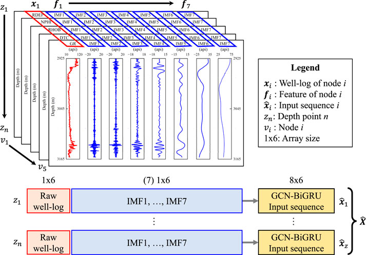
FIGURE 1. Sequence construction with the IMF features for the proposed model.

Graph construction

The S-wave velocity prediction is defined in the graph domain as follows. Given a certain number of training wells, expressed as an undirect graph $G\left(V,E\right)$, $V$ are the well-logs, $E$ are their complex dependencies, and $\mathit{X}$ are the values of the well-log curves. The goal is to learn the intrinsic relationships and predict the S-wave velocity ${\widehat{\mathit{y}}}_z$. The graph construction workflow calculates the edge weights and the graph convolution (Gconv) operator. Then, the node features are fed to the GCN-BiGRU network to output the S-wave velocity, as shown in Figure 2. Transforming well-log data into the graph domain is crucial since the Gconv operator requires reliable estimation of the graph interdependencies for an accurate prediction. Although there are no optimal methods to generate a graph from tabular data (Narayanan et al., 2017), we proposed a knowledge-based approach to aggregate information from the external domain. The edge features are calculated with the TIC to represent the complex intrinsic relationships between the physical rock properties measured by the well logs and highlight the most significant dependencies.

FIGURE 2

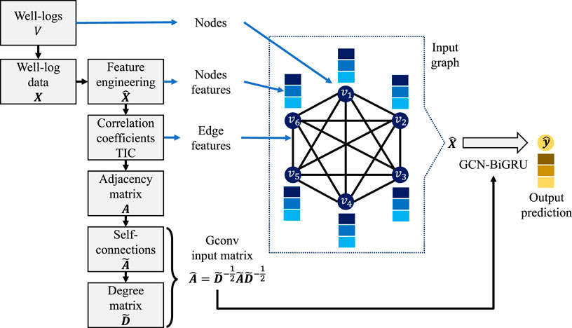
FIGURE 2. Graph construction workflow.

TIC is a variation of the maximal information coefficient (MIC) that integrates power, equitability, and performance to extract the potentially diverse relationships among well-log data (Reshef et al., 2018). MIC is a coefficient that detects non-linear dependencies by applying information theory and probability concepts and is robust to noise regardless of the relationship type (Reshef et al., 2011; Reshef et al., 2015). Mutual information (MI) is defined by the Kullback-Leibler divergence between two well logs joint and marginal distributions; the higher the variance, the higher the MI (Reshef et al., 2016). MIC is calculated by drawing a grid over a scatter plot to partition the data and embed the relationship. The well-log data distributions are discretized into bins, and the MI values are compared and divided by the theoretical maximum for a particular combination of bins. Then, MIC is defined as the highest normalized MI between two well-logs by

$\mathrm{M}\mathrm{I}\mathrm{C}\left(x,y\right)=\frac{\max \left(I\left(x,y\right)\right)}{{\mathit{log}}_2\left(\mathit{min}\left(n_x,n_y\right)\right)}(15)$

where $I\left(x,y\right)$ is the MI between the well-logs x and y, $n_x,n_y$ are the number of bins where x and y are partitioned. The MIC calculation becomes computationally expensive in large datasets. Therefore, the maximal grid size for simplification and optimization is defined by

$n_x{n}_y<B\left(n\right)=n^6(16)$

where n is the sample size. If $B\left(n\right)$ is significantly low, MIC searches only simple patterns, weakening the generality of MIC. If $B\left(n\right)$ is extremely high, MIC searches non-trivial coefficients for independent paired variables under finite samples. Therefore, MIC is redefined as

$\mathrm{M}\mathrm{I}\mathrm{C}\left(x,y\right)=\underset{n_x{n}_y\le B\left(\mathrm{n}\right)}{\max }\frac{\max \left(I\left(x,y\right)\right)}{{\mathit{log}}_2\left(\mathit{min}\left(n_x,n_y\right)\right)}(17)$

MIC measures equitability rather than the power to reject a null hypothesis of independence. Therefore, TIC is introduced to address this issue. Instead of choosing the maximal MI value, all entries are summed,

$\mathrm{T}\mathrm{I}\mathrm{C}\left(\mathrm{x},\mathrm{y}\right)={\displaystyle \sum }_{n_x{n}_y\le B\left(\mathrm{n}\right)}\frac{\max \left(I\left(\mathrm{x},\mathrm{y}\right)\right)}{{\mathit{log}}_2\left(\mathit{min}\left(n_x,n_y\right)\right)}(18)$

Finally, the prediction performance of the graph embeddings using TIC and MIC are compared with other linear and non-linear correlation coefficients. The Pearson product-moment correlation coefficient (PC) (Szabo and Dobroka, 2017) quantifies linear relationships. And the Spearman rank correlation coefficient (SC) (Pilikos and Faul, 2019) and distance correlation coefficient (DC) (Skekely et al., 2007) measure non-linear relationships.

Network architecture

The GCN-BiGRU, GCN-GRU, and GCN network structures are shown in Figure 3. In Figure 3A, the input $\widehat{\mathit{X}}$ ∈ ${\mathbb{R}}^{N\times Z}$ of the GCN-BiGRU is the feature matrix defined by well-logging data concatenated with the engineering features, where N is the number of well-log curves, and Z is the number of depth samples. The GCN-GRU predicts the spatial-temporal relationships in the forward and backward direction and transmits their final state ${\mathit{h}}_z$ to the next GCN-GRU. The final output $y_z$ is the predicted S-wave velocity at each depth point. In Figure 3B, the GCN-GRU consists of a reset gate ${\mathit{r}}_z$, an update gate ${\mathit{u}}_z$, a candidate memory ${\mathit{c}}_z$, and a GCN to extract the most relevant information between depth points and output the state ${\mathit{h}}_z$. In Figure 3C, the GCN concatenates the input node features with a hidden state, followed by the Gconv, an activation function, and a dropout layer. The Gconv captures the spatial relationships between the well-logs and hidden states within a first-order neighborhood radius. The GCN extracts spatial dependencies among nodes at each depth point, and the GCN-GRU extracts depth dependencies along depth points.

FIGURE 3

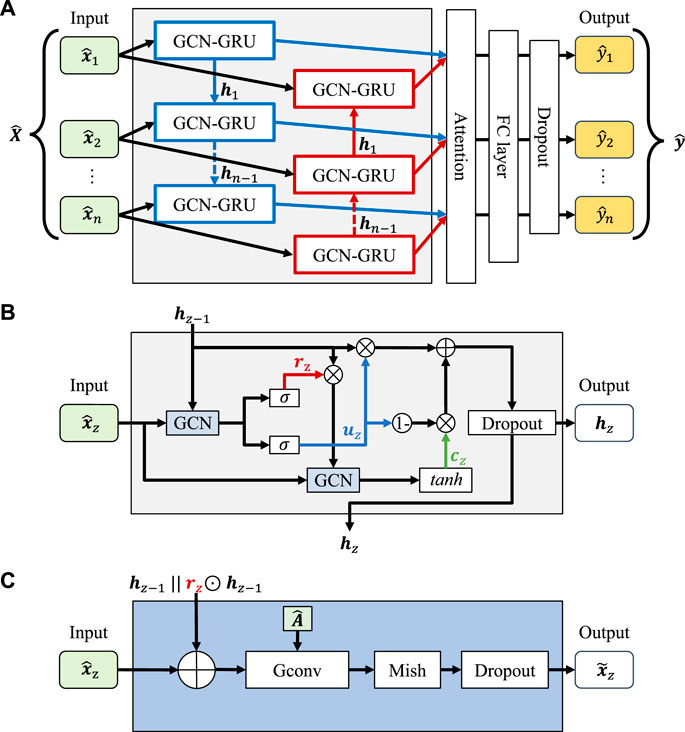
FIGURE 3. (A) GCN-BiGRU structure. (B) GCN-GRU structure. (C) GCN structure.

The Gconv uses the adjacency matrix A, degree matrix $\mathit{D}$, and feature matrix $\mathit{X}$ to construct a normalized spectral filter in the Fourier domain (Kipf and Welling, 2017). The adjacency matrix A ∈ ${\mathbb{R}}^{N\times N}$ describes the edge weights between N well-logs, defined by the calculated correlation coefficient. The diagonal matrix D∈ ${\mathbb{R}}^{N\times N}$ describes the number of edges at each node, computed from A. Then, a single-layer Gconv operator is defined by

$\text{Gconv}\left(\widehat{\mathbf{X}},\widehat{\mathbf{A}}\right)={\mathit{f}}_{\mathit{\text{drop}}}\left(\mathrm{\sigma }\left(\widehat{\mathbf{A}}\widehat{\mathbf{X}}\mathbf{W}\right)\right)(19)$

where $\widehat{\mathit{A}}$ is the normalized self-connected adjacency matrix defined as ${\widehat{\mathit{A}}=\stackrel{\sim }{\mathit{D}}}^{-\frac{1}{2}}\stackrel{\sim }{\mathit{A}}{\stackrel{\sim }{\mathit{D}}}^{-\frac{1}{2}}$, $\stackrel{\sim }{\mathit{A}}$ denotes the adjacency matrix with self-connections, defined as $\stackrel{\sim }{\mathit{A}}=\mathit{A}+\mathit{I}$, where $\mathit{I}$ is the identity matrix, $\stackrel{\sim }{\mathit{D}}$ is the degree matrix of the adjacency matrix with self-connections $\stackrel{\sim }{\mathit{A}}$, defined as $\stackrel{\sim }{\mathit{D}}={\sum }_j{\stackrel{\sim }{\mathit{A}}}_{ij}$ where i is the number of nodes, j is the number of edges, $\mathit{W}$ are the trainable weights, whose size is determined by the number of hidden units, $\sigma$(⋅) is the Mish activation function for non-linearity, and f_drop is a dropout layer with a given probability, activated during the training phase, to reduce overfitting. Mish is a novel self-regularized non-monotonic activation function that surpasses ReLU and Swish performances (Misra, 2019). Mish is defined by

$\mathrm{M}\mathrm{i}\mathrm{s}\mathrm{h}=x\tanh \left(\ln \left(1+e^x\right)\right)(20)$

The GCN-BiGRU network comprises two GCN-GRUs for a forward and backward prediction. Each GCN-GRU has a two-gated mechanism to adaptively capture patterns from different depth points (Cho et al., 2014), as shown in Figure 3B. The activation gates are the reset gate ${\mathit{r}}_z$ and the updated gate ${\mathit{u}}_z$. The GCN-GRU requires two inputs, the feature matrix ${\widehat{\mathit{x}}}_z$ at depth z and the previous hidden cell state ${\mathit{h}}_{z-1}$. First, the reset gate ${\mathit{r}}_z$ controls the amount of information to preserve from the previous depth point to transmit to the memory candidate state ${\mathit{c}}_z$. The reset gate ${\mathit{r}}_z$ combines the previous memory information ${\mathit{h}}_{z-1}$ with the current information ${\widehat{\mathit{x}}}_z$ by

${\mathit{r}}_z=\sigma \left({\mathit{W}}_r\mathrm{G}\mathrm{c}\mathrm{o}\mathrm{n}\mathrm{v}\left(\left[{\widehat{\mathit{x}}}_z,{\mathit{h}}_{z-1}\right],\mathit{A}\right)+{\mathit{b}}_r\right)(21)$

where ${\mathit{W}}_r$ and ${\mathit{b}}_r$ are the trainable parameters of the reset gate, ${\widehat{\mathit{x}}}_z$ is the current state input, ${\mathit{h}}_{z-1}$ is the hidden state from the previous depth point, [$\cdot$] represents the concatenation, $\sigma$(⋅) is the logistic sigmoid function that forces the output range between [0,1], ${\mathit{r}}_z$ output is a scalar, ${\mathit{r}}_z\in$ [0,1], when ${\mathit{r}}_z=1$ the memory is preserved, when ${\mathit{r}}_z=0,$ the memory is discarded. Second, the update gate ${\mathit{u}}_z$ determines the amount of information to preserve from the previous depth point and the amount of current information to include from the current depth point, similar to the reset gate,

${\mathit{u}}_z=\sigma \left({\mathit{W}}_u\mathrm{G}\mathrm{c}\mathrm{o}\mathrm{n}\mathrm{v}\left(\left[{\widehat{\mathit{x}}}_z,{\mathit{h}}_{z-1}\right],\mathit{A}\right){+\mathit{b}}_u\right)(22)$

where ${\mathit{W}}_u$, and ${\mathit{b}}_u$ are the trainable parameters of the update gate. Third, the memory candidate ${\mathit{c}}_z$ is the present moment state at the depth point z and is defined by

${\mathit{c}}_z=\tanh \left({\mathit{W}}_c\mathrm{G}\mathrm{c}\mathrm{o}\mathrm{n}\mathrm{v}\left(\left[{\widehat{\mathit{x}}}_z,\left({{\mathit{r}}_z\odot \mathit{h}}_{z-1}\right)\right],\mathit{A}\right)+{\mathit{b}}_c\right)(23)$

where ${\mathit{W}}_c$, ${\mathit{b}}_c$ are the trainable parameters of the candidate memory, $\odot$ is the Hadamard product (i.e., element-wise multiplication), and $\tanh$ is the hyperbolic tangent function. Finally, the output state ${\mathit{h}}_z$ at depth z is defined by

${\mathit{h}}_z=\left(1-{\mathit{u}}_z\right)\odot {\mathit{c}}_z+{\mathit{u}}_z\odot {\mathit{h}}_{z-1}(24)$

The update gate selectively stores or forgets memory information. The update gate acts as a forget gate when ${\mathit{u}}_z\odot {\mathit{h}}_{z-1}$ ignores unimportant information from the previous depth point. The update gate acts as a memory gate when $\left(1-{\mathit{u}}_z\right)\odot {\mathit{c}}_z$ preserves relevant information in memory for the next depth point. Additionally, a dropout layer is added at the end of each GCN-GRU to increase the network generalization ability and reduce overfitting. Next, the output state ${\mathit{h}}_z$ is fed into a hierarchical attention mechanism to highlight the essential features and attenuate the less significative information contributing to the S-wave velocity prediction (Bahdanau et al., 2014; Yang et al., 2016). The output state ${\mathit{h}}_z$ is fed into a fully connected (FC) layer, followed by an activation function to obtain a hidden representation ${\mathit{u}}_z$ defined by

${\mathit{u}}_z=\tanh \left({\mathit{W}}_a{\mathit{h}}_z+{\mathit{b}}_a\right)(25)$

where ${\mathit{W}}_a$ and ${\mathit{b}}_a$ are the trainable parameters of the FC layer. Next, the feature importance is measured between the hidden representation ${\mathit{u}}_z$ and a trainable context vector ${\mathit{u}}_w$ that is a high-level representation of a static query of the features (Sukhbaatar et al., 2015; Kumar et al., 2016). Then, importance weights are normalized through a softmax function ${\mathit{\alpha }}_z$ by

${\mathit{\alpha }}_z=\frac{\exp \left({\mathit{u}}_z{\mathit{u}}_w\right)}{{\displaystyle \sum }_z\exp \left({\mathit{u}}_z{\mathit{u}}_w\right)}(26)$

Then, the weighted sum of the hidden states is the new high-level presentation of the output state ${\widehat{\mathit{h}}}_z$ and is defined by

${\widehat{\mathit{h}}}_z={\displaystyle \sum }_z{\mathit{\alpha }}_z{\mathit{h}}_z(27)$

and the new output state ${\widehat{\mathit{h}}}_z$ is fed to a fully connected (FC) layer with a Mish activation function and a dropout layer to predict the S-wave velocity by

${\widehat{y}}_z={\mathit{f}}_{\mathit{\text{drop}}}\left(\sigma \left({\mathit{W}}_f{\widehat{\mathit{h}}}_z+{\mathit{b}}_f\right)\right)(28)$

where ${\mathit{W}}_f$ and ${\mathit{b}}_f$ are the trainable parameters of the final FC layer. Lastly, the training dataset is rearranged into sequences in the supervised training process and matched with the labels. The Huber loss function is implemented to minimize the difference between the predicted S-wave velocity ${\widehat{y}}_z$ and the actual S-wave velocity $y_z$ at depth z. The Huber loss is less sensitive to outliers and noise by combining L1 and L2 norms (Yu et al., 2016) and is defined by

$\mathcal{L}=\left\{\begin{array}{c}{\frac{1}{2}\left(y_z{-\widehat{y}}_z\right)}^2,\left|y_z{-\widehat{y}}_z\right|\le \delta \\ \delta \left(\left|y_z{-\widehat{y}}_z\right|-\frac{1}{2}\delta \right),\left|y_z{-\widehat{y}}_z\right|>\delta \end{array}\right.(29)$

where $\delta =0.1$ is the threshold parameter for the L1/L2 norm. The adaptive movement estimation algorithm (Adam) is used for network optimization with a learning rate of 0.001 (Kingma and Ba, 2015). The grid search strategy is applied to optimize the network parameters selection and a 10-fold cross-validation method to evaluate the accuracy and generalization ability of the model while reducing randomness impact (Hampson et al., 2001). Finally, the metrics to evaluate the difference between the actual S-wave velocity and the predicted S-wave velocity are RMSE, MAE, MAPE, and R². RMSE measures the average weighted performance of the model. MAE estimates the average error of the model for the prediction. MAPE measures the percentage of the average difference between the actual and the predicted value. The coefficient of determination measures the performance of the model over a regressor that outputs the mean value of the label that is used in training. The error metrics are defined as follows,

$\mathrm{R}\mathrm{M}\mathrm{S}\mathrm{E}=\sqrt{\frac{1}{N}{\sum }_{z=1}^N{\left(y_z-{\widehat{y}}_z\right)}^2}(30)$

$\mathrm{M}\mathrm{A}\mathrm{E}=\frac{1}{N}{\sum }_{z=1}^N\left|y_z-{\widehat{y}}_z\right|(31)$

$\mathrm{M}\mathrm{A}\mathrm{P}\mathrm{E}=\frac{1}{N}{\sum }_{z=1}^N\frac{\left|y_z-{\widehat{y}}_z\right|}{\left|y_z\right|}\times 100(32)$

${\mathrm{R}}^2=1-\frac{{\sum }_{z=1}^N{\left(y_z-{\widehat{y}}_z\right)}^2}{{\sum }_{z=1}^N{\left(y_z-\overline{y}\right)}^2}(33)$

where $\overline{y}$ is the mean of the actual S-wave velocity, and N is the number of samples.

Field data example

The study comprises a selection of 30 wells from the North Sea area (Bormann et al., 2020). The training dataset consists of 21 wells, the validation dataset includes 5 wells, and the testing dataset consists of 4 blind wells. Each well has 6 well-log curves: Gamma-ray (GR), compressional wave transit-time (DTC), shear wave transit-time (DTS), bulk density (RHOB), neutron porosity (NPHI), and deep resistivity (RDEP). The original sampling interval is 0.152 m, and the range of the training dataset is constrained for stability purposes, as shown in Table 1. The GCN-BiGRU employs a prediction window of 1 sample, a sequence length of 8 samples, and 8 hidden units for the dimension of the hidden state. The training time is 20 min for 50 epochs and a batch size of 128 samples in an Nvidia GeForce GTX 960M.

TABLE 1

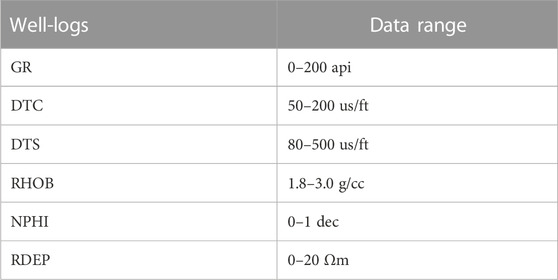
TABLE 1. Well-log data range for the training dataset.

Additionally, the robustness of the proposed method is evaluated by measuring the impact of the proportion of the training dataset and the sensitivity to Gaussian noise. First, the training dataset is divided into ten groups based on the number of wells (i.e., 4, 7, 9, 10, 12, 15, 16, 17, 20, and 21), corresponding to a ratio of 0.1, 0.2, 0.3, 0.4, 0.5, 0.6, 0.7, 0.8, 0.9, and 1 of the training dataset, respectively. Second, the noise resistance is analyzed by adding Gaussian noise with mean zero and standard deviation of the training dataset (i.e., σ_GR = 40.96 api, σ_DTC = 20.09 us/ft, σ_DTS = 79.20 us/ft, σ_RHOB = 0.17 g/cc, σ_NPHI = 0.10 dec, σ_RDEP = 21.07 Ωm) to each sample. Then, the performance is evaluated by examining ten fraction levels of the defined noise (i.e., 0.1, 0.2, 0.3, 0.4, 0.5, 0.6, 0.7, 0.8, 0.9, and 1). Finally, the RMSE on the validation and testing datasets is calculated for both analyses.

The effects of the GNN, LOF, and IF methods are shown in Figure 4. GNN uses 13 samples as neighbors, LOF 50 nodes as neighbors, and IF 100 estimators. Additionally, a contamination value of 0.1 is employed for the three methods. The GNN handles the spikes located on the RHOB log below the 2,200 m better than the alternative outlier removal methods and other abrupt values on the rest of the well-logs below the 2,400 m while preserving the essential well-log information, as shown in Figure 4. In the prediction performance, the GNN surpasses LOF and IF methods, with lower RMSE error for the predicted DTS log, as shown in Figure 5. The RMSE for the training, validation and testing dataset with the GNN are 21.0482 us/ft, 22.7562 us/ft, and 23.5854 us/ft, respectively. Compared with the LOF and IF methods, the main drawback of GNN is the higher computation time.

FIGURE 4

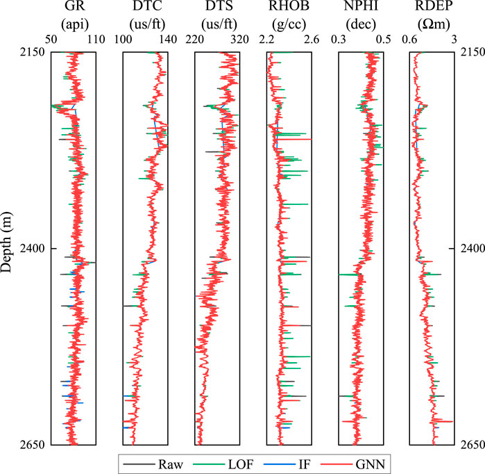
FIGURE 4. Comparison of the three methods for outlier removal at well W3.

FIGURE 5

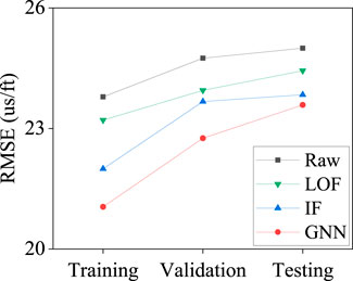
FIGURE 5. RMSE of predicted DTS for the three outlier removal methods.

The cross-plot between the DTS and the well-log curves is shown in Figure 6. The color represents the distribution density of the samples. The higher the density, the higher the color intensity. And the line represents the minimum squares regression line. The RHOB and NPHI show a good linear trend, the DTC behaves linearly for low values, and the relationship changes for higher values. The DEPT and RDEP trend is logarithmic, while the GR is unclear due to the bimodal distribution between sand and shales. The cross-plot shows that a linear correlation coefficient is insufficient to capture the intrinsic relationships of the rock properties and to build a meaningful graph structure. Therefore, a non-linear correlation coefficient is more suitable for this task.

FIGURE 6

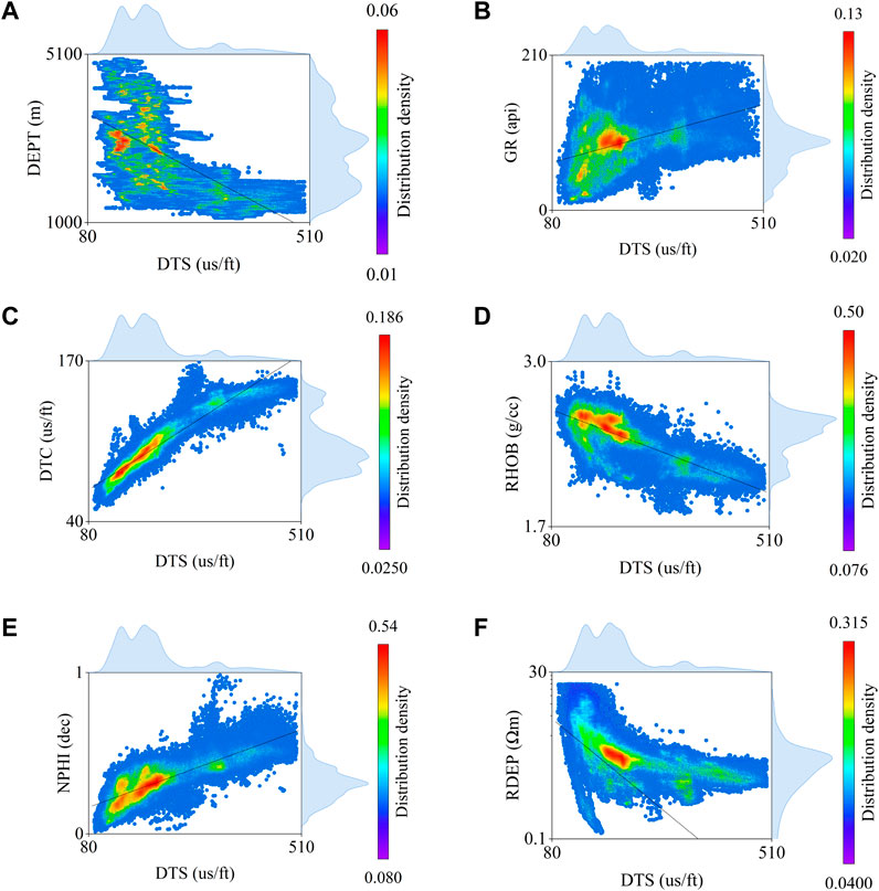
FIGURE 6. Cross plots between DTS and the well-logs. (A) DEPT. (B) GR. (C) DTC. (D) RHOB. (E) NPHI. (F). RDEP.

The relationship strength between the DTS log and the other well logs curves with the six correlation coefficients is shown in Figure 7. The hexagons range from 0 to 1, with an increment of 0.2. The closer to the center, the lower the correlation; the closer to the edges, the higher the correlation. On average, the DTC, NPHI, and RHOB logs show a high correlation, consistent with the definition of S-wave velocity. The DTC correlation is higher because it shares the shear modulus and density parameters. The density is a very sensitive parameter for rock velocity, and the porosity directly impacts the rigidity of the rock and reduces its value. The DEPT shows a moderate correlation due to the dependency on changes in pressure and temperature that affect the rock properties. RDEP has an average correlation linked to the lithology characteristics of the layer. In contrast, the low correlation in GR is probably due to averaging effect between sand and shale lithologies. These results constitute the building block to constructing a graph with meaningful physical rock relationships, proven by external knowledge.

FIGURE 7

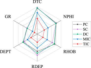
FIGURE 7. The correlation coefficients between DTS and the others well-log curves.

The evaluation of the prediction results for the six correlation coefficients is shown in Figure 8. TIC accuracy is higher than other approaches, with an RMSE value of 22.1603 us/ft, 23.3468 us/ft, and 24.2019 us/ft for the training, validation, and testing datasets, respectively. TIC is more reliable for embedding the non-linear physical correlation between the rock properties and the well-logs into the graph edges. However, MI approaches have a high computational cost for extensive datasets than other correlation coefficients. The TIC matrix used as the adjacency matrix to represent the edge features in the proposed method is shown in Figure 9. The DTC and DTS are the only pair that achieves a high correlation, with a value of 0.57, which is consistent with the theoretical and empirical results for S-wave velocity prediction.

FIGURE 8

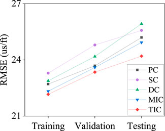
FIGURE 8. RMSE of predicted DTS of the six correlation coefficients.

FIGURE 9

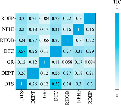
FIGURE 9. TIC for the training dataset.

The evaluation of the three feature engineering methods for the DTS log prediction is shown in Figure 10. The gradient method adds the first derivative as a component. The frequency band method uses three components. The low-frequency band (i.e., 20 Hz) isolates the significant geological trend changes. The middle-frequency band (i.e., 40 Hz) is related to third-order sequence events, while the high-frequency band (i.e., 200 Hz) focuses on the local changes inside the geological formations. After experimentation with the training dataset, the CEEMDAN method decomposes the data into 7 IMFs. This number preserves the uniformity size in all the IMFs for the sequence aggregation step and reduces overfitting by avoiding high-order IMFs without a reliable meaning. Results show that the feature engineering method can improve the prediction accuracy of the GCN-BiGRU network. The gradient shows the lowest performance because the contribution of its high frequency is less significant for the prediction. Although the computational time for the IMFs is longer than other methods, the RMSE is lower, with 20.3805 us/ft, 23.1001 us/ft, and 23.3531 us/ft, for the training, validation, and testing datasets, respectively.

FIGURE 10

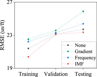
FIGURE 10. RMSE of predicted DTS for the three feature engineering methods.

The results for the DTS log prediction during the network optimization are shown in Figure 11. The RMSE of the GCN-BiGRU network is 19.6581 us/ft, 23.5363 us/ft, and 24.3045 us/ft for the training, validation, and testing datasets, respectively, improving the performance compared with the original GCN-GRU network (Zhao et al., 2020), as shown in Figure 11A. The Mish activation function shows superior regularization and overfitting reduction abilities than other state-of-the-art activation functions, such as Leaky ReLU, GELU, SELU, and Swish. The RMSE with the Mish activation function is 21.3972 us/ft, 23.1146 us/ft, and 23.6318 us/ft for the testing, validation, and testing datasets, respectively, as shown in Figure 11B.

FIGURE 11

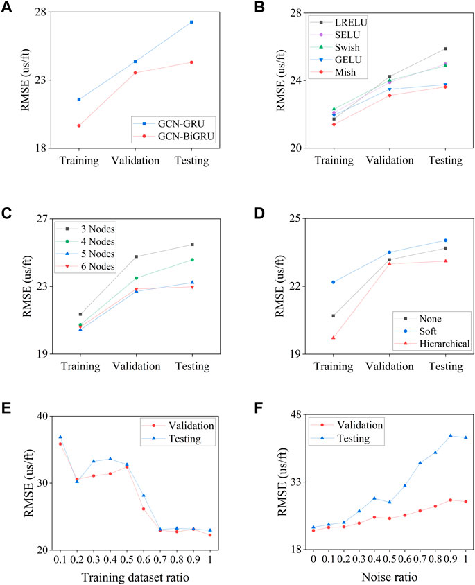
FIGURE 11. Proposed method optimization. (A). Network structure. (B) Activation Function, (C) Nodes number, (D) Attention mechanism, (E) Training ratio test, (F) Noise sensitivity test.

The prediction performance by the number of well-logs is shown in Figure 11C. The node configurations are tested based on their coefficient ranking. Thus, the GR log is excluded. The node configurations are defined as follows: The 3 nodes include the DTC, NPHI, and RHOB logs. The 4 nodes include the DTC, NPHI, RHOB, and RDEP logs. The 5 nodes include the DTC, NPHI, RHOB, RDEP, and DEPT logs. The 6 nodes include all logs. Although the RMSE error decreases with 5 nodes for the training and validation datasets, the overall performance of the GCN-BiGRU decreases for the testing dataset. The RMSE for 6 nodes is 20.6117 us/ft, 22.8539 us/ft, and 22.9764 us/ft for the training, validation, and testing datasets, respectively. The 6 nodes are used since the GCN extracts meaningful embeddings based on the number of adjacent nodes for aggregation. When the number of nodes is reduced, the GCN embeddings are shallower, and the ability to map complex physical relationships among the input data is also reduced. Then, the prediction is compared with two attention mechanisms. The hierarchical attention shows a lower RMSE than soft attention, with a value of 19.7153 us/ft, 22.9858 us/ft, and 23.1156 us/ft, for the training, validation, and testing datasets, respectively, as shown in Figure 11D. However, the attention mechanism occasionally creates spike artifacts.

The impact of the proportion of the training dataset ratio is shown in Figure 11E. The RMSE is higher for a ratio of 0.1, with a value of 35.8539 us/ft for the validation dataset and 36.8711 us/ft for the testing dataset. The RMSE reduces between a ratio of 0.2–0.5, reaching a value of 32.4315 us/ft for the validation dataset and 32.7639 us/ft for the testing dataset at a ratio of 0.5. The RMSE shows a stability plateau between a ratio of 0.7–1, achieving a value of 22.2465 us/ft for the validation dataset and 22.9672 us/ft for the testing dataset at a ratio of 1.

The prediction performance in the presence of Gaussian noise is shown in Figure 11F. The RMSE is high when the added noise is equal to the standard deviation of the training dataset (i.e., a noise fraction of 1) with a value of 28.6670 us/ft for the validation dataset and 42.8739 us/ft for the testing dataset. The RMSE gradually decreases until a noise fraction of 0.5 with a value of 24.9382 us/ft for the validation dataset and 28.5342 us/ft for the testing dataset. The RMSE is stable when the noise fraction is lower than 0.2, with a value of 22.9373 us/ft for the validation dataset and 23.5910 us/ft for a noise fraction of 0.1.

Finally, the DTS log prediction results for all the models are shown in Figure 12. The GCN-BiGRU shows lower error in the training, validation, and testing dataset with an RMSE of 19.3260 us/ft, 22.4905 us/ft, and 22.7120 us/ft, respectively. The evaluation for the testing dataset is shown in Table 2. The GCN-BiGRU shows an MAE of 17.2842 us/ft, MAPE of 6.7880%, and R² of 0.9470. The GCN-BiGRU performs better than other ML baseline models and empirical equations without adding mineral components, fluid properties, pore aspect ratio, or thermal maturity information. Some discrepancies in the predicted DTS log and the actual DTS log value are due to the presence of fluids, unbalanced lithologies samples, or the inherent covariance shift problem.

FIGURE 12

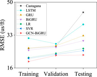
FIGURE 12. RMSE of the predicted DTS for all the compared methods.

TABLE 2

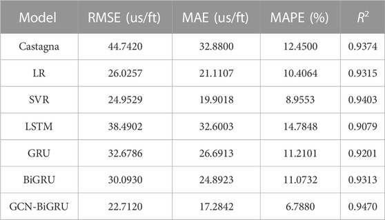
TABLE 2. DTS prediction results for the testing dataset.

The results for the testing well B9 are shown in Figure 13. The predicted DTS log is consistent with the actual DTS log, as shown in Figure 13A. The model performs satisfactorily when constant or missing values are present, such as the depths 2,900 m, 3,100 m, and 3,400 m. The distribution of the predicted DTS and the true DTS are consistent, as shown in Figure 13B. The range of the predicted DTS for higher values is reduced due to the constraints established during the training phase. The R² coefficient between the true and predicted DTS is 0.9593, as shown in Figure 163. The high coefficient indicates that the proposed model can explain a significant variation in the actual DTS log. Moreover, the homoscedasticity analysis shows that the variance of the residuals is homogeneous, thus increasing the robustness and feasibility of the method, as shown in Figure 13D.

FIGURE 13

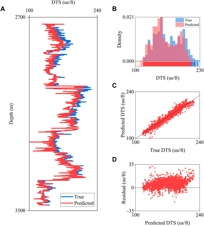
FIGURE 13. DTS prediction results on testing well B9. (A) DTS log curve, (B) True and predicted DTS distribution, (C) R² analysis, (D) Homoscedasticity analysis.

Discussion

The proposed GCN-BiGRU method predicts the S-wave velocity by extracting the spatial and depth relationships among well-log data. The model combines GCN into GRU to create a GCN-GRU network, which is implemented to predict the S-wave velocity in two directions, forming the GCN-BiGRU network. The performance of the method is evaluated with a training dataset ratio test and a noise sensitivity test. The GCN-BiGRU has a lower error than Castagna’s equation, LR, SVR, LSTM, GRU, and BiGRU baseline methods using the well-logs from the North Sea area. The approach is feasible and could be further extended for reservoir properties prediction using inverted seismic data as input and output maps and volumes of rock properties.

The GCN embeds the topological information, the intrinsic relationships, and the measured physical properties of the geological formations by an external-knowledge approach. The Gconv aggregates nearby information from the nodes, resembling a spectral Fourier filter. The number of nodes in the graph impacts the quality of the embeddings. Fewer nodes create shallow embeddings that reduce the representation ability.

Although 1-layer GCN is adopted due to the current graph topology, the GCN can extract deeper patterns from the well-log data with multiple GCN layers (Magner et al., 2022). Further research could reframe the graph creation process and add more hierarchy nodes (i.e., nodes connected below the first-level nodes) for a meaningful aggregation during the graph embeddings.

The GCN-GRU extracts patterns over previous data windows to map the changes in rock properties with depth. The number of hidden units inside the GCN-GRU impacts the ability to memorize the most important information for the S-wave velocity prediction. Moreover, the dimension of the hidden states balances the generalization and overfitting of the GCN-GRU.

GNNs are a versatile approach to solving problems by the intrinsic message-passing characteristic. As an unsupervised outlier removal method, GNN shows promising results in handling anomalous values based on the sample distance between neighbor samples. GNN adapts to particular datasets by fine-tuning the number of nearest neighbor samples, which is essential for the detection performance. GNN for local outlier removal increases the accuracy of the model at the expense of a higher computational cost than IF and LOF.

The feature engineering process improves the prediction ability of the GCN-BiGRU. The prediction error is reduced with the IMFs. However, the network complexity and the training time increase with a higher number of features. The frequency bands are an alternative trade-off between accuracy and efficiency.

The construction of the graph is an essential step for the success of graph embedding. The proposed approach constructs the adjacency matrix from the correlation coefficients among well-log data. This supervised external-knowledge approach links the relationships between the measured rock properties and the wave propagation parameters into the network. Linear coefficients have limitations for capturing intrinsic rock dependencies and are more sensitive to their variation with depth. Non-linear coefficients extract suitable representations of the complex relationships between rocks and measured physical properties and are more robust to well-log data variance, preserving the intrinsic dependencies that govern depth.

Depth changes are affected by temperature, pressure, fluid, and lithology, among other factors. Difficulties arise with a fixed adjacency matrix in complex geological scenarios by approximating the global properties variation with depth. Specifically, the GCN has limitations for predicting local minima and maxima due to the smooth moving average filter in the Fourier domain. Therefore, further research towards a dynamic graph representation to recreate more realistic models and map depth-dependent representations is encouraged.

The GCN-BiGRU uses point-wise activation functions as a non-linear operator. Nevertheless, further research is required to adapt non-linearities directly into the graph domain and increase the generalization of the model. The contribution of conventional attention mechanisms for the S-wave velocity prediction should be further explored. Graph attention networks or graph transformers have the potential to improve the ability of the network in abrupt lithology changes.

Conclusion

This study introduces a novel method for predicting S-wave velocity with a GCN-BiGRU network. GCN captures the spatial dependencies from the well-log data, while bidirectional GCN-GRU maps the changes in the rock properties with depth in both upward and backward directions. The well-log data are transformed into the graph domain by integrating external knowledge into the model. The well-logs are the graph nodes, well-logging data are the node features, and their intrinsic non-linear relationships are the edges features defined by TIC. Moreover, an unsupervised GNN is implemented for outlier removal to increase the network performance. And IMFs are aggregated to the node features, improving the prediction accuracy. The proposed method performs better than LR, SVR, LSTM, GRU, BiGRU methods, and Castagna’s empirical equation. Finally, this method shows promising applications for predicting reservoir properties using inverted seismic data.

Data availability statement

The original contributions presented in the study are included in the article/Supplementary Material, further inquiries can be directed to the corresponding author. The North Sea dataset can be downloaded through the dGB Earth Sciences Open Seismic Repository https://terranubis.com/datainfo/FORCE-ML-Competition-2020-Synthetic-Models-and-Wells.

Author contributions

DC and YL contributed to the idea and methodology. DC was responsible for the field data training and testing and the writing of the manuscript, and YL checked and polished the manuscript. All authors have read the manuscript and agreed to publish it.

Funding

National Natural Science Foundation of China (NSFC) under contract no. 42274147.

Acknowledgments

We want to thank the Editor, Zhenming Peng, and the two external peer reviewers for their insightful comments and suggestions, which helped improve the quality of our manuscript. We also thank Gui Cheng for his helpful discussion and valuable recommendations. We are particularly grateful to China’s National Natural Science Foundation for its founding and support.

Conflict of interest

The authors declare that the research was conducted in the absence of any commercial or financial relationships that could be construed as a potential conflict of interest.

Publisher’s note

All claims expressed in this article are solely those of the authors and do not necessarily represent those of their affiliated organizations, or those of the publisher, the editors and the reviewers. Any product that may be evaluated in this article, or claim that may be made by its manufacturer, is not guaranteed or endorsed by the publisher.

References

Ali, M., Jiang, R., Ma, H., Pan, H., Abbas, K., Ashraf, U., et al. (2021). Machine learning – a novel approach of well logs similarity based on synchronization measures to predict shear sonic logs. J. Pet. Sci. Eng. 203, 108602. doi:10.1016/j.petrol.2021.108602

CrossRef Full Text | Google Scholar

Amarbayasgalan, T., Jargalsaikhan, B., and Ryu, K. H. (2018). Unsupervised novelty detection using deep autoencoders with density based clustering. Appl. Sci. 8 (9), 1468. doi:10.3390/app8091468

CrossRef Full Text | Google Scholar

Anemangely, M., Ramezanzadeh, A., Amiri, H., and Hoseinpour, S. (2019). Machine learning technique for the prediction of shear wave velocity using petrophysical logs. J. Pet. Sci. Eng. 174, 306–327. doi:10.1016/j.petrol.2018.11.032

CrossRef Full Text | Google Scholar

Bahdanau, D., Cho, K., and Bengio, Y. (2014). Neural machine translation by jointly learning to align and translate. ArXiv abs/1409.0473.

Google Scholar

Bormann, P., Aursand, P., Dilib, F., Dischington, P., and Manral, S. (2020). FORCE Mach. Learn contest. Avaliable At: https://github.com/bolgebrygg/Force-2020-Machine-Learning-competition.

Google Scholar

Breunig, M. M., Kriegel, H. P., Ng, R. T., and Sander, J. (2000). Lof: Identifying density-based local outliers. ACM SIGMOD Rec. 29 (2), 93–104. doi:10.1145/342009.335388

CrossRef Full Text | Google Scholar

Castagna, J. P., Batzle, M. L., and Eastwood, R. L. (1985). Relationships between compressional-wave and shear-wave velocities in clastic silicate rocks. Geophysics 50 (4), 571–581. doi:10.1190/1.1441933

CrossRef Full Text | Google Scholar

Chen, W., Yang, L., Zha, B., Zhang, M., and Chen, Y. (2020). Deep learning reservoir porosity prediction based on multilayer long short-term memory network. Geophysics 85 (4), WA213–WA225. doi:10.1190/geo2019-0261.1

CrossRef Full Text | Google Scholar

Cho, K., Merrienboer, B., Bahdanau, D., and Bengio, Y. (2014). “On the properties of neural machine translation: Encoder-decoder approaches,” in Proc. Syntax semant. Struct. Stat. Transl (Doha, Qatar: Association for Computational Linguistics), 103–111. doi:10.3115/v1/W14-4012

CrossRef Full Text | Google Scholar

Colominas, M. A., Schlotthauer, G., and Torres, M. E. (2014). Improved complete ensemble EMD: A suitable tool for biomedical signal processing. Biomed. Signal Process. Control. 14 (1), 19–29. doi:10.1016/j.bspc.2014.06.009

CrossRef Full Text | Google Scholar

Defferrard, M., Bresson, X., and Vandergheynst, P. (2016). “Convolutional neural networks on graphs with fast localized spectral filtering,” in Proc. Int. Conf. Neural inf. Process. Syst, Barcelona, Spain, December 5–10, 2016 (Neural Information Processing Systems (NIPS)), 3844–3852. doi:10.5555/3157382.3157527

CrossRef Full Text | Google Scholar

Di Massa, V., Monfardini, G., Sarti, L., Scarselli, F., Maggini, M., and Gori, M. (2006). “A comparison between recursive neural networks and graph neural networks,” in Proc. Int. Jt. Conf. Neural Netw, Vancouver, BC, Canada, 16-21 July 2006 (IEEE), 778–785. doi:10.1109/IJCNN.2006.246763

CrossRef Full Text | Google Scholar

Gao, H., Jia, H., and Yang, L. (2022). An improved CEEMDAN-FE-TCN model for highway traffic flow prediction. J. Adv. Transp. 2022, 1–20. doi:10.1155/2022/2265000

CrossRef Full Text | Google Scholar

Goodge, A., Hooi, B., Ng, S. K., and Ng, W. S. (2022). Lunar: Unifying local outlier detection methods via graph neural networks. Proc. AAAI Conf. Artif. Intell. 36 (6), 6737–6745. doi:10.1609/aaai.v36i6.20629

CrossRef Full Text | Google Scholar

Gori, M., Monfardini, G., and Scarselli, F. (2005). A new model for learning in graph domains. Proc. Int. Jt. Conf. Neural. Netw. 2, 729–734. doi:10.1109/IJCNN.2005.1555942

CrossRef Full Text | Google Scholar

Greenberg, M. L., and Castagna, J. P. (1992). Shear-wave velocity estimation in porous rocks: Theoretical formulation, preliminary verification and applications. Geophys. Prospect 40 (2), 195–209. doi:10.1111/j.1365-2478.1992.tb00371.x

CrossRef Full Text | Google Scholar

Hamilton, W. L., Ying, R., and Leskovec, J. (2017). “Inductive representation learning on large graphs,” in Proc. Int. Conf. Neural syst, Long Beach, California, United States, December 4–9, 2017 (Neural Information Processing Systems (NIPS)), 1025–1035. doi:10.5555/3294771.3294869

CrossRef Full Text | Google Scholar

Hampson, D., Schuelke, J. S., and Quirein, J. (2001). Use of multiattribute transforms to predict log properties from seismic data. Geophysics 66 (1), 220–236. doi:10.1190/1.1444899

CrossRef Full Text | Google Scholar

Hopfield, J. J. (1982). Neural networks and physical systems with emergent collective computational abilities. Proc. Natl. Acad. Sci. USA. 79 (8), 2554–2558. doi:10.1073/PNAS.79.8.2554

PubMed Abstract | CrossRef Full Text | Google Scholar

Huang, N. E., Shen, Z., Long, S. R., Wu, M. L. C., Shih, H. H., Zheng, Q., et al. (1998). The empirical mode decomposition and the Hilbert spectrum for non-linear and non-stationary time series analysis. Proc. R. Soc. Lond. 454, 903–995. doi:10.1098/rspa.1998.0193

CrossRef Full Text | Google Scholar

Jiang, C., Zhang, D., and Chen, S. (2021). Lithology identification from well-log curves via neural networks with additional geologic constraint. Geophysics 86 (5), IM85–IM100. doi:10.1190/geo2020-0676.1

CrossRef Full Text | Google Scholar

Jiang, S., Liu, X., Xing, J., and Liang, L. (2018). “Study of S-wave velocity prediction model in shale formations,” in SEG global meeting abstr (Beijing, China: SEG Global Meeting), 1343–1345. doi:10.1190/IGC2018-329

CrossRef Full Text | Google Scholar

Kingma, D. P., and Ba, J. (2015). Adam: A method for stochastic optimization. ArXiv abs/1412.6980.

Google Scholar

Kipf, T., and Welling, M. (2017). Semi-supervised classification with graph convolutional networks. ArXiv abs/1609.02907.

Google Scholar

Kumar, A., Irsoy, O., Su, J., Bradbury, J., English, R., Pierce, B., et al. (2016). Ask me anything: Dynamic memory networks for natural language processing. Proc. Int. Conf. Neural Inf. Process. Syst. 48, 1378–1387. doi:10.5555/3045390.3045536

CrossRef Full Text | Google Scholar

Liu, F. T., Ting, K. M., and Zhou, Z. H. (2008). “Isolation forest,” in IEEE Int. Conf. Data Min, Pisa, Italy, 15-19 December 2008 (IEEE), 413–422. doi:10.1109/ICDM.2008.17

CrossRef Full Text | Google Scholar

Magner, A., Baranwal, M., and Hero, A. O. (2022). Fundamental limits of deep graph convolutional networks for graph classification. IEEE Trans. Inf. Theory 68 (5), 3218–3233. doi:10.1109/TIT.2022.3145847

CrossRef Full Text | Google Scholar

Misra, D. (2019). Mish: A self regularized non-monotonic activation function. ArXiv abs/1908.08681.

Google Scholar

Narayanan, A., Chandramohan, M., Venkatesan, R., Chen, L., Liu, Y., and Jaiswal, S. (2017). Graph2vec: Learning distributed representations of graphs. ArXiv abs/1707.05005.

Google Scholar

Ni, W., Qi, L., and Tao, F. (2017). “Prediction of shear wave velocity in shale reservoir based on logging data and machine learning,” in Proc. Int. Conf. Softw. Eng. Knowl. Eng, London, UK, 21-23 October 2017 (IEEE), 231–234. doi:10.1109/ICKEA.2017.8169935

CrossRef Full Text | Google Scholar

Omovie, S. J., and Castagna, J. P. (2021). Estimation of shear-wave velocities in unconventional shale reservoirs. Geophys. Prospect. 69 (6), 1316–1335. doi:10.1111/1365-2478.13096

CrossRef Full Text | Google Scholar

Pilikos, G., and Faul, A. C. (2019). Bayesian modeling for uncertainty quantification in seismic compressive sensing. Geophysics 84 (2), P15–P25. doi:10.1190/geo2018-0145.1

CrossRef Full Text | Google Scholar

Refunjol, X. E., Wallet, B. C., and Castagna, J. P. (2022). Fluid discrimination using detrended seismic impedance. Interpretation 10 (1), SA15–SA24. doi:10.1190/INT-2020-0219.1

CrossRef Full Text | Google Scholar

Reshef, D. N., Reshef, Y. A., Finucane, H. K., Grossman, S. R., Mcvean, G., Turnbaugh, P. J., et al. (2011). Detecting novel associations in large data sets. Science 334 (6062), 1518–1524. doi:10.1126/science.1205438

PubMed Abstract | CrossRef Full Text | Google Scholar

Reshef, D. N., Reshef, Y. A., Sabeti, P. C., and Mitzenmacher, M. (2018). An empirical study of the maximal and total information coefficients and leading measures of dependence. Ann. Appl. Stat. 12 (1), 123–155. doi:10.1214/17-AOAS1093

CrossRef Full Text | Google Scholar

Reshef, Y. A., Reshef, D. N., Sabeti, P. C., and Mitzenmacher, M. (2015). Equitability, interval estimation, and statistical power. ArXiv abs/1505.022122015.

Google Scholar

Reshef, Y. A., Reshef, D. N., Sabeti, P. C., and Mitzenmacher, M. (2016). Measuring dependence powerfully and equitably. J. Mach. Learn. Res. 17 (1), 7406–7468. doi:10.5555/2946645.3053493

CrossRef Full Text | Google Scholar

Scarselli, F., Gori, M., Tsoi, A. C., Hagenbuchner, M., and Monfardini, G. (2009). The graph neural network model. IEEE Trans. Neural Netw. 20 (1), 61–80. doi:10.1109/TNN.2008.2005605

PubMed Abstract | CrossRef Full Text | Google Scholar

Skekely, G. J., Rizzo, M. L., and Bakirov, N. K. (2007). Measuring and testing dependence by correlation of distances. Ann. Stat. 35 (6), 2769–2794. doi:10.1214/009053607000000505

CrossRef Full Text | Google Scholar

Sukhbaatar, S., Szlam, A., Weston, J., and Fergus, R. (2015). End-to-end memory networks. Proc. Int. Conf. Neural Inf. Process. Syst. 2, 2440–2448. doi:10.5555/2969442.2969512

CrossRef Full Text | Google Scholar

Sun, Y., and Liu, Y. (2020). Prediction of S-wave velocity based on GRU neural network. Oil Geophys. Prospect. 55 (3), 484–492. doi:10.13810/j.cnki.issn.1000-7210.2020.03.001-en

CrossRef Full Text | Google Scholar

Szabó, N. P., and Dobroka, M. (2017). Robust estimation of reservoir shaliness by iteratively reweighted factor analysis. Geophysics 82 (2), D69–D83. doi:10.1190/geo2016-0393.1

CrossRef Full Text | Google Scholar

Vernik, L., Castagna, J., and Omovie, S. J. (2018). S-wave velocity prediction in unconventional shale reservoirs. Geophysics 83 (1), MR35–MR45. doi:10.1190/geo2017-0349.1

CrossRef Full Text | Google Scholar

Vernik, L., and Kachanov, L. M. (2010). Modeling elastic properties of siliciclastic rocks. Geophysics 75 (6), E171–E182. doi:10.1190/1.3494031

CrossRef Full Text | Google Scholar

Wang, J., and Cao, J. (2021). Data-driven S-wave velocity prediction method via a deep-learning-based deep convolutional gated recurrent unit fusion network. Geophysics 86 (6), M185–M196. doi:10.1190/geo2020-0886.1

CrossRef Full Text | Google Scholar

Xu, K., Hu, W., Leskovec, J., and Jegelka, S. (2019). How powerful are graph neural networks? ArXiv abs/1810.00826.

Google Scholar

Xu, S., and White, R. E. (1995). A new velocity model for clay-sand mixtures. Geophys. Prosp. 43 (1), 91–118. doi:10.1111/j.1365-2478.1995.tb00126.x

CrossRef Full Text | Google Scholar

Xue, Y., Cao, J., Du, H., Lin, K., and Yao, Y. (2016). Seismic attenuation estimation using a complete ensemble empirical mode decomposition-based method. Mar. Pet. Geol. 71, 296–309. doi:10.1016/J.MARPETGEO.2016.01.011

CrossRef Full Text | Google Scholar

Yang, Z., Yang, D., Dyer, C., He, X., Smola, A., and Hovy, E. (2016). “Hierarchical attention networks for document classification,” in Proc. North ame. Chapter assoc. Comput. Ling (San Diego, California: Association for Computational Linguistics). doi:10.18653/v1/N16-1174

CrossRef Full Text | Google Scholar

Yu, T., Yin, H., and Zhu, Z. (2018). “Spatio-temporal graph convolutional networks: A deep learning framework for traffic forecasting,” in Proc. Int. J. Artif. Intell, Stockholm, Sweden, July 13–19, 2018 (International Joint Conferences on Artificial Intelligence Organization (IJCAI)), 3634–3640. doi:10.24963/ijcai.2018/505

CrossRef Full Text | Google Scholar

Yu, T., Zhao, Z., Yan, Z., and Li, F. (2016). “Robust L1-norm matrixed locality preserving projection for discriminative subspace learning,” in Proc. Int. Jt. Conf. Neural Netw, Vancouver, BC, Canada, 24-29 July 2016 (IEEE), 4199–4204. doi:10.1109/IJCNN.2016.7727747

CrossRef Full Text | Google Scholar

Zeng, L., Ren, W., and Shan, L. (2020). Attention-based bidirectional gated recurrent unit neural networks for well logs prediction and lithology identification. Neurocomputing 414 (13), 153–171. doi:10.1016/j.neucom.2020.07.026

CrossRef Full Text | Google Scholar

Zhang, Y., Zhong, H., Wu, Z., Zhou, H., and Ma, Q. (2020). Improvement of petrophysical workflow for shear wave velocity prediction based on machine learning methods for complex carbonate reservoirs. J. Pet. Sci. Eng. 192, 107234. doi:10.1016/j.petrol.2020.107234

CrossRef Full Text | Google Scholar

Zhao, L., Song, Y., Zhang, C., Liu, Y., Wang, P., Lin, T., et al. (2020). T-GCN: A temporal graph convolutional network for traffic prediction. IEEE Trans. Intell. Transp. Syst. 21 (9), 3848–3858. doi:10.1109/TITS.2019.2935152

CrossRef Full Text | Google Scholar

Zhong, C., Geng, F., Zhang, X., Zhang, Z., Wu, Z., and Jiang, Y. (2021). “Shear wave velocity prediction of carbonate reservoirs based on CatBoost,” in Int. Conf. Artif. Intell. Big Data, Chengdu, China, 28-31 May 2021 (IEEE), 622–626. doi:10.1109/ICAIBD51990.2021.9459061

CrossRef Full Text | Google Scholar

Zhou, F., Cao, C., Zhang, K., Trajcevski, G., Zhong, T., and Geng, J. (2019a). “Meta-GNN: On few-shot node classification in graph meta-learning,” in Proc. Int. Conf. Inf. Knowl. Manag (Washington, DC, USA: ACM), 2357–2360. doi:10.1145/3357384.3358106

CrossRef Full Text | Google Scholar

Zhou, Y., Li, T., Shi, J. Y., and Qian, Z. (2019b). A CEEMDAN and XGBOOST-based approach to forecast crude oil prices. Complex 2019, 1–15. doi:10.1155/2019/4392785

CrossRef Full Text | Google Scholar