Statistical analysis of electric field perturbations in ELF based on the CSES observation data before the earthquake

To explore the correlation between earthquakes and the pre-earthquake ionospheric shallow frequency (ELF) electric field perturbations phenomenon, the paper investigated the pre-earthquake ionospheric perturbations phenomenon, and then the Spatio-temporal evolution characteristics of the electromagnetic field before and after the global Ms ≥6.0 strong earthquakes from 2019 to 2021 were statistically analyzed. In this paper, the power spectrum data of the ELF (19.5–250 Hz) band of ionospheric electric field observed by the China Seismo-Electromagnetic Satellite (CSES) electric field detector are preclinically processed by the C-value method. A stable background field observation model was constructed using the data from 75 to 45 days before the earthquake observed by the CSES in the range of 15° above the epicenter. Then, the amplitude of the spatial electric field disturbance over the epicenter relative to the background field is extracted. Finally, the superposition analysis method statistically analyzes the spatial and temporal evolution of the spatial electric field before and after the earthquake with different characteristics. The statistical results show that the anomalies first appear in the fourth period (15–19 days before the earthquake) and the third period (10–14 days before the earthquake) and then reach the most vital and most evident during the pro-earthquake period (4 days before the earthquake and the day of the earthquake); In terms of the intensity of the anomalies caused, the magnitude seven earthquakes are stronger than the magnitude 6.0–7.0 earthquakes, and marine earthquakes are stronger than land earthquakes; in terms of the ease of observing the anomalies, the magnitude 7.0 and above are more accessible to observe than the magnitude 6.0–7.0 earthquakes, and marine earthquakes are more accessible to observe than land earthquakes.

1 Introduction

It has been observed that natural hazards such as earthquakes can cause the ionospheric activity of the Earth, so it is of great significance to study the structure, morphology, generation, and evolution of the ionospheric electric field and electric currents for the in-depth understanding and study of natural disasters such as earthquakes. An observational study of the development of ionospheric electromagnetic fields reveals that anomalous disturbances in the ionospheric electric field can occur before a strong earthquake. Current researchers explain this phenomenon through piezoelectric, piezomagnetic, induction electromagnetic, kinetic electromagnetic, and thermal spike effect mechanisms (Johnston, 1997; Huang, 2002; Ouzounov and Freund, 2004; Gao et al., 2014; Sorokin et al., 2015; Ouzounov and Yagodin, 2021); The coupled lithosphere-atmosphere-ionosphere model (Laic model) proposed by Hayakawa et al. (1999) became the theoretical support for studying the mechanism of earthquake-induced ionospheric perturbations (Pulinets et al., 2015).

In recent years, with the improvement of electromagnetic observation technology, the anomalous disturbances of the ionospheric electric field before strong earthquakes have been observed by various means (Ouzounov et al., 2007; Liu et al., 2010; Pulinets et al., 2018). The ground-based electromagnetic observation and simulation experimental study revealed anomalous pre-earthquake ionospheric electric field disturbances in a wide frequency band, especially in the very-low-frequency/ultra-low-frequency (ELF/VLF) band, which is easily observed (Zhao et al., 2021). Gokhberg et al. (1982) first discovered anomalous disturbances in electromagnetic signals before earthquakes by satellite. Because space-based observation systems, unlike ground-based observation systems, are not limited by geography and have a wide observation area, thus the direction of research based on space-based observation platforms has been emerging since then. Since the launch of the French DEMETER satellite in 2004, studies of the electromagnetic ionosphere in seismic space using satellite observation systems have flourished (Berthelier et al., 2006; Parrot et al., 2006; He, 2020), and a large number of experiments and studies have been conducted by researchers using their observed data. Parrot (2011) performed a preliminary statistical analysis of pre-seismic anomalous disturbance phenomena in the earthquake preparation zones using the DEMETER satellite and conducted comparison experiments on random earthquakes to verify the reliability of the extraction method. The results showed that some anomalous perturbations occur in random earthquakes. Still, the intensity and extent are significantly less than those in actual earthquakes, which proves the reliability of the extraction method. The statistical analysis was then further performed on several earthquake-related events; Zhang et al. (2009) proposed the concepts of revisited orbits and adjacent orbits when studying the pre-earthquake disturbances in Yutian, Xinjiang; Huang et al. (2011) analyzed the data observed by DEMETER satellite before the Chilean earthquake and found that there were no significant anomalies during the daytime before the earthquake, but anomalies appeared during the nighttime near the time of the earthquake; Zeren et al. (2012) statistically studied the perturbation characteristics of the space magnetic field before and after strong earthquakes of magnitude 7 or higher in the Northern Hemisphere from 2005 to 2009 using variable magnetic field data recorded by the DEMETER satellite, it was found that 42% of the 26 earthquakes showed a gradual increase in the magnitude of the pre-seismic magnetic field disturbance, which exceeded three times the standard deviation; Qian et al. (2016) statistically analyzed the spatial and temporal evolution characteristics of the spatial electromagnetic field before and after the global MS ≥7.0 strong earthquake from 2005 to 2009 using the electromagnetic field data observed by DEMETER satellite, and the results showed that the maximum perturbation amplitude of the electric field disturbance exceeded two times the standard deviation, and there was a relationship between the distribution characteristics of the epicenter location and latitude of the electromagnetic anomaly before the earthquake. The launch of the Demeter satellite has further enhanced the extraction of seismic anomaly information, which has accumulated methods and experience for subsequent studies and provided new ideas for studying the mechanism of ionospheric disturbances caused by earthquakes.

On 2 February 2018, China’s first seismic electromagnetic monitoring test satellite, the CSES, was successfully launched. It has been operating for more than 4 years now, and researchers have used its observed data to conduct a large number of scientific experiments (Ambrosi et al., 2018; Cao et al., 2018; Marchetti et al., 2020; Piersanti et al., 2020; Shen et al., 2018; Ouyang et al., 2019; Huang et al., 2021; Akhoondzadeh et al., 2022). Researchers verified that the CSES and its payload functioned properly after launch by different scientific methods (Huang et al., 2018; Lin et al., 2018; Scotti and Osteria, 2019; Diego et al., 2020); On 25 August 2018, the CSES was hit by the first geomagnetic solid storm event since its launch, Yang et al. (2020) verified the excellent performance of the CSES and its corresponding payloads by performing a joint analysis with other detectors such as the Swarm satellite; Li et al. (2020) compared the ion and electron densities observed by the DEMETER and the CSES by comparing different parameters and time resolutions, showing that the CSES can effectively follow ionospheric perturbations; Nepeina (2021) used data from the CESE to observe the relationship between space weather and earthquakes occurring in seismically active regions, compared the changes in ground-based geomagnetic or electromagnetic sounding data, and concluded that the results of the comparison could be used in future short-term earthquake prediction techniques. Huang et al. (2022) conducted a statistical study based on the artificial source signal from the CSES, and the statistical characteristics of the most vital point varied with different components of day/night, local/conjugate point, latitude/longitude, and electric field vector; Li et al. (2022a); Li et al. (2022b) analyzed the electric field data observed by the CSES during the 7.7 magnitude earthquake in the Caribbean Sea in 2020 and extracted the anomalous perturbations of the electric field before the earthquake; Hu et al. (2020) developed an EM wave vector analysis tool mainly using the EM waveform data recorded by the CSES and verified the correctness of the algorithm and the excellent performance of the CSES in EM field observation by comparing it with the DEMETER satellite.

Since the launch of the CSES, the electric field data before and after earthquakes have been recorded worldwide, and various methods have been proposed to identify the pre-earthquake electric field perturbations based on the data. Then their research methods were validated by statistical analysis, and good results were obtained. In this paper, we propose to use the C-value form to process the ionospheric electric field ELF band (19.5–250 Hz), then use the background field observation model method to extract the electric field disturbance characteristics, and finally statistically study the anomaly performance of earthquakes with different attributes of Ms > 6.0 in 2019–2021 to verify the reliability of the method to extract seismic anomalies, in addition, we can further obtain the changing pattern of the anomalous disturbance of ionospheric electric field before the earthquake with different characteristics to make the results of this paper more adequate and reliable.

2 Research area and data selection

The CESE is China’s first geophysical field detection satellite dedicated to earthquake monitoring, which was launched into orbit on 2 February 2018, from Jiuquan Satellite Launch Center. Its orbit type is a sun-synchronous circular orbit, with a local time of descending node at 2:00 p.m. and an orbital altitude of 507 km. According to the detection requirements, the conventional working area of the satellite and payload is within 65° North and South latitudes. The working mode is divided into detailed investigation mode and inspection mode, in which the two major seismic zones of the world and the national territory of China and the extension of 1,000 km are in the detailed investigation mode, and the other areas are in the inspection mode.

2.1 Selection of the study area

To determine the extent of the ionospheric electric field disturbance in the earthquake preparation zones, the empirical formula for the lithospheric seismogenic while proposed by Dobrovolsky et al. (1979) was used:

$\rho {=10}^{0.43M}(1)$

The size of the seismogenic area of the lithosphere during the earthquake can be calculated. In Eq. 1, M represents the earthquake’s magnitude, and ρ represents the radius of the earthquake preparation zones in km. Pulinets and Boyarchuk (2004) showed that lithospherically excited electromagnetic waves propagate from the surface along magnetic lines of force to the ionosphere and cause disturbances. Moreover, the seismic electromagnetic disturbance signal propagation to the ionosphere may be shifted, and the maximum offset may exceed 10°. In this paper, we study the earthquake with Ms ≥ 6.0, and the range of the earthquake preparation zones is 760–2,000 km according to Eq. 1, so we extend the range of the study area to ±15° from the epicenter in the statistics of this paper.

Different types of earthquakes have other effects on ionospheric anomalies. The greater the source depth, the more difficult it is for the electromagnetic radiation generated by rock rupture to be radiated from the deeper subsurface. The ionosphere is more complex at high latitudes, and the anomalous disturbance of ionospheric electric field caused by earthquakes is more disturbed by other factors (Wang et al., 2021). Therefore, to improve the reliability of the results, earthquakes with a source depth of less than 40 km and occurring at low and middle latitudes (within 40° North and South latitudes) are selected, At the same time, considering that the influence of aftershocks on the mainshock should be avoided as much as possible, the aftershocks that are relatively close to each other during a period when strong earthquakes occur are discarded.

2.2 Data selection

The CSES carries eight payloads, of which the Electric Field Detector (EFD) is one of the actual payloads for space electromagnetic properties research developed by the Lanzhou Institute of Physics. The electric field data collected by the EFD is the difference between the potential values of four spherical probes, which is the potential difference between the two probes, and then three electric field values are obtained by dividing the distance between the two probes (Huang et al., 2018). The electric field power spectrum of the X component is selected for this study.

The scientific data of the CSES will detect the electric field data in the DC–3.5 MHz band divided into four detection bands, ULF (DC–16 Hz), ELF (6–2.2 kHz), VLF (1.8–20 kHz), and HF (18–3.5 MHz) in that order, with sampling frequencies of 125, 5, 50, and 10 MHz, respectively, The waveform and ground-processed power spectrum data are provided in the ULF and ELF bands, while the VLF and HF band data are the channel power spectrum data obtained from the payload onboard processing, and only the waveform data in the VLF band are provided in the detailed investigation area (Huang et al., 2018).

Park and Dejnakarintra (1973) developed an electric field penetration model for thunderstorm clouds. They suggested that large thunderstorm clouds may be essential for local electric fields and ionospheric disturbances. By studying this phenomenon, scientists found that the ionospheric disturbances before earthquakes are similar to the process of electric field penetration in the ionosphere during thunderstorms. Based on the conceptual model of electric field penetration in thunderstorm clouds, a large number of researchers have started to observe and study the problem of coupled seismic and electric fields (Ampferer et al., 2010; Grimalsky et al., 2003). Zhang et al. (2012) used the C–value method to process the electric field VLF (19.5–250 Hz) of Demeter satellite and then extracted the anomalous disturbance of the pre-earthquake ionospheric electric field.

According to the frequency band classification rules of the CSES electric field data, power spectrum data in the frequency range of 19.5–250 Hz are available in both ELF and VLF products. Still, according to the load’s own −3 dB detection performance, VLF meets the engineering specifications from 1.8 to 20 kHz. The frequency resolution in this band is coarse, corresponding to fewer frequency points, so this paper. Therefore, the data from 19.5 to 250 Hz in the ELF band are selected for the seismic anomaly study (Zeren et al., 2012; Qian et al., 2016).

To reduce the influence of solar activity and geomagnetic activity on the analysis results, the orbital data with Kp >3 are filtered in this paper. Since the ionosphere’s absolute magnitude and relative variation are usually more significant on the day side than on the night side, the nighttime data of the CSES in 2019–2021 are selected for analysis.

3 Extraction anomaly method and seismic example analysis

3.1 Preliminary processing of data

To accurately extract the anomalous signals in the ELF frequency band (19.5–250 Hz) of the electric field before the earthquake, the data observed by the CSES were processed and analyzed by the C–value method, which is a low-frequency electric field disturbance identification method based on the fractal characteristics of the electromagnetic signal proposed by Zhang et al. (2009) that is, to identify the power spectral density value anomalies in the ELF frequency band (19.5–250 Hz) from the fractal characteristics of the spectral characteristics of lightning. It defines an exponential relationship between the power spectral data S_E and the frequency f.

$S_E=a\cdot f^{-b}(2)$

According to Eq. 2, the spectral values S_E and frequency f can be fitted to the parameters a, b, and the correlation coefficient R. To extract the electric field power density perturbation, it is generally necessary to consider three factors, namely the exponential parameter b, the correlation coefficient R and the fitting parameter a with Eq. 2. Where then the function C is constructed as follows.

$C=a_0+\mathrm{b}\times \left|R\right|(3)$

3.2 Background field construction

A background field observation model is constructed over the earthquake preparation zones to reduce the influence of some factors on the earthquake’s electric field perturbation and extract the electric field perturbation phenomenon more accurately. Then, the magnitude of the background perturbation is analyzed before and after the earthquake to obtain the time series variation of the electric field perturbation. Here, the magnitude 7.7 earthquake on the south coast of Cuba on 28 January 2021 (UTC) is presented.

The background field observation model over the seismic zone is constructed as follows: the epicenter (19.46°N, 78.79°W) is used as the origin, and the latitude and longitude ±20° (calculated according to the range of the earthquake preparation zones proposed in Section 2.1) is used to divide the earthquake preparation zones. The background field area of 20° × 20° was constructed by using 6° longitude and 2° latitude as the basic units of the grid. The C values calculated from the power spectral density values of the ELF band (19.5–250 Hz) observed by the CSES from 70 days before the earthquake to 40 days before the earthquake were selected, and then the mean and standard variance of all C values were calculated for each grid to obtain the background mean matrix β (as in Figure 1A) and the background standard variance matrix σ (as in Figure 1B); Next, the C-value representing matrix α (as in Figure 1C) is calculated for each earthquake preparation period (five days) of satellite observation; finally, the formula is extracted according to the amplitude of the perturbation (the calculation process is matrix point division):

$\theta =\frac{\alpha -\beta }{\sigma }(4)$

FIGURE 1

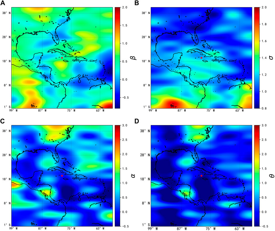
FIGURE 1. Construction process of the C-value perturbation amplitude matrix θ within ± 20° of the epicenter of the Mw7.7 earthquake off southern Cuba. (A) Matrix of background field averages constructed from C values from 70 to 40 days before the earthquake β; (B) Matrix of standard variance values σ of the background field constructed from the C-values from 70 to 40 days before the earthquake; (C) The mean matrix α constructed from the C-values from 45 to 35 days before the earthquake; (D) The resulting matrix θ calculated according to Eq. 4.

The perturbation amplitude θ concerning the background field is calculated (Figure 1D). Eq. 4 represents the multiple of the deviation of the C value calculated by Eq. 3 from its standard variance concerning the background field, i.e., the perturbation amplitude for the background field.

From the construction of the background field observation model and the extraction process of the disturbance amplitude in Figure 1, we can see that: the background field intensity is relatively calm except for the lower right corner, which is far from the epicenter, where the highest value exceeds 2.0, and the variation range is between −0.6 and 1.0; the standard variance matrix of the background field is between 0.5 and 1.4, except for the highest value near the equator, which reaches 1.8; the matrix α of the inception zone is relatively calm between −0.5 and 2.0 the period from 40 to 35 days before the earthquake, and the overall disturbance amplitude σ ranges from 0.5 to 1.0, which is relatively calm and reliable.

3.3 Statistical overlay method

The maximum perturbation amplitude ${\left|\left\{{\theta }_{\left(n,t\right)}\right\}\right|}_{\mathit{max}}$ for each satellite cycle of a single earthquake case is calculated using the above method, where n represents the different vibration cases (n = 1, 2, 3, ......, n), t represents different periods in the same earthquake case (t = −7, −6, −5, ......, 1), Then, the ${\left|\left\{{\theta }_{\left(n,t\right)}\right\}\right|}_{\mathit{max}}$ of each case is summed up and divided by the number of cases n to obtain the final result θ_fin.

${\theta }_{fin}=\frac{1}{n}{{\displaystyle \sum }_{i=0}^n\left|\left\{{\theta }_{\left(n,t\right)}\right\}\right|}_{\max }(5)$

3.4 Results of earthquake analysis in Cuban waters

According to the above method, in this study, the C values were obtained by processing the spatial electric field before and after the earthquake in the southern sea of Cuba. Then their spatial and temporal characteristics were analyzed. Forty days before and 5 days after the earthquake (21 December 2019–3 February 2020) were selected as the study period. The period was divided into nine time periods with a five-day cycle. The observed model β and σ of the C value background field ±20° above the epicenter and the corresponding α matrix were calculated for each time period. The corresponding θ matrix was obtained using Eq. 4, and the results are shown in Figure 2.

FIGURE 2

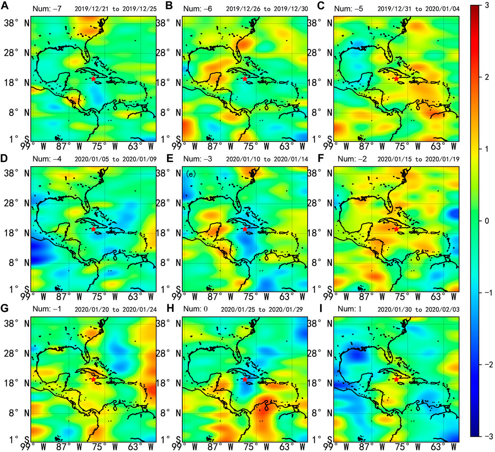
FIGURE 2. Spatial and temporal evolution characteristics of theta values before and after the 2020 earthquake in the southern waters of Cuba. (Num: −7 to Num: −1 represents the seventh cycle to the first cycle before the earthquake, Num: 0 is the period of earthquake, Num: 0 is the first period after the earthquake. Num: −7 to Num: 2 corresponds to (A–I).

Figure 2 gives the spatial and temporal evolution characteristics of the C values over the earthquake in the southern sea of Cuba from 21 December 2019, to 3 February 2020, relative to the background field observation model. In Figures 2A, B, we can see that the C value perturbations are relatively stable from 40 to 30 days before the earthquake, and the θ values are stable from −1.0 to 1.5 without large perturbations; in Figure 2C, we can see that the θ perturbations have increased and are positively correlated; in Figures 2D, E, the perturbations are large and exceed 2.0σ; in Figures 2F, G show that the theta value in the center of the earthquake preparation zones is the most significant relative to this period from 15 to 5 days before the earthquake, and the magnitude of the disturbance is gradually increasing; Figure 2H represents the pro-seismic cycle (4 days before the earthquake and the day of the earthquake), and the theta value at the epicenter is negatively correlated for other areas. The strong disturbance in the southeastern part of the epicenter reaches 2.1σ, and the magnitude reaches the maximum within 45 days; in Figure 2H, we can see a negative correlation with the magnitude of the disturbance in the epicenter. The same negative disorder is also observed in Figures 2D, E, but the phenomenon is not as pronounced as in Figure 2H, which may be caused by the magnitude 6 and 6. Five earthquakes on 7 January and 11 January 2020. Figure 2I shows that the maximum θ value reaches 1.6σ only 5 days after the earthquake.

4 Statistical research

The process of earthquake incubation is a highly complex physicochemical evolution process. The medium in which earthquakes occur and propagate is different, so the anomalous perturbations in the space ionosphere caused by earthquakes are also complicated and diverse, and the anomalous phenomena extracted from only a single earthquake cannot be rigorously verified to obtain the objective law of electric field perturbations in the ionosphere caused by earthquakes. Therefore, in this paper, we will use the ionospheric electric field data observed by the CSES during 2019–2021 and process the data recorded by the United States Geological Survey (USGS.gov | Science for a changing world) during this period using the above method, a comparative analysis of all the seismic cases studied in this paper was first carried out with and without the influence of magnetic storms; Then, the correlation between different characteristics of earthquakes and the anomalous disturbance of electric field is analyzed from the perspective of the spatial and temporal distribution of the ionospheric electric field disturbance, to obtain the common performance of different characteristics of earthquakes in spatial and temporal distribution.

In this study, Figure 3 contains 15 shock cases with M_S ≥ 7.0 and 170 cases with 6.0 ≤ M_S ≤ 7.0.

FIGURE 3

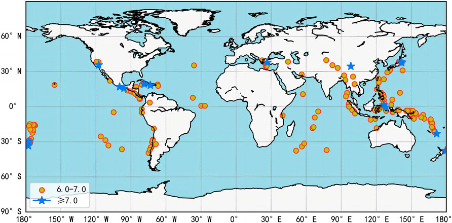
FIGURE 3. Global distribution of partial earthquake cases in 2019–2021. The x-axis is the geographic longitude, and the y-axis is the geographic longitude.

4.1 Different earthquake magnitude

According to previous studies, the energy released by an earthquake varies with its magnitude. The larger the magnitude, the greater the energy released, resulting in a broader range of anomalous spatial electric field disturbances and more pronounced anomalies. Therefore, the target earthquake cases are divided into two categories: one is of magnitude 6–7, and the other is of magnitude seven or higher. Then, we divided the study area into northern and southern hemispheres and performed spatial and temporal analyses for the two types of earthquakes (Xiong et al., 1999; Zhou et al., 2017). The comparison results are shown in Figures 4, 5.

FIGURE 4

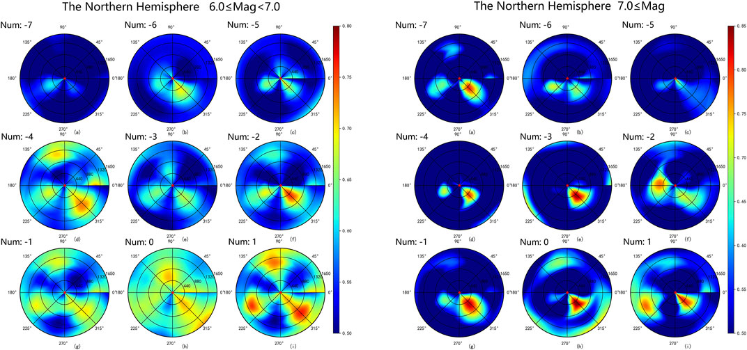
FIGURE 4. Spatial and temporal distribution of spatial electric field ELF band disturbances for earthquakes of magnitude 6.0–7.0 and magnitude 7+ in the Northern Hemisphere. (Num: −7 to Num: −1 represents the seventh cycle to the first cycle before the earthquake, Num: 0 is the period of earthquake, Num: 0 is the first period after the earthquake).

FIGURE 5

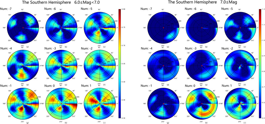
FIGURE 5. Spatial and temporal distribution of spatial electric field ELF band perturbations of magnitude 6.0–7.0 and magnitude 7+ earthquakes in the Southern Hemisphere. (Num: −7 to Num: −1 represents the seventh cycle to the first cycle before the earthquake, Num: 0 is the period of earthquake, Num: 0 is the first period after the earthquake).

The examples of earthquakes of different magnitudes in the northern hemisphere are shown in Figure 4 (81 earthquakes, including ten earthquakes of magnitude seven or higher and 71 earthquakes of magnitude 6.0–7.0), which are spatially and temporally analyzed. Observe the left graph to get, For earthquakes with magnitudes ranging from 6.0 to 7.0 in the Northern Hemisphere, the numerical fluctuate between 0.50 and 0.8 in the entire earthquake preparation zones, and are quiet for 40 to 25 days before the earthquake; from the 34th day before the earthquake, the values started to rise within 880 km South of the epicenter; the anomalies in the entire earthquake preparation zones began to rise during the 24–20 days before the earthquake, and weakened significantly during the 19–15 days before the earthquake, but were still more potent than the 40–25 days before the earthquake; from 14 days before the earthquake, the values in the area within 880 km southeast of the epicenter increased and were close to the maximum value of 8.0 for the whole earthquake preparation period, and the values in the entire earthquake preparation zones increased until the pro-seismic cycle, and the values in most of the earthquake preparation zones reached 0.65 or more during the pre-seismic process; the values started to decrease in some areas after the earthquake, but some areas showed an increase. Observe the graph on the right, to get. For earthquakes of magnitude 7.0 or higher in the Northern Hemisphere, the numerical range of the entire earthquake preparation zone fluctuates between 0.50 and 0.85. The pre-earthquake period of 19 to 15 days and the pre-earthquake period are significantly different from other periods; in these two time periods, the higher values in the southwest of the epicenter disappeared, and anomalous areas appeared in the southeast of the pre-seismic cycle at the edge of the earthquake preparation zones. Comparing earthquakes of magnitude seven or higher with those of magnitude 6.0–7.0, we can see that the maximum values of the range of magnitude seven or higher are higher, and the disturbances are more prominent.

The examples of earthquakes of different magnitudes in the Southern hemisphere are shown in Figure 5 (104 earthquakes, including five earthquakes of magnitude seven or higher and 99 earthquakes of magnitude 6.0–7.0), which are spatially and temporally analyzed. Observe the left graph to get, for earthquakes with magnitudes ranging from 6.0 to 7.0 in the Southern Hemisphere, the numerical fluctuate between 0.50 and 0.8 in the entire earthquake preparation zones; there are three numerical anomalies in the earthquake preparation zones during the whole earthquake preparation period, with the epicenter northwest, northeast, and southwestward offset by 5°; from 40 to 30 days before the earthquake, the anomalies were relatively low and negligible compared to other periods, and there were few anomalies within 440 km of the epicenter; from the 29th day before the earthquake, the range of anomalous areas increased, and the abnormal values in some areas increased; the anomalous values in the southern part of the region reached the highest value of 8.0 the 9–5 days before the earthquake; during the pre-seismic cycle, the values are high in most areas of the earthquake preparation zones; after the earthquake, the values start to decrease in some areas. Observe the graph on the right to get for earthquakes of magnitude 7.0 or higher in the Southern Hemisphere, the numerical range of the entire earthquake preparation zones fluctuates between 0.50 and 1.10 and is generally quiet from 40 to 30 days before the earthquake; the abnormal area in the epicenter gradually expanded and strengthened from the 29th day before the earthquake until the day of the earthquake; at the time of pre-seismic cycle, The maximum anomaly value of 1.1 is reached at the pre-seismic period, and the anomaly range is the largest; after the earthquake, the anomalies began to decrease, and the range was reduced. As in the northern hemisphere, the maximum value of the magnitude seven and above range is higher, and the disturbance is more prominent.

4.2 Different regional types of earthquakes

Previous studies have shown that the medium and magnetic field affect the propagation of electromagnetic signals during the upward propagation from the earthquake source during the earthquake preparation period and that the influence of the Earth’s rotation produces different deviations of electromagnetic signals in the northern and southern hemispheres. Therefore, in this paper, we first divided the seismic events into two regions by latitude in the North and southern hemispheres and then counted the sea and land earthquakes separately. The statistical results are shown in Figures 6, 7.

FIGURE 6

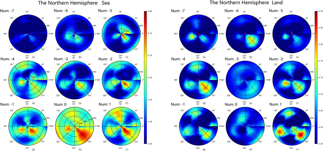
FIGURE 6. Spatial and temporal distribution of pre-seismic disturbances in the ELF frequency band (19.5–250 Hz) of the space electric field obtained from sea and land earthquakes of magnitude 6.0 or higher in the Northern Hemisphere. (Num: −7 to Num: −1 represents the seventh cycle to the first cycle before the earthquake, Num: 0 is the period of earthquake, Num: 0 is the first period after the earthquake).

FIGURE 7

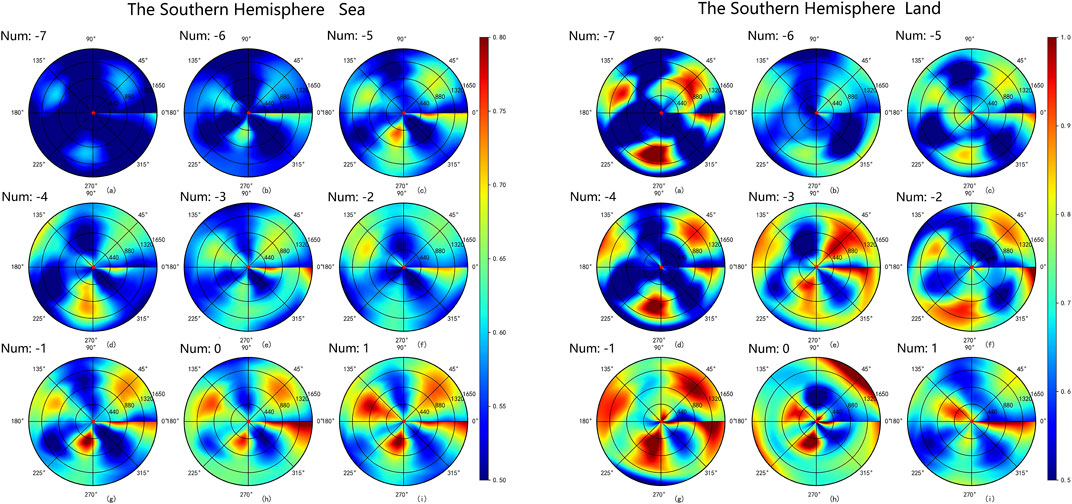
FIGURE 7. Spatial and temporal distribution of spatial electric field ELF band (19.5–250 Hz) perturbations in sea and land earthquakes above magnitude 6.0 in the Southern Hemisphere. (Num: −7 to Num: −1 represents the seventh cycle to the first cycle before the earthquake, Num: 0 is the period of earthquake, Num: 0 is the first period after the earthquake).

The spatial and temporal analysis of the earthquake cases of magnitude 6.0 or higher in the northern hemisphere (81 earthquakes, including 52 marine earthquakes and 29 land earthquakes) in Figure 6, the left panel shows that the values fluctuate between 0.50 and 0.80 during the earthquake preparation period in the northern hemisphere region; the space weather was stable 40–30 days before the earthquake, the anomalous values in the southeast area within 440 km from the epicenter were higher from 29 to 25 days before the earthquake and reached the highest value in the whole earthquake preparation zones; the maximum value of the time period decreases between 24 and 20 days before the earthquake, but the value increases in the entire range of the earthquake preparation zones during this time period, and most of the values in the southeast area are above 0.65; The range of anomalies in earthquake preparation zones narrowed during the period from 19 to 15 days before the earthquake, but the maximum value in the southeastern region started to increase compared with that in the period from 24 to 20 days before the earthquake; The maximum value in the southeast region began to rise from 14 to 10 days before the earthquake, and the influence area started to spread to the southeast. The maximum value of the epicentral range reached 0.75 at the time of the pre-seismic cycle (the fourth day before the earthquake to the day of the earthquake). Still, most of the values in the southeastern region were above 0.7 relative to the time range of 29 to 25 days before the earthquake, and the anomalous range was much more extensive than that of 29 to 25 days before the earthquake; the values of the pre-seismic period are generally high in the whole inception area, and most of them are above 0.60; the anomalous range decreases after the earthquake. In the right panel, we can see that the fluctuation range of the values in the northern hemisphere land earthquakes is between 0.50 and 0.90. In the earthquake preparation zones, except for the 19–15 days before the earthquake and earthquake preparation zones, there are high values in the southwest, southeast, and northwest directions of the earthquake preparation zones, and the other areas are generally calm. In the 19–15 days before the earthquake and during the pre-seismic cycle, the range of values in the entire earthquake preparation zones is high, which is significantly different from other periods.

The spatial and temporal analyses of the earthquake cases of magnitude 6.0 and above in the southern hemisphere (104 earthquakes of different origins, including 94 marine earthquakes and 10 land earthquakes) are shown in Figure 7. Observe the left graph to get, the numerical range of the earthquake preparation zones fluctuates from 0.50 to 0.8 during the earthquake preparation period in the northern hemisphere region, 40–30 days before the earthquake is relatively calm; From 29 days before the earthquake, the values in the earthquake preparation zones started to increase as a whole, and during the period from 24 to 20 days before the earthquake, the values within 440 km of the epicenter began to grow, and most of the areas south of the epicenter had values greater than 0.65, spreading from the epicenter to the northeast to the edge of the geostrophic zone; from 9 days before to 5 days after the earthquake, a region of high values appeared to the southwest of the epicenter, and a significant increase in values was observed within 440 km of the epicenter during the pre-seismic cycle; during the whole earthquake preparation period, although there is an area North of the epicenter with values ranging from 0.65 to 0.80, the overall values are high, but the anomalous high values in the earthquake preparation zones spread to the South.

In the southern hemisphere land earthquakes, the anomalies in the earthquake preparation zones are high from 40 to 30 days before the earthquake, but the values are low within 440 km of the epicenter. The overall values within 400 km of the epicenter increased in the time range of 29 to 25 days before the earthquake; The phenomenon from 40 to 35 days before the earthquake was similar to that from 29 to 25 days before the earthquake, and although a high anomaly area was observed in the earthquake preparation zones, it was quiet within 440 km of the epicenter; From 9 days before the earthquake to the day of the earthquake, most of the values in the area south of the epicenter reached 0.9 or higher. The values in the earthquake preparation zones were higher than those in other periods. The overall importance of the post-earthquake earthquake preparation zones started to decrease.

4.3 Comparative analysis of earthquake cases affected by magnetic storms and those not affected by magnetic storms

To explore the influence of magnetic storms on the analysis results, this paper first disregards that the ZH-1 satellite will be affected by magnetic storms during the observation, adopts the method in Chapter 3 to process its data, and then performs statistical analysis on the processing results, and compares the statistical results of the seismic case study when the data affected by magnetic storms are removed, as shown in Figure 8.

FIGURE 8

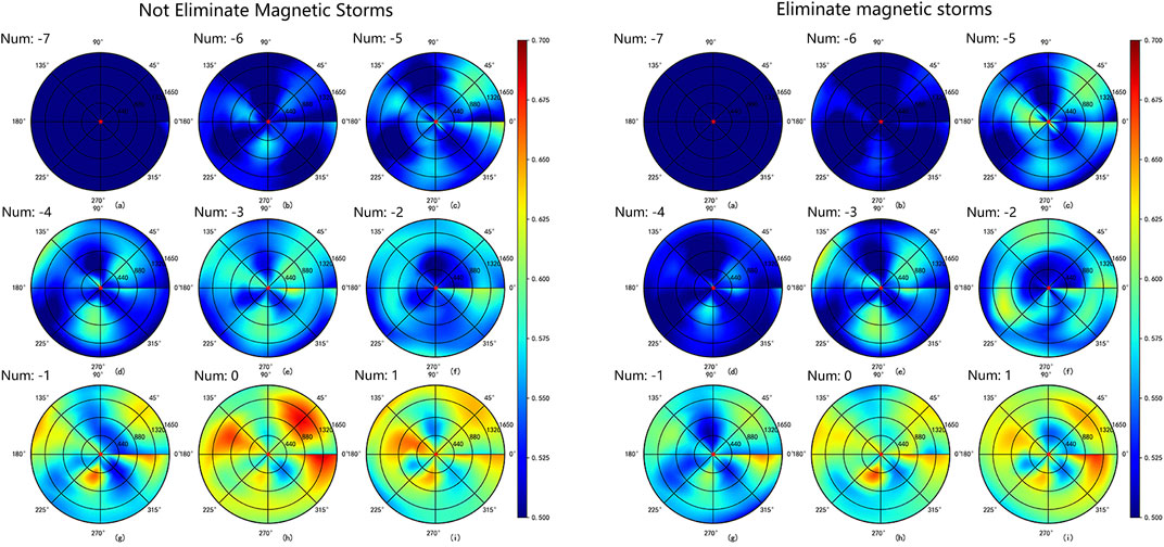
FIGURE 8. Spatial and temporal distribution of pre-seismic disturbances in the ELF frequency band (19.5–250 Hz) of the spatial electric field after excluding the effects of magnetic storms for global magnitude 6.0 or higher earthquakes and without excluding the effects of magnetic storms. (Num: −7 to Num: −1 represents the seventh cycle to the first cycle before the earthquake, Num: 0 is the period of earthquake, Num: 0 is the first period after the earthquake).

The Spatio-temporal analysis of the global earthquake cases of magnitude 6.0 or higher (185 cases) in Figure 8, the left panel shows the results of the statistical analysis without excluding the orbital data with Kp > 3, and the right panel shows the results of the investigation without excluding the orbital data with Kp > 3. The comparison indicates that the anomalies in both the left and right panels are more evident in the pre-seismic cycle. Still, the anomalies in the left panel are much more than those in the right. The decreasing trend of numerical intensity within 880 km of the epicenter in the first post-earthquake cycle needs to be clarified. In the right panel, the anomalies spread to the outer part of the earthquake preparation zones, and the intensity of the anomalies decreases significantly within 880 km of the epicenter in the first post-earthquake period. The results indicate that magnetic storms can affect the observation results of the CSES satellite and interfere with the extraction of ionospheric electric field anomalies before the earthquake by the CSES.

4.4 Comparison analysis of random and real earthquakes

To investigate the correlation between earthquakes and ELF band perturbations, we compare the spatial and temporal evolution of the ELF band (19.5–250 Hz) observed by the CSES during random earthquakes in calm weather conditions and without strong earthquakes using the same data processing method. The random earthquakes were selected as follows: random earthquakes occurred between January 2019 and December 2021, and there were no earthquakes of magnitude 7.0 or higher in the first 2 months to the last 10 days of the time point. Then, each random earthquake’s location corresponds to the actual earthquake’s place, and finally, the unexpected earthquake is processed using the above method. The statistical results of the random earthquakes are shown in Figure 9.

FIGURE 9

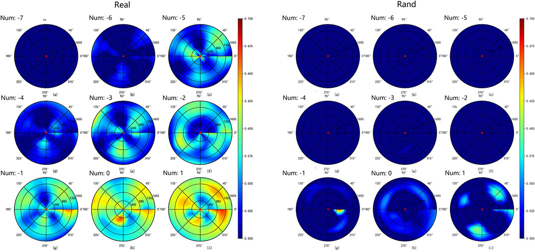
FIGURE 9. Spatial electric field ELF frequency band (19.5–250 Hz) pre-seismic disturbance spatial and temporal distribution of real and random earthquakes. (Num: −7 to Num: −1 represents the seventh cycle to the first cycle before the earthquake, Num: 0 is the period of earthquake, Num: 0 is the first period after the earthquake).

The Spatio-temporal analysis of the real earthquake cases (185 cases) and the random earthquake cases (185 cases) in Figure 9, the left panel shows the spatio-temporal distribution of the real earthquake and the right panel shows the spatio-temporal distribution of the random earthquake. For comparison, the overall values are between 0.50 and 0.70 for pregnant earthquakes and 0.50 and 0.60 for random earthquakes; The disturbances of real earthquakes appear, spread, and then disappear in the pregnant seismic zone in a relatively regular manner, although the high-intensity anomalies do not occur within the epicenter region, their anomalous areas are all spread out from the epicenter; Only a small anomalous region appears in the first period before the earthquake, and the anomaly is obviously independent of the epicenter; then there is no obvious correlation between the random earthquake and the ELF band (19.5–250 Hz) perturbation of the space electric field.

Although spatial anomalies such as strong earthquakes and magnetic storms are avoided in the time and space of the selected random earthquakes, these influences cannot be avoided entirely, thus causing weak perturbations in the ionosphere. Still, these perturbations occur in the periphery of the earthquake preparation zones, and no significant changes in the pre-earthquake anomalies are observed in the spatial and temporal range. The comparison results significantly correlate the ELF frequency band (19.5–250 Hz) disturbances and natural earthquakes.

5 Discussion and conclusion

5.1 Discussion

The statistical results of this paper show that the overall values of the pre-seismic period (4 days before the earthquake and the day of the earthquake) are higher than those of the other periods in the comparative study of different earthquake magnitudes in the range of magnitude 6.0–7.0, however, the anomalies in other periods are mainly concentrated within 880 km, but the anomalous disturbances are less noticeable. For earthquakes of magnitude 7 or higher, the main abnormalities were also found to occur during the pre-seismic cycle, and the anomalies are relative to the results of the 6.0–7.0 magnitude earthquake analysis, and the maximum values of the anomalies were higher than those for earthquakes of magnitude 6.0 to 7.0.

Comparing sea and land earthquakes, sea seismic anomalies are more easily observed in the northern hemisphere. In the Southern Hemisphere, land seismic anomalies are more evident than sea seismic anomalies. It is possible that there are only ten earthquake cases in the Southern Hemisphere during the study period, while there are 94 sea earthquakes in the Southern Hemisphere, and the sample gap is too large to form a stable conclusion.

In the analysis of earthquake cases, different degrees of anomalous disturbances were also observed in the post-earthquake period. The most noticeable results were found in the case of marine earthquakes and 6.0–7.0 magnitude earthquakes. This may be because the tectonic plates are still colliding with each other after the mainshock, or secondary hazards such as tsunamis and volcanic eruptions may also cause ionospheric disturbances after the earthquake. Earthquakes are generated by the collision and compression of tectonic plates, and the recovery of the crust may cause ionospheric disturbances after the earthquake due to the displacement and faulting caused by the earthquake. The energy released from 6.0 to 7.0 magnitude earthquakes is small and not as much as that from 7.0 magnitude earthquakes, so the resistance to disturbance is lower than that of 7.0 magnitude earthquakes and above. This is not analyzed in depth in this paper, and further research is needed.

According to previous studies, electromagnetic radiation is shifted southward in the northern hemisphere and northward in the southern hemisphere due to the equatorial influence. Still, in this study, the opposite situation occurs. Some anomalies appear North of the northern hemisphere case study and South of the epicenter in the southern hemisphere case study. However, this phenomenon always disappears when the anomalies are most pronounced during the earthquake preparation period, and the overall results are consistent with previous studies. Therefore, this paper does not investigate this phenomenon in depth, and further research is needed to determine whether this phenomenon is related to earthquakes.

5.2 Conclusion

In this paper, we analyze the ELF (19.5–250 Hz) data in the space electric field band observed by the CSES from 2019 to 2021 and study the spatial and temporal distribution characteristics of 185 cases of earthquakes of magnitude 6.0 or higher, according to the location and extent of the earthquakes, and obtain the following four conclusions.

• By dividing the northern and southern hemispheres, we found that the significant anomalous disturbances in the northern hemisphere are shifted to the South, and the southern hemisphere is shifted to the North during earthquakes.

• From the spatial and temporal statistics, the first pre-seismic disturbance occurs 29 to 25 days before the earthquake in the sea area. Then the volume release diffusion occurs 29 to 20 days before the earthquake, reaching the most obvious seismic disturbance in the pre-seismic cycle. The first anomaly in the northern hemisphere land earthquakes occurs 19–15 days before the earthquake and is most pronounced during the pre-seismic cycle.

• Pre-earthquake anomalies are more easily observed in marine earthquakes than inland earthquakes.

• With the increase in earthquake magnitude, the intensity of ionospheric anomalies caused by earthquakes of magnitude seven or higher is significantly higher than that of earthquakes of magnitude 6–7, and the resistance to disturbance is higher than that of earthquakes of magnitude 6–7, making the anomalies most easily observed.

Data availability statement

The original contributions presented in the study are included in the article/supplementary material, further inquiries can be directed to the corresponding authors.

Author contributions

F-ZZ was mainly responsible for the experimental part and writing of the paper; J-PH and ZL was mainly responsible for the experimental data compilation and revision of the paper; X-HS provided guidance and comments on the main experiments of the paper, and others were responsible for reviewing and supervising the quality and content of the paper. All authors read and approved the final manuscript.

Funding

This study was jointly funded by National Natural Science Foundation of China (NSFC) Project No. 42104159, National Key Research and Development Program of China Project no. 2018YFC1503501, the Asia-Pacific Space Cooperation Organization earthquake special project phase 2, ISSI-BJ2019, Dragon 5 Cooperation Proposal, #58892, #59308.

Acknowledgments

This work made use of the data from the CSES mission, a project funded by the China National Space Administration (CNSA) and the China Earthquake Administration (CEA). The data could be available from www.leos.ac.cn. We thank Professor Xuemin Zhang of the Institute of Earthquake Prediction, China Earthquake Administration, for her guidance and comments during the research process of the paper, and thank Bojing Zhu of Yunnan Observatories, CAS for the English. We thank the editors and reviewers for their suggestions and hard work.

Conflict of interest

The authors declare that the research was conducted in the absence of any commercial or financial relationships that could be construed as a potential conflict of interest.

Publisher’s note

All claims expressed in this article are solely those of the authors and do not necessarily represent those of their affiliated organizations, or those of the publisher, the editors and the reviewers. Any product that may be evaluated in this article, or claim that may be made by its manufacturer, is not guaranteed or endorsed by the publisher.

References

Akhoondzadeh, M., De Santis, A., Marchetti, D., and Shen, X. (2022). Swarm-TEC satellite measurements as a potential earthquake precursor together with other Swarm and CSES data: The case of Mw7.6 2019 Papua New Guinea seismic event. Front. Earth Sci. 10. doi:10.3389/feart.2022.820189

CrossRef Full Text | Google Scholar

Ampferer, M., Denisenko, V., Hausleitner, W., Krauss, S., Stangl, G., Boudjada, M. Y., et al. (2010). Decrease of the electric field penetration into the ionosphere due to low conductivity at the near ground atmospheric layer. Ann. Geophys. 28, 779–787. doi:10.5194/angeo-28-779-2010

CrossRef Full Text | Google Scholar

Ambrosi, G., Bartocci, S., Basara, L., Battiston, R., Burger, W. J., Carfora, L., et al. (2018). The HEPD particle detector of the CSES satellite mission for investigating seismo-associated perturbations of the Van Allen belts. Science China Technological Sciences 61, 643–652

CrossRef Full Text | Google Scholar

Berthelier, J. J., Godefroy, M., Leblanc, F., Malingre, M., Menvielle, M., Lagoutte, D., et al. (2006). ICE, the electric field experiment on DEMETER. Planet. Space Sci. 54, 456–471. doi:10.1016/j.pss.2005.10.016

CrossRef Full Text | Google Scholar

Cao, J., Zeng, L., Zhan, F., Wang, Z., Wang, Y., Chen, Y., et al. (2018). The electromagnetic wave experiment for CSES mission: Search coil magnetometer. Sci. China Technol. Sci. 61, 653–658. doi:10.1007/s11431-018-9241-7

CrossRef Full Text | Google Scholar

Diego, P., Huang, J., Piersanti, M., Badoni, D., Zeren, Z., Yan, R., et al. (2020). The electric field detector on board the China seismo electromagnetic satellite—in-orbit results and validation. Instruments 5 (1), 1. doi:10.3390/instruments5010001

CrossRef Full Text | Google Scholar

Dobrovolsky, I. P., Zubkov, S. I., and Miachkin, V. I. (1979). Estimation of the size of earthquake preparation zones. pure Appl. Geophys. 117, 1025–1044. doi:10.1007/bf00876083

CrossRef Full Text | Google Scholar

Gao, Y., Chen, X., Hu, H., Wen, J., Tang, J., and Fang, G. (2014). Induced electromagnetic field by seismic waves in Earth's magnetic field. J. Geophys. Res. Solid Earth 119, 5651–5685. doi:10.1002/2014jb010962

CrossRef Full Text | Google Scholar

Gokhberg, M. B., Morgounov, V. A., Yoshino, T., and Tomizawa, I. (1982). Experimental measurement of electromagnetic emissions possibly related to earthquakes in Japan. J. Geophys. Res. 87, 7824–7828. doi:10.1029/jb087ib09p07824

CrossRef Full Text | Google Scholar

Grimalsky, V. V., Hayakawa, M., Ivchenko, V. N., Rapoport, Y. G., and Zadorozhnii, V. I. (2003). Penetration of an electrostatic field from the lithosphere into the ionosphere and its effect on the D-region before earthquakes. J. Atmos. Solar-Terrestrial Phys. 65, 391–407. doi:10.1016/s1364-6826(02)00341-3

CrossRef Full Text | Google Scholar

Hayakawa, M., Ito, T., and Smirnova, N. A. (1999). Fractal analysis of ULF geomagnetic data associated with the Guam Earthquake on August 8, 1993. Geophys. Res. Lett. 26, 2797–2800. doi:10.1029/1999gl005367

CrossRef Full Text | Google Scholar

He, Y. (2020). Study on seismo-ionospheric phenomena based on electric density data record by Swarm and DEMETER satellite. Doctoral thesis. Beijing, (China): Institute of Geophysics, China Earthquake Adminstration (in Chinese).

Google Scholar

Hu, Y., Zeren, Z. M., Huang, J., Zhao, S., Guo, F., Wang, Q., et al. (2020). Algorithms and implementation of wave vector analysis tool for the electromagnetic waves recorded by the CSES satellite. Chin. J. Geophys. 63 (5), 1751–1765. doi:10.6038/cjg2020N0405

CrossRef Full Text | Google Scholar

Huang, H., Yan, R., Liu, D., Xu, S., Lin, J., Guo, F., et al. (2021). The variations of plasma density recorded by CSES-1 satellite possibly related to Mexico Ms 7.1 earthquake on 8th September 2021. Natural Hazards Research 2 (1), 11–16.

Google Scholar

Huang, J., Jia, J., Yin, H., Li, Z., Li, J., Shen, X., et al. (2022). Study of the statistical characteristics of artificial source signals based on the CSES. Front. Earth Sci. 10. doi:10.3389/feart.2022.883836

CrossRef Full Text | Google Scholar

Huang, J., Lei, J., Li, S., Zeren, Z., Li, C., Zhu, X., et al. (2018). The Electric Field Detector (EFD) onboard the ZH-1 satellite and first observational results. Earth Planet. Phys. 2, 469–478. doi:10.26464/epp2018045

CrossRef Full Text | Google Scholar

Huang, J., Liu, J., Ouyang, X., and Li, W. (2011). Analysis of the energetic particles around the chili earthquake of m8. 8. Earthq. Res. China 25 (002), 166–172.

Google Scholar

Huang, Q. (2002). One possible generation mechanism of co-seismic electric signals. Proc. Jpn. Acad. Ser. B 78, 173–178. doi:10.2183/pjab.78.173

CrossRef Full Text | Google Scholar

Johnston, M, J, S. (1997). Review of electric and magnetic fields accompanying seismic and volcanic activity. Surv. Geophys 18, 441–476. doi:10.1023/a:1006500408086

CrossRef Full Text | Google Scholar

Li, M., Shen, X., Parrot, M., Zhang, X., Zhang, Y., Yu, C., et al. (2020). Primary joint statistical seismic influence on ionospheric parameters recorded by the CSES and DEMETER satellites. J. Geophys. Res. Space Phys. 125 (1). doi:10.1029/2020ja028116

CrossRef Full Text | Google Scholar

Li, Z., Li, J., Huang, J., Yin, H., and Jia, J. (2022a). Research on pre-seismic feature recognition of spatial electric field data recorded by CSES. Atmosphere 13, 179. doi:10.3390/atmos13020179

CrossRef Full Text | Google Scholar

Li, Z., Yang, B., Huang, J., Yin, H., Yang, X., Liu, H., et al. (2022b). Analysis of pre-earthquake space electric field disturbance observed by CSES. Atmosphere 13 (6), 934. doi:10.3390/atmos13060934

CrossRef Full Text | Google Scholar

Lin, J., Shen, X., Hu, L., Wang, L., and Zhu, F. (2018). CSES GNSS ionospheric inversion technique, validation and error analysis. Sci. China Technol. Sci. 61, 669–677. doi:10.1007/s11431-018-9245-6

CrossRef Full Text | Google Scholar

Liu, J. Y., Chen, C., Chen, Y., Yang, W., Oyama, K., and Kuo, K. (2010). A statistical study of ionospheric earthquake precursors monitored by using equatorial ionization anomaly of GPS TEC in Taiwan during 2001-2007. J. Asian Earth Sci. 39, 76–80. doi:10.1016/j.jseaes.2010.02.012

CrossRef Full Text | Google Scholar

Marchetti, D., De Santis, A., Shen, X., Campuzano, S. A., Perrone, L., Piscini, A., et al. (2020). Possible Lithosphere-Atmosphere-Ionosphere Coupling effects prior to the 2018 Mw = 7.5 Indonesia earthquake from seismic, atmospheric and ionospheric data. J. Asian Earth Sci. 188, 104097. doi:10.1016/j.jseaes.2019.104097

CrossRef Full Text | Google Scholar

Nepeina, K. S. (2021). The capabilities of analyzing the seismo-electromagnetic satellite CSES-01 data for monitoring of seismic activity of the Northern Tien Shan. IOP Conf. Ser. Earth Environ. Sci. 929, 012017. doi:10.1088/1755-1315/929/1/012017

CrossRef Full Text | Google Scholar

Ouyang, X., Bortnik, J., Ren, J., and Berthelier, J. J. (2019). Features of nightside ULF wave activity in the ionosphere. J. Geophys. Res. Space Phys. 124, 9203–9213. doi:10.1029/2019ja027103

CrossRef Full Text | Google Scholar

Ouzounov, D., and Freund, F. (2004). Mid-infrared emission prior to strong earthquakes analyzed by remote sensing data. Adv. Space Res. 33, 268–273. doi:10.1016/s0273-1177(03)00486-1

CrossRef Full Text | Google Scholar

Ouzounov, D., Liu, D., Chun-li, K., Cervone, G., Kafatos, M. C., and Taylor, P. T. (2007). Outgoing long wave radiation variability from IR satellite data prior to major earthquakes. Tectonophysics 431, 211–220. doi:10.1016/j.tecto.2006.05.042

CrossRef Full Text | Google Scholar

Ouzounov, D., and Yagodin, A. (2021). Progress in the short-term earthquake forecasting by integrating KaY wave analysis and satellite observations. doi:10.48550/arXiv.2105.08570

CrossRef Full Text | Google Scholar

Park, C. G., and Dejnakarintra, M. (1973). Penetration of thundercloud electric fields into the ionosphere and magnetosphere: 1. Middle and subauroral latitudes. J. Geophys. Res. 78, 6623–6633. doi:10.1029/ja078i028p06623

CrossRef Full Text | Google Scholar

Parrot, M., Benoist, D. M., Berthelier, J. J., Blecki, J., Chapuis, Y., Colin, F., et al. (2006). The magnetic field experiment IMSC and its data processing onboard DEMETER: Scientific objectives, description and first results. Planet. Space Sci. 54, 441–455. doi:10.1016/j.pss.2005.10.015

CrossRef Full Text | Google Scholar

Parrot, M. (2011). Statistical analysis of the ion density measured by the satellite DEMETER in relation with the seismic activity. Earthq. Sci. 24, 513–521. doi:10.1007/s11589-011-0813-3

CrossRef Full Text | Google Scholar

Piersanti, M., Materassi, M., Battiston, R., Carbone, V., Cicone, A., D’Angelo, G., et al. (2020). Magnetospheric-ionospheric-lithospheric coupling model. 1 observations during the 5 August 2018 bayan earthquake. Remote. Sens. 12, 3299. doi:10.3390/rs12203299

CrossRef Full Text | Google Scholar

Pulinets, S. A., and Boyarchuk, K. A. (2004). Ionospheric precursors of earthquakes. New York: Springer, 174–195.

Google Scholar

Pulinets, S. A., Ouzounov, D., and Hattori, K. (2018). Pre-earthquake processes: A multidisciplinary approach to earthquake prediction studies. New Jersey, NJ: Wiley Geology & Geophysics

Google Scholar

Pulinets, S. A., Ouzounov, D., Karelin, A. V., and Davidenko, D. (2015). Physical bases of the generation of short-term earthquake precursors: A complex model of ionization-induced geophysical processes in the lithosphere-atmosphere-ionosphere-magnetosphere system. Geomagnetism Aeronomy 55, 521–538. doi:10.1134/s0016793215040131

CrossRef Full Text | Google Scholar

Qian, G., Zeren, Z. M., Zhang, X, M., and Shen, X. (2016). Spatio-temporal evolution of electromagnetic field pre-and post-earthquakes. Acta Seismol. Sin. 38 (2), 259–271. doi:10.11939/jass.2016.02.010

CrossRef Full Text | Google Scholar

Scotti, V., and Osteria, G. (2019). The HEPD detector on board CSES satellite: In-flight performance. Nucl. Part. Phys. Proc. 936, 92–97. doi:10.1016/j.nuclphysbps.2019.07.014

CrossRef Full Text | Google Scholar

Shen, X., Zhang, X., Yuan, S., Wang, L., Cao, J., Huang, J., et al. (2018). The state-of-the-art of the China Seismo-Electromagnetic Satellite mission. Sci. China Technol. Sci. 61, 634–642. doi:10.1007/s11431-018-9242-0

CrossRef Full Text | Google Scholar

Sorokin, V. M., Chmyrev, V. M., and Hayakawa, M. (2015). Electrodynamic coupling of lithosphere--atmosphere--ionosphere of the earth. New York, NY: Nova Science Press

Google Scholar

Wang, Z., Zhou, C., Zhao, S., Xu, X., Liu, M., Liu, Y., et al. (2021). Numerical study of global ELF electromagnetic wave propagation with respect to lithosphere-atmosphere-ionosphere coupling. Remote. Sens. 13, 4107. doi:10.3390/rs13204107

CrossRef Full Text | Google Scholar

Xiong, N, L., Tang, C, C., and Li, X, J. (1999). Introduction to ionospheric physics. Wuhan: Wuhan University Press.

Google Scholar

Yang, Y., Zhima, Z., Shen, X., Chu, W., Huang, J., Wang, Q., et al. (2020). The first intense geomagnetic storm event recorded by the China seismo-electromagnetic satellite. Space weather. 18 (1). doi:10.1029/2019sw002243

CrossRef Full Text | Google Scholar

Zeren, Z, M., Shen, X., Cao, J., Zhang, X., Huang, J., Liu, J., et al. (2012). Statistical analysis of ELF/VLF magnetic field disturbances before major earthquakes. Chin. J. Geophys. 55 (11), 3699–3708. doi:10.6038/j.issn.0001-5733.2012.11.017

CrossRef Full Text | Google Scholar

Zhang, X., Qian, J., Ouyang, X, Y., Cai, J., Liu, J., Shen, X., et al. (2009). Ionospheric electro-magnetic disturbances prior to yutian 7.2 earthquake in Xinjiang. Chin. J. Space Sci. 29 (2), 213–221.

Google Scholar

Zhang, X., Shen, X., Parrot, M., Zeren, Z., Ouyang, X., Liu, J. Y., et al. (2012). Phenomena of electrostatic perturbations before strong earthquakes (2005–2010) observed on DEMETER. Nat. Hazards Earth Syst. Sci. 12, 75–83. doi:10.5194/nhess-12-75-2012

CrossRef Full Text | Google Scholar

Zhao, S., Shen, X., Liao, L., and Zeren, Z. (2021). A lithosphere-atmosphere-ionosphere coupling model for ELF electromagnetic waves radiated from seismic sources and its possibility observed by the CSES. Science China Technological Sciences 64, 2551–2559.

CrossRef Full Text | Google Scholar

Zhou, C., Liu, Y., Zhao, S., Liu, J., Zhang, X., Huang, J., et al. (2017). An electric field penetration model for seismo-ionospheric research. Adv. Space Res. 60, 2217–2232. doi:10.1016/j.asr.2017.08.007

CrossRef Full Text | Google Scholar