Resolution enhancement of 2D controlled-source electromagnetic images by use of point-spread function inversion

The marine controlled-source electromagnetic technique is employed both in large-scale geophysical applications as well as within the exploration of hydrocarbons and gas hydrates. Because of the diffusive character of the EM field, only very low frequencies are used, leading to inversion results with low resolution. In this paper, we calculated the resolution matrix associated with the inversion and derived the corresponding point-spread functions. The PSFs provided information about how much the actual inversion was blurred. Using a space-varying deconvolution can thus further improve the inversion result. The actual deblurring was carried out using the nonnegative flexible conjugate gradient least-squares (NN-FCGLS) algorithm, which is a fast iterative restoration technique. To attain completeness, we also introduced the results obtained using a blind deconvolution algorithm based on the maximum likelihood estimation with unknown PSFs. The potential of the proposed approach has been demonstrated using both complex synthetic data and field data acquired at the Wisting oil field in the Barents Sea. In both cases, the resolution of the final inversion result was improved and showed greater agreement with the known target area.

1 Introduction

The marine controlled-source electromagnetic (CSEM) technique has the potential to resolve the fluid distribution in a reservoir. This method is particularly sensitive to high-resistivity fluids like hydrocarbons and has therefore proven successful within petroleum exploration (Um and Alumbaugh, 2007; Constable, 2010). Initially, CSEM data were processed directly in the data domain using normalized magnitude and phase-versus-offset plots (Ellingsrud et al., 2002; Røsten et al., 2003). During the last 2 decades, and in parallel with the improvement in computing power, the processing of CSEM data has moved to the model domain through inversion. Nowadays, such inversion can handle complex 2D and 3D Earth models including anisotropy (Brown et al., 2012; Jakobsen and Tveit, 2018; Wang et al., 2018). However, the CSEM technique has a low resolution because low frequencies (typically in the range of 0.25–10 Hz) are used to achieve the desired penetration depths because of the characteristics of the diffusive wave. Thus, the actual inversion represents a blurred version of the true target. In addition, data noise, bias, and inappropriate a priori geological information may lead to further uncertainties in the final inversion result.

The use of sophisticated inversion techniques like the Gauss-Newton method (Key, 2016; Nguyen et al., 2016; Bjørke et al., 2020) may (partly) correct for resolution losses by including the approximate Hessian matrix. In this study, we proposed the use of point-spread functions (PSFs) to quantify the remaining deblurring after a Gauss-Newton inversion. Such functions can be extracted from the model resolution matrix (Jackson, 1972; Menke, 2012). Several examples of the use of resolution matrices to analyze various inversion problems can be found in the literature (Alumbaugh and Newman, 2000; Friedel, 2003; Routh and Miller, 2006; Kalscheuer et al., 2010; Fichtner and Leeuwen, 2015; Chrapkiewicz et al., 2020; Ren and Kalscheuer, 2020). A few publications have also briefly discussed applications of the model resolution matrix within CSEM inversion but with limited demonstrations (Grayver et al., 2014; Mattsson, 2015; Mckay et al., 2015). In a recent publication, Thorkildsen and Gelius (2023) introduced for the first time the rigorous use of resolution matrices within CSEM and demonstrated how the associated PSFs can be employed to quantify the resolution power and as an aid in survey planning.

By analogy with work carried out earlier regarding seismic data imaging and inversion (Hu et al., 2001; Sjoeberg et al., 2003; Yu et al., 2006; Takahata et al., 2013; Yang et al., 2022) and astrophysics (Xu et al., 2020), we proposed using the PSFs extracted from a regularized Gauss-Newton inversion of marine CSEM data to further deblur the inversion result in a post-processing step. The actual deblurring was carried out using the nonnegative flexible conjugate gradient least-squares (NN-FCGLS) algorithm (Gazzola et al., 2017). The feasibility of the proposed approach was demonstrated using both complex synthetic data as well as field data from the Wisting oil field in the Barents Sea.

2 General framework of the 2D CSEM inversion

2.1 MARE2DEM package

CSEM inversion was performed using the open-source inversion package MARE2DEM (Modeling with Adaptively Refined Elements 2D EM) (Key, 2016). This package was developed for 2D anisotropic modeling and inversion of both offshore and onshore CSEM and magnetotelluric (MT) data. MARE2DEM is based on the Occam approach (Constable et al., 1987), which is a variant of Gauss-Newton minimization. The starting point of the inversion scheme is a nonlinear problem formulation, which is solved iteratively by minimizing a cost function (Key, 2016; Ren and Kalscheuer, 2020).

$\varphi \left[\mathbf{m},\alpha \right]=\left[{\left(\mathbf{d}-F\left[\mathbf{m}\right]\right)}^{†}{\mathbf{W}}_d^{†}{\mathbf{W}}_d\left(\mathbf{d}-F\left[\mathbf{m}\right]\right)\right]+\alpha {\mathbf{m}}^{†}{\mathbf{W}}_m^{†}{\mathbf{W}}_m\mathbf{m},(1)$

where $\mathbf{d}$ of size i = 1,2, … N is the measured complex field data (i.e., frequency domain), $F\left[\mathbf{m}\right]$ is the corresponding model response, ${\mathbf{W}}_d$ is the weighting matrix for the data misfit, $\alpha$ is the Langrangian weight factor for the regularization term, and ${\mathbf{W}}_m$ is the regularization matrix. While dealing with complex fields, the Hermitian $†$ (i.e., matrix transpose and complex conjugation) notation should be adopted for the matrices involved. In MARE2DEM, ${\mathbf{W}}_d$ is the diagonal matrix composed of the inverse of the standard error $\delta$ for each sample and ${\mathbf{W}}_m$ is the weighting matrix that forces smoothness on the model. The latter is obtained by use of a gradient roughness operator. In the case of anisotropic Earth models, the roughness is implemented by partitioning the model vector into anisotropic subsets (Key, 2016). In MARE2DEM, the model parameter m represents the logarithm of resistivity $\log \left(\rho \right)$ (bounded to a user-defined interval).

In practice and due to the nonlinearity of the inverse problem, the forward (modeling) operator F in Eq.1 is quasi-linearized using a Taylor series expansion. This leads to an iterative formulation where the (k+1)^th update is given as

$\begin{array}{c}{\varphi }_{lin}\left[{\mathbf{m}}_{k+1},\alpha \right]=\left[{\left(\mathbf{d}-F\left[{\mathbf{m}}_k\right]-\mathbf{J}\left({\mathbf{m}}_{k+1}-{\mathbf{m}}_k\right)\right)}^{†}{\mathbf{W}}_d^{†}{\mathbf{W}}_d\left(\mathbf{d}-F\left[{\mathbf{m}}_k\right]-\mathbf{J}\left({\mathbf{m}}_{k+1}-{\mathbf{m}}_k\right)\right)\right]+\alpha {\mathbf{m}}_{k+1}^{†}{\mathbf{W}}_m^{†}{\mathbf{W}}_m{\mathbf{m}}_{k+1},\end{array}(2)$

where $\mathbf{J}$ is the model Jacobian matrix with entries $\left(\partial F_i\left({\mathbf{m}}_k\right)/\partial m_j\right)$ where $m_j=\log \left({\rho }_j\right)$ and ${\rho }_j$ is the resistivity in cell j. Finally, after differentiating the cost function (2) with respect to the current model and setting $\left(\partial {\varphi }_{lin}\left[{\mathbf{m}}_{k+1},\alpha \right]/\partial {\mathbf{m}}_{k+1}\right)=0$, a least-squares solution is obtained after rearrangement:

${\mathbf{m}}_{k+1}={\mathbf{J}}_w^{-g}{\mathbf{W}}_d{\mathbf{d}}_k,(3)$

with ${\mathbf{d}}_k=\left[\mathbf{d}-F\left[{\mathbf{m}}_k\right]+\mathbf{J}{\mathbf{m}}_k\right]$ being the modified data vector and ${\mathbf{J}}_w^{-g}$ being the generalized inverse matrix defined as ${\left[{\mathbf{J}}^{†}{\mathbf{W}}_d^{†}{\mathbf{W}}_d\mathbf{J}+\alpha {\mathbf{W}}_m^{†}{\mathbf{W}}_m\right]}^{-1}{\mathbf{J}}^{†}{\mathbf{W}}_d^{†}$.

In MARE2DEM, Eq. 3 is solved iteratively by applying the Occam approach. This implies that the Langrangian multiplier $\alpha$ is optimized as part of the inversion. For more details, the reader is referred to Key (2016) and Constable et al. (1987).

In general, for an EM problem, there is a total of six different data components, which correspond to the three different directions of the magnetic and electric fields. However, in this study, we only used the embedded inline horizontal electric field (Ey), which is the most important component for marine CSEM.

2.2 Resolution matrix

If we assume a noise-free case and that the true model has been obtained from the inversion, the modified data vector can be written as

${\mathbf{d}}_k={\mathbf{d}}_{true}=\mathbf{J}{\mathbf{m}}_{true}.(4)$

The combination of Eqs 3, 4 gives then

${\mathbf{m}}_{k+1}={\mathbf{R}}_M{\mathbf{m}}_{true},(5)$

with ${\mathbf{R}}_M$ being the resolution matrix, which can be written explicitly as (Ren and Kalscheuer, 2020)

${\mathbf{R}}_M=\mathfrak{R}\left\{{\left[{\mathbf{J}}^{†}{\mathbf{W}}_d^{†}{\mathbf{W}}_d\mathbf{J}+\alpha {\mathbf{W}}_m^{†}{\mathbf{W}}_m\right]}^{-1}{\mathbf{J}}^{†}{\mathbf{W}}_d^{†}{\mathbf{W}}_d\mathbf{J}\right\},(6)$

and where $\mathfrak{R}$ implies taking the real part.

In a practical inversion case ${\mathbf{m}}_{true}$ is unobtainable. The model resolution matrix reveals how close the preferred inversion model is to the true model, which relies on the Lagrangian multiplier α. By letting α → 0, the model resolution matrix approximates the unity matrix. In this case, the inverse problem is perfectly solved if no noise is present. As a pragmatic approach, we assume that ${\mathbf{m}}_{k+1}$ represents the preferred inversion model if the inversion is terminated after iteration number k.

The resolution matrix is not calculated as part of the output from MARE2DEM. We have therefore developed an extension to the inversion package where this quantity is computed.

To gain further insight, we consider a 1D case first and decompose the corresponding resolution matrix into its column vectors:

${\mathbf{R}}_M=\left[{\mathbf{r}}_1\cdots {\mathbf{r}}_j\cdots {\mathbf{r}}_M\right],(7)$

where ${\mathbf{r}}_j$ is the jth column vector ($j=\mathrm{1,2},\cdots ,M$ ) and M represents the total number of 1D image points. Each column vector in Eq. 7 represents now a point-spread function (PSF) associated with a corresponding fixed image point (cf. Figure 1A).

FIGURE 1

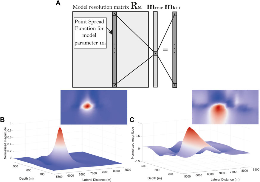
FIGURE 1. (A) The relationship between the true model ${\mathbf{m}}_{true}$ and the preferred inversion model ${\mathbf{m}}_{k+1}$ expressed as a matrix vector operation (1D case). (B) and (C) are examples of PSF for a well-resolved and poorly resolved 2D case, respectively. Both PSFs have been normalized to 1 for presentation purposes.

The concept of a PSF is well known from imaging theory (Rossmann, 1969) and describes how much a point or pixel in an image (i.e., a model parameter) is blurred due to the imaging system (a combination of acquisition system and choice of inversion algorithm in our case). A 2D image, as considered in this paper, is represented by a lexicographical ordering as illustrated in Figure 2. The resolution (blur) matrix then takes a more complex form as discussed in Section 3.2 (cf. Eq. 9). A perfectly resolved case exhibits a PSF with the value of 1 at the location of the image point and 0 elsewhere. Figures 1B, C show examples of a well-resolved and a poorly resolved case, respectively, for a 2D image. The PSF in Figure 1B is characterized by a small spread centered on the corresponding model parameter. However, in Figure 1C, the PSF is characterized by a large spread.

FIGURE 2

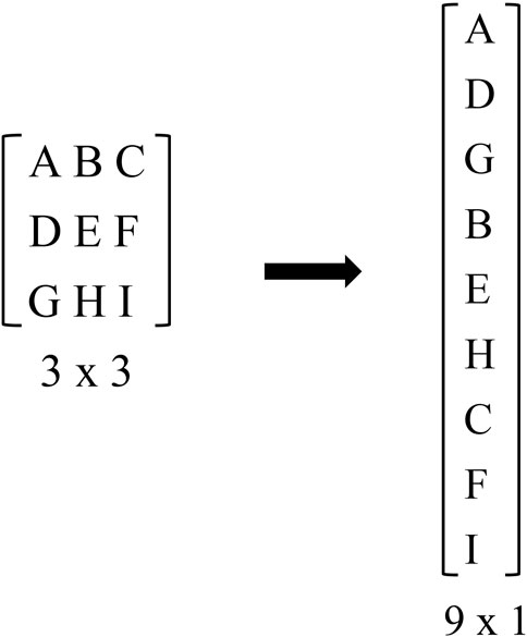
FIGURE 2. Lexicographical ordering of the 2D image (the letters indicate pixels).

3 General framework of deblurring

3.1 Forward (blur) model

From now on, we will use the notation A for the resolution matrix corresponding to a lexicographic ordering of the 2D image or model. The following general relationship between the true image $\mathbf{m}$ and its blurred counterpart $\mathbf{b}$ (i.e., the output from the CSEM inversion) holds (forward model)

$\mathbf{A}\mathbf{m}=\mathbf{b}+\mathbf{n},(8)$

where $\mathbf{A}$ is the blurring (resolution) matrix and $\mathbf{n}$ represents an additive noise term. Since $\mathbf{m}$ (and $\mathbf{b}$) is organized in lexicographical order (cf. Figure 2), the structure of the blur matrix takes a special form as discussed in the next section.

3.2 Blur matrix and a space-invariant PSF

We start by considering the case of a space-invariant PSF. Assume that the number of image points is M = 2N + 1 along each direction (and with indices running from -N to N). Assume also that the PSF has the same size as the image (cf. upper part of Figure 3). The first step in forming the blur matrix $\mathbf{A}$ is to organize each column of the PSF in a Toeplitz matrix as shown in the lower part of Figure 3 for row n.

FIGURE 3

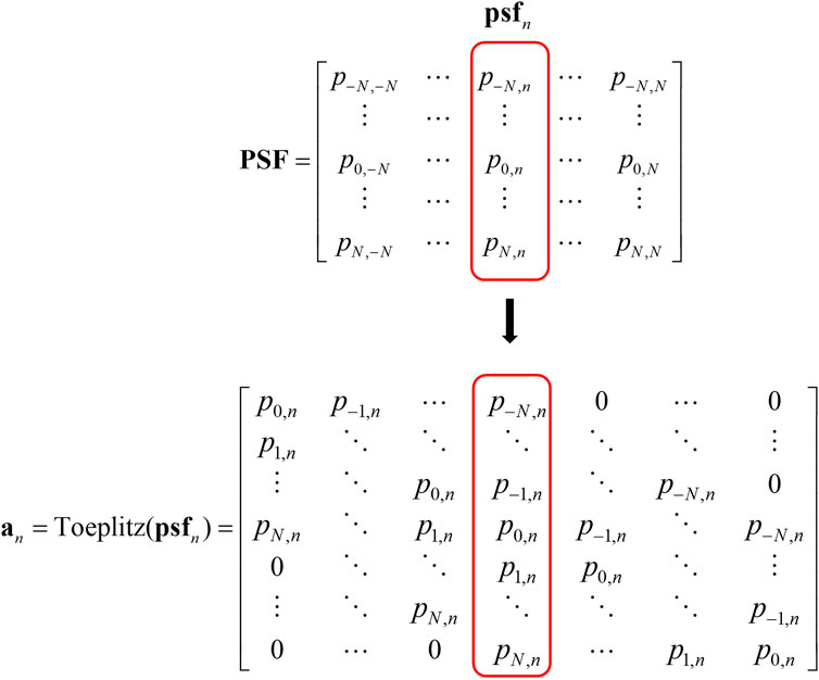
FIGURE 3. First step in forming the blur matrix $\mathbf{A}$: each column in the space-invariant PSF (upper part of the figure) is reorganized in a Toeplitz matrix as shown in the lower part of the figure.

The blur matrix $\mathbf{A}$ can now be constructed as a block Toeplitz matrix with Toeplitz blocks (BTTB) with zero boundary conditions (Hansen et al., 2006) and where each block element ${\mathbf{a}}_n\left(n=-N,.....-\mathrm{1,0,1}.....N\right)$ is defined in Figure 3:

$\mathrm{A}=\left[\begin{array}{ccccccc}{\mathbf{a}}_0& {\mathbf{a}}_{-1}& \cdots & {\mathbf{a}}_{-\mathrm{N}}& 0& \cdots & 0\\ {\mathbf{a}}_1& \ddots & \ddots & \ddots & \ddots & \ddots & ⋮\\ ⋮& \ddots & {\mathbf{a}}_0& {\mathbf{a}}_{-1}& \ddots & {\mathbf{a}}_{-\mathrm{N}}& 0\\ {\mathbf{a}}_{\mathrm{N}}& \ddots & {\mathbf{a}}_1& {\mathbf{a}}_0& {\mathbf{a}}_{-1}& \ddots & {\mathbf{a}}_{-\mathrm{N}}\\ 0& \ddots & \ddots & {\mathbf{a}}_1& {\mathbf{a}}_0& \ddots & ⋮\\ ⋮& \ddots & {\mathbf{a}}_{\mathrm{N}}& \ddots & \ddots & \ddots & {\mathbf{a}}_{-1}\\ 0& \cdots & 0& {\mathbf{a}}_{\mathrm{N}}& \cdots & {\mathbf{a}}_1& {\mathbf{a}}_0\end{array}\right].(9)$

The blur matrix A has dimensions $M^{2}x{M}^2 \mathrm{w}\mathrm{h}\mathrm{e}\mathrm{r}\mathrm{e} M=2N+1$.

3.3 Generalization to space-variant PSF (image segmentation)

To discuss a more general case characterized by space-variant PSFs, a pragmatic approach would be to subdivide the model space into space-invariant regions and perform deblurring separately for each region. This implies that each region is assigned a deblur matrix of the form given by Eq. 9, but with its own representative PSF. The final image is then constructed by combining the space-invariant regions after deblurring (and with possibly some smoothing applied to avoid edge effects). A more attractive approach, however, is to construct a space-variant A matrix (Nagy and O’Leary, 1997). Let Figure 4 represent an idealized case where the model space is horizontally split into two regions, each of them characterized by distinct and different PSFs. To minimize edge effects, a transition zone, which defines a gradual transition between the two PSFs, has also been introduced.

FIGURE 4

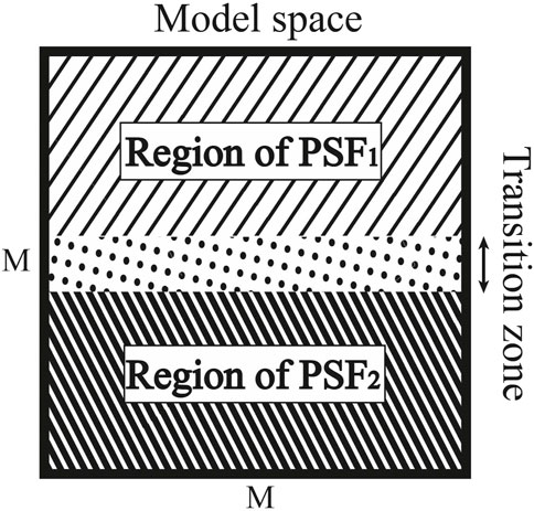
FIGURE 4. Idealized model space horizontally split into two regions including a transition zone. Note that this case has been chosen for illustration purposes of Eq. 10a (cf. Figure 5). In practical applications, both vertical and horizontal splitting can be employed (cf. Figure 8A).

Before constructing the space-variant blur matrix A, we need to define a corresponding space-invariant blur matrix for each subregion (same form as in Eq. 9). In the idealized case shown in Figure 4, two blur matrices (A₁ and A₂) need therefore to be constructed. In this demonstration example, we have defined the two PSFs as simple 2D Gaussian functions with different degrees of blurring. More specifically, we chose the PSF of region 1 to introduce less blurring than the corresponding PSF of region 2. This implies that the blur matrix A₁ has a more narrow band of values concentrated along its diagonal compared to the blur matrix A₂ (cf. upper row in Figure 5).

FIGURE 5

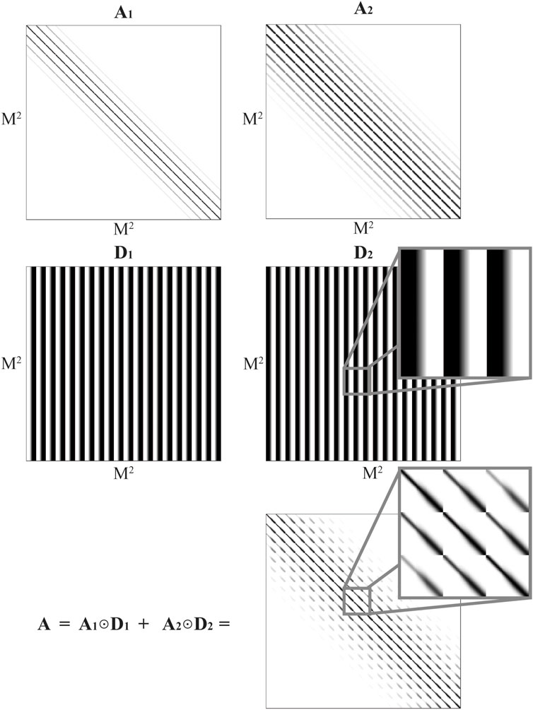
FIGURE 5. (Top row) Two space-invariant $\mathit{A}$-matrices corresponding to a well-resolved (${\mathit{A}}_{\mathbf{1}}$) and smeared (${\mathit{A}}_{\mathbf{2}}$) PSF. (Middle row) weighting matrices (${\mathit{D}}_{\mathbf{1}}\mathrm{a}\mathrm{n}\mathrm{d}{\mathit{D}}_{\mathbf{2}}$). (Bottom row) the space-variant $\mathit{A}$-matrix is calculated as the sum of the Hadamard product of the two space-invariant blur matrices and the associated weighting matrices.

The next step is to calculate a weighting matrix for each of the two regions in Figure 4 (D₁ and D₂). To avoid edge effects, the PSF should vary smoothly between different subregions. This can be achieved by applying linear tapering between neighboring subregions. In such a transition zone, an effective PSF is constructed as the linear combination between the two neighboring PSFs. The two weighting matrices for the idealized case in Figure 4 are shown in the middle row of Figure 5. A zoomed version of a section of the weight matrix D₂ is also included to better visualize the smooth transition between the two subregions (i.e., no sharp edges). The final blur matrix A can then be constructed as the sum of the Hadamard product of the two space-invariant matrices and the associated weighting matrices

$\mathbf{A}={\mathbf{A}}_1\odot {\mathbf{D}}_1+{\mathbf{A}}_2\odot {\mathbf{D}}_2,(\mathrm{10a})$

where the effective blur matrix A is shown in the bottom row of Figure 5. A zoomed version of a section of this matrix is also shown to better illustrate the effect of the smooth transition zone introduced between the two subregions in Figure 4.

For a general case with N regions, Eq. 10a generalizes to

$\mathbf{A}={\displaystyle \sum _{i=1}^N}{\mathbf{A}}_i\odot {\mathbf{D}}_i(\mathrm{10b})$

As the inversion can be sensitive to input parameters (e.g., the choice of PSFs and sizes of the transition zones), developing an interactive user interface to assist in the selection of the optimized parameters is crucial. Figure 6 shows the typical plot output from this user interface (i.e., the blurred model output from the CSEM inversion along with three selected PSFs). In an interactive system, a PSF plot (Figures 6B–D) automatically updates when clicking on the corresponding cell location in the blurred model (green dots in Figure 6A). This allows users to interactively evaluate whether a given PSF is suitable, and the user can then add this PSF to a list. After selecting the optimal PSFs, the user can define boundaries and the size of the transition zones (cf. Figure 5). This set of parametric choices is then used to construct the space-variant $\mathbf{A}$-matrix. This blur matrix A is stored in the memory of the user interface, allowing the user to efficiently test different sets of input parameters.

FIGURE 6

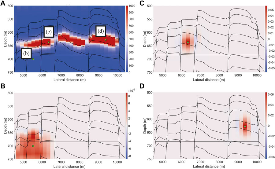
FIGURE 6. (A) Example of superimposed green dots in a blurred model, indicating the location of each of the PSFs shown in (B–D).

Nevertheless, the inversion is sensitive to the choice of PSFs. In the example shown in Figure 6, one of the PSFs corresponds to a poorly resolved model parameter (Figure 6B), whereas the PSFs in Figures 6C, D both describe a fairly well-resolved model parameter. These observations stress the important role our interactive user interface plays in controlling the quality of the selected parameters. The choice of an anomalous PSF (Figure 6B) can thus be easily avoided. In general, PSFs located (well) outside the target area should not be employed. Relevant PSFs are those near and inside the target area or structure. The PSFs in Figures 6C, D are examples of proper selections. It is well known that the output from a CSEM inversion is poorly resolved along the vertical direction. If the two PSFs in Figures 6C, D are used to construct the blur matrix, the corresponding deblurred image is expected to show improved vertical resolution. For a practical application, each PSF is delimited to a smaller area with tapering and normalization that ensures that the sum of its values inside the tapered area adds to 1.

3.4 Deblurring the CSEM inversion using NN-FCGLS

In this Section, we discuss how to deblur the output from the CSEM inversion. This step represents a new inversion problem to be solved, namely, the one with a forward model given by Eq. 8. Several solution alternatives exist, and in this study, we used the nonnegative flexible conjugate gradient least-squares (NN-FCGLS) algorithm (Gazzola et al., 2017), which is implemented as an inner-outer scheme. The updated model of the inner iteration can be written as

${\mathbf{m}}_{k+1}={\mathbf{m}}_k+{\alpha }_k{\mathbf{p}}_k,(11)$

where ${\alpha }_k$ is a bounded step size and ${\mathbf{p}}_k$ is a vector of direction. To fulfill the condition of nonnegativity in the solution space, the step size ${\alpha }_k$ is reduced so that ${\mathbf{m}}_{k+1}\ge 0 if{\mathbf{m}}_k>0$. In NN-FCGLS, this is accomplished using a bounded step size calculated with the following expression:

$\begin{array}{l}{\overline{\alpha }}_k={\alpha }_{k}if{\mathbf{p}}_k\ge 0\\ otherwise{\overline{\alpha }}_k=\min \left\{\begin{array}{l}{\alpha }_k,\min -{\left({\mathbf{m}}_k\right)}_j/{\left({\mathbf{p}}_k\right)}_j\\ j\in K\end{array}\right\},\end{array}(12)$

where K is a set of indices j such that ${\left({\mathbf{p}}_k\right)}_j<0$ and the direction ${\mathbf{p}}_k$ is obtained by a linear combination of at most ${\kappa }_k$ previously computed ${\mathbf{p}}_j$ with j varying in { max{0, k − ${\kappa }_k$},. . ., k−1}. If the maximum number of iterations k_max is assigned to the inner cycle, the choice ${\kappa }_k$ = k_max corresponds to a full recursion, while a lower ${\kappa }_k$ corresponds to a truncated recursion and with ${\kappa }_k$ = 1, only the last computed vector ${\mathbf{p}}_{k-1}$ is used. The outer cycle relies on suitable restarts to avoid stagnation. For further details about the algorithm, the reader is referred to Gazzola et al. (2017). In this study, we employed a code taken from the MATLAB library IR Tools (Gazzola et al., 2019).

Because the NN-FCGLS method enforces a nonnegativity constraint at each iteration, we consider that this algorithm will produce a more accurate approximate solution when the output from the CSEM inversion is a true nonnegative (i.e., log ($\rho$) and the resistivity $\rho$ is bounded by $\rho \ge$ 1 Ω-m) like in this case. The proposed deblurring approach is based on PSFs extracted from the resolution matrix associated with a linearized approximation of the original nonlinear problem. Thus, this procedure does not represent an exact solution to the blurring problem and the results obtained should always be treated with caution.

3.5 Blind deconvolution as a benchmark method

No precalculated PSFs are needed for blind deconvolution. This implies that the blur matrix $\mathbf{A}$ is now unknown, and the blind deconvolution technique estimates both the PSFs and the unknown “true” image $\mathbf{m}$ (Ayers and Dainty, 1988; Krishnamurthy et al., 1995; Holmes et al., 2006). To solve this joint problem in an efficient manner, the maximum likelihood estimation (MLE) principle is employed (van Trees, 1968). The main idea is to search for a statistical solution that maximizes the likelihood function, given some observations. Thus, the parameter values obtained (i.e., PSF and $\mathbf{m}$) are most likely to lead to the observed data. For more details, the reader is referred to Krishnamurthy et al. (1995) and Biggs and Andrews (1997).

In this paper, we applied blind deconvolution to benchmark our proposed approach, using the MATLAB routine deconvblind. It restores the image and the point-spread function (PSF) simultaneously employing the accelerated, damped Richardson-Lucy algorithm in each iteration (Richardson, 1972; Lucy, 1974).

4 Data demonstrations

4.1 Wisting oil field

The Wisting oil field is located in the southwestern Barents Sea. The reservoir is highly segmented and very shallow (approximately 250 m below the seafloor), and contains oil in sandstone from the late Triassic (Fruholmen Formation) and early Jurassic (Nordmela and Stø Formations) periods.

In this Chapter, we start by considering an idealized model of the Wisting field that can serve as a complex controlled-data case. Such a synthetic data set is vital to perform quality control in the proposed deblurring approach. The controlled-data example is then followed by a case where CSEM field data acquired across the Wisting field is employed.

4.2 Complex synthetic model

Figure 7 shows a plot of the synthetic model color-coded with vertical resistivity. Although the model includes anisotropy in most layers, we focus here on vertical resistivity because the CSEM method is known to be most sensitive to this polarization. For more details about the construction of the synthetic model, the reader is referred to Thorkildsen and Gelius (2023). Synthetic marine CSEM data were generated using the model shown in Figure 7, employing the MARE2DEM package in a forward-modeling mode. Five receivers evenly deployed on the seafloor at a 3000 m interval were used for the calculations. On the transmitter side, approximately 180 source positions were simulated using a spatial sample interval of around 200 m. Moreover, a total of 11 frequencies ranging from 0.2 to 12 Hz were included. Random noise with a standard deviation equal to 1% of the data amplitude was added to each recording.

FIGURE 7

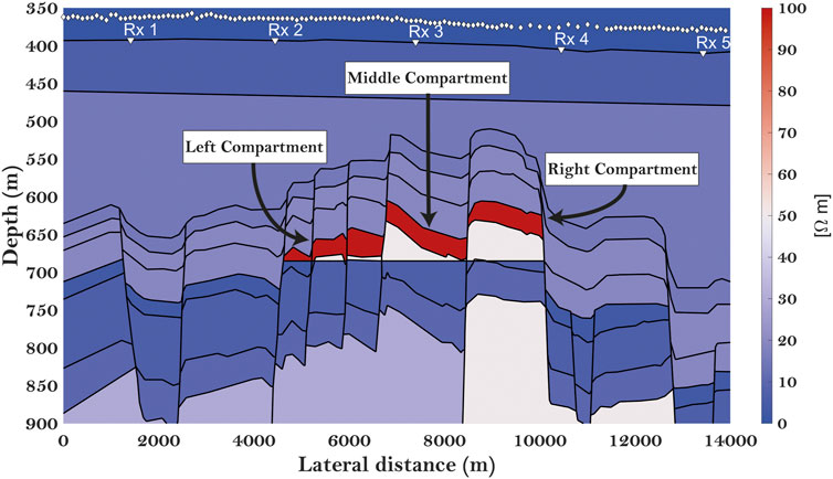
FIGURE 7. 2D synthetic model color-coded with vertical resistivity.

The blurred model obtained from the CSEM inversion is displayed in Figure 8A. The inversion was characterized by a smooth transition from the low resistivity background to the high resistivity inside the reservoir. During the inversion, we constrained the model update to a rectangular area enclosing the main reservoir, while keeping the rest of the model unchanged. We also employed a vertical sample interval of 5 m, which is denser than that normally employed in CSEM inversion. This was performed to enhance the deblurring effect from a visualization point of view. When compared to the “true” model in Figure 7, the inversion was able to reproduce the main features of the reservoir. However, the main resistive structure was too shallow for both the left and (parts of) the middle compartment. The white vertical lines introduced in Figure 8A indicate the borders between the different subregions employed when constructing the space-variant blur matrix A (transition zones not shown). In addition, ideal PSFs were introduced along the red frame surrounding the target region to constrain the outer parts of the image. An ideal PSF is a point-spread function that takes the value of 1 at the corresponding parameter location and 0 elsewhere.

FIGURE 8

FIGURE 8. (A) Blurred output from CSEM inversion of data generated in the complex synthetic model shown in Figure 7. The white vertical lines introduced indicate the borders between the different subregions employed when constructing the space-variant blur matrix. (B) Deblurred model obtained from NN-FCGLS after 12 iterations. (C) Output from blind deconvolution. Color scale between 0 and 250 Ω-m resistivity.

If we use the proposed deblurring approach, we generally expect to observe a better-resolved reservoir along the vertical direction (i.e., thinner). A direct comparison between the output from the CSEM inversion (Figure 8A) and the corresponding deblurred image obtained from NN-FCGLS (Figure 8B) supports this assumption. A total of six PSFs were employed during deconvolution (their actual locations are represented by the superimposed green dots in Figure 8). By using our interactive interface software the PSFs were carefully chosen based on visual inspection and extensive testing. After deblurring, the target structure appeared thinner overall and the right compartment showed the greatest change in resolution. This was also expected because that part of the reservoir is known to be the most poorly resolved. On the other hand, the result of blind deconvolution (Figure 8C) exhibited no resolution enhancement but rather the opposite. Note, however, that the blind deconvolution technique applied can only handle the case of a space-invariant (and unknown) PSF. The blind deconvolution result in Figure 8C was initialized employing a flat PSF. We also tested a Gaussian PSF as initialization but the results were poor. Use of multiple windows for both initializations did not improve the quality of the result.

4.3 CSEM field data

To demonstrate the effectiveness of the proposed method on field data, the proposed deblurring approach was applied to a 2D CSEM line extracted from the BSMC08W 3D survey acquired across the Wisting oil field during the summer of 2008 (with similar acquisition parameters as in the synthetic model case). We used data corresponding to a frequency range of 0.2–12 Hz (total of 23 frequencies) as the input for the CSEM inversion.

Figure 9A shows the blurred model obtained from an unconstrained CSEM inversion. This result was achieved after cubic interpolation of the originally coarser output grid resulting from MARE2DEM. This coarser inversion grid was sampled at 200 m laterally and 30 m vertically and was chosen in collaboration with the industry to ensure a reasonable computational time. However, the interpolated grid was sampled at 50 m laterally and 5 m vertically. Resampling of the image (and also selected PSFs) was performed to ensure that the deblurring step would be stable (otherwise, very few grid points would define both the blurred image and the corresponding PSFs). Figure 9A through C show superimposed arrows indicating an estimate of the average reservoir thickness (about 40 m).

FIGURE 9

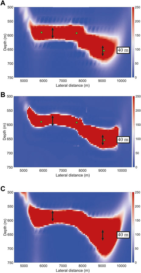
FIGURE 9. (A) Blurred output from the CSEM inversion of field data. (B) Deblurred model obtained from NN-FCGLS after six iterations. (C) Output from blind deconvolution. Color scale between 0 and 250 Ω-m resistivity.

Figure 9B displays the deblurred image obtained after six iterations of the NN-FCGLS method. A total of three carefully selected PSFs were employed during deconvolution (their actual locations are represented by the superimposed green dots in Figure 9). The overall effect of deconvolution is that the reservoir has become thinner and with sharper boundaries. In addition, the right portion of the reservoir, which was more poorly resolved, appears slightly uplifted. Due to the coarse sampling of the original inversion grid and the fact that Wisting is a thin reservoir, this field data example represents a limiting case. However, the vertical resolution of the deblurred image has still improved and is now closer to the known average reservoir thickness. Thus demonstrating the potential of the proposed method. By directly comparing the deblurred or deconvolved result (Figure 9B) with the result obtained through blind deconvolution (Figure 9C), it is clear that the latter technique does a poor job of deblurring. Employing blind deconvolution actually produces an image exhibiting lower resolution as compared to the original input.

5 Discussion and conclusion

Here, we investigated the feasibility of applying deblurring as a post-processing technique to enhance the resolution of the model output from a CSEM inversion. We developed a portfolio of supporting software for extracting the model resolution matrix associated with the CSEM inversion (MARE2DEM) and built the corresponding blur matrix, which can be used to correct the blurring described by the space-invariant PSFs. The actual deblurring was carried out using the nonnegative flexible gradient least-squares (NN-FCGLS) algorithm. Applications to both synthetic and field data demonstrated the potential of the proposed approach. In case of the synthetic data example, where the model is known, the deblurred CSEM image obtained employing our proposed approach matched the target layers well for all three compartments when compared with a superimposed structural mask of the Earth model. In case of the field data, the true Earth model is not exactly known, but the deblurred CSEM image using our proposed method seems to fit quite well with an expected average thickness of the reservoir of about 40 m (obtained from seismic interpretation).

Blind deconvolution was employed as a benchmark method and was shown to perform much poorer when applied to the same two data sets.

CSEM inversion is rather computationally intensive. For the data examples shown here, the inversion typically took several days to complete using a computer with 40 cpu’s and no memory constraints (within a 1% RMS error). Deblurring, on the other hand, is a very fast technique. The combined process of constructing the space-variant blur matrix A and running the actual deblurring was typically completed within minutes. Thus, repeated deblurring using different PSF choices is feasible.

Future work should address the optimal choice of PSFs for a given problem, and investigate further challenges associated with iterative convergence and the particular choice of inversion algorithm.

Data availability statement

The data analyzed in this study is subject to the following licenses/restrictions: proprietary data of EMGS ASA. Requests to access these datasets should be directed to https://emgs.com/about-us/contact-us/.

Author contributions

VT: methodology, construction of the Wisting synthetic model, inversion of CSEM synthetic and field data, calculation of the resolution matrix and PSFs, and manuscript writing. L-JG: concepts and methodology, manuscript writing, and revision. All authors contributed to the article and approved the submitted version.

Funding

This work was funded by the Research Centre for Arctic Petroleum Exploration (ARCEX) and the Norwegian Research Council (project number 228107).

Acknowledgments

The authors acknowledge EMGS ASA for providing the field data and Dr. Kerry Key for making the MARE2DEM package publicly available. The authors would also like to thank Silvia Gazzola, Per Christian Hansen, and James G. Nagy for making their software library IR Tools open access.

Conflict of interest

The authors declare that the research was conducted in the absence of any commercial or financial relationships that could be construed as a potential conflict of interest.

Publisher’s note

All claims expressed in this article are solely those of the authors and do not necessarily represent those of their affiliated organizations, or those of the publisher, the editors and the reviewers. Any product that may be evaluated in this article, or claim that may be made by its manufacturer, is not guaranteed or endorsed by the publisher.

References

Alumbaugh, D. L., and Newman, G. A. (2000). Image appraisal for 2-D and 3-D electromagnetic inversion. Geophysics 65 (5), 1455–1467. doi:10.1190/1.1444834

CrossRef Full Text | Google Scholar

Ayers, G. R., and Dainty, J. C. (1988). Iterative blind deconvolution method and its applications. Opt. Lett., 13 (7), 547–549. doi:10.1364/OL.13.000547

PubMed Abstract | CrossRef Full Text | Google Scholar

Biggs, D. S., and Andrews, M. (1997). Acceleration of iterative image restoration algorithms. Appl. Opt. 36 (8), 1766–1775.

PubMed Abstract | CrossRef Full Text | Google Scholar

Bjørke, A. K., Hansen, K. R., and Morten, J. P. (2020). Recovering stratigraphy orientation using TTI 3D CSEM Gauss-Newton inversion. SEG Technical Program Expanded Abstracts, 560–564. OnePetro, Richardson, TX, USA.

Google Scholar

Brown, V., Hoversten, M., Key, K., and Chen, J. (2012). Resolution of reservoir scale electrical anisotropy from marine CSEM data. Geophysics 77 (2), E147–E158.

CrossRef Full Text | Google Scholar

Chrapkiewicz, K., Wilde-Piórko, M., Polkowski, M., and Grad, M. (2020). Reliable workflow for inversion of seismic receiver function and surface wave dispersion data: A “13 BB star” case study. J. Seismol. 24 (1), 101–120.

CrossRef Full Text | Google Scholar

Constable, S. C., Parker, R. L., and Constable, C. G. (1987). Occam’s inversion: A practical algorithm for generating smooth models from electromagnetic sounding data. Geophysics 52 (3), 289–300.

CrossRef Full Text | Google Scholar

Constable, S. C. (2010). Ten years of marine CSEM for hydrocarbon exploration. Geophysics 75 (5), 75A67–75A81.

CrossRef Full Text | Google Scholar

Ellingsrud, S., Eidesmo, T., Johansen, S., Sinha, M. C., MacGregor, L. M., and Constable, S. (2002). Remote sensing of hydrocarbon layers by seabed logging (SBL): Results from a cruise offshore Angola. Lead. Edge 21 (10), 972–982.

CrossRef Full Text | Google Scholar

Fichtner, A., and Leeuwen, T. V. (2015). Resolution analysis by random probing. J. Geophys. Res. Solid Earth 120 (8), 5549–5573.

CrossRef Full Text | Google Scholar

Friedel, S. (2003). Resolution, stability and efficiency of resistivity tomography estimated from a generalized inverse approach. Geophys. J. Int. 153 (2), 305–316.

CrossRef Full Text | Google Scholar

Gazzola, S., Hansen, P. C., and Nagy, J. G. (2019). IR Tools: A MATLAB package of iterative regularization methods and large-scale test problems. Numer. Algor 81, 773–811.

CrossRef Full Text | Google Scholar

Gazzola, S., and Wiaux, Y. (2017). Fast nonnegative least squares through flexible Krylov subspaces. SIAM J. Sci. Comput. 39 (2), A655–A679.

CrossRef Full Text | Google Scholar

Grayver, A. V., Streich, R., and Ritter, O. (2014). 3D inversion and resolution analysis of land-based CSEM data from the Ketzin CO₂ storage formation. Geophysics 79 (2), E101–E114.

CrossRef Full Text | Google Scholar

Hansen, P. C., Nagy, J. G., and O’Leary, D. P. (2006). Deblurring images. Matrices, spectra and filtering. Society for Industrial and Applied Mathematics, Philadelphia, PA, USA.

Google Scholar

Holmes, T. J., Biggs, D., and Abu-Tarif, A. (2006). “Blind deconvolution,” in Handbook of biological confocal microscopy (Boston, MA, USA: Springer), 468–487.

CrossRef Full Text | Google Scholar

Hu, J., Schuster, G. T., and Valasek, P. A. (2001). Poststack migration deconvolution. Geophysics 66 (3), 939–952.

CrossRef Full Text | Google Scholar

Jackson, D. D. (1972). Interpretation of inaccurate, insufficient and inconsistent data. Geophys. J. Int. 28 (2), 97–109.

CrossRef Full Text | Google Scholar

Jakobsen, M., and Tveit, S. (2018). Distorted Born iterative T-matrix method for inversion of CSEM data in anisotropic media. Geophys. J. Int. 214, 1524–1537.

CrossRef Full Text | Google Scholar

Kalscheuer, T., Juanatey, M., Meqbel, N., and Pedersen, L. B. (2010). Non-linear model error and resolution properties from two-dimensional single and joint inversions of direct current resistivity and radiomagnetotelluric data. Geophys. J. Int. 182 (3), 1174–1188.

CrossRef Full Text | Google Scholar

Key, K. (2016). MARE2DEM: A 2-D inversion code for controlled-source electromagnetic and magnetotelluric data. Geophys. J. Int. 207 (1), 571–588.

CrossRef Full Text | Google Scholar

Krishnamurthy, V., Liu, Y. H., Bhattacharyya, S., Turner, J. N., and Holmes, T. J. (1995). Blind deconvolution of fluorescence micrographs by maximum-likelihood estimation. Appl. Opt. 34 (29), 6633–6647.

PubMed Abstract | Google Scholar

Lucy, L. B. (1974). An iterative technique for the rectification of observed distributions. Astronomical J. 79, 745–754.

CrossRef Full Text | Google Scholar

Mattsson, J. (2015). Resolution and precision of resistivity models from inversion of towed streamer EM data. SEG Technical Program Expanded Abstracts.

Google Scholar

Mckay, A., Mattson, J., and Du, Z. (2015). Towed streamer EM-reliable recovery of sub-surface resistivity. First Break 33 (4).

CrossRef Full Text | Google Scholar

Menke, W. (2012). Geophysical Data Analysis: Discrete Inverse Theory: MATLAB edition, 45. Academic Press, Cambridge, MA, USA.

Google Scholar

Nagy, J. G., and O'Leary, D. P. (1997). Fast iterative image restoration with a spatially varying PSF. Adv. Signal Process. Algorithms, Archit. Implementations VII. SPIE, 3162, 388–399.

CrossRef Full Text | Google Scholar

Nguyen, A. K., Nordskag, J. I., Wiik, T., Bjørke, A. K., Boman, L., Pedersen, O. M., et al. (2016). Comparing large-scale 3D Gauss-Newton and BFGS CSEM inversions. SEG Technical Program Expanded Abstracts, 872–877. OnePetro, Richardson, TX, USA.

CrossRef Full Text | Google Scholar

Ren, Z., and Kalscheuer, T. (2020). Uncertainty and resolution analysis of 2D and 3D inversion models computed from geophysical electromagnetic data. Surv. Geophys. 41 (1), 47–112.

CrossRef Full Text | Google Scholar

Richardson, W. H. (1972). Bayesian-based iterative method for image restoration. J. Opt. Soc. Am. 62, 55–59.

CrossRef Full Text | Google Scholar

Rossmann, K. (1969). Point spread-function, line spread-function, and modulation transfer function. Tools for the study of imaging systems. Radiology 93 (2), 257–272.

PubMed Abstract | CrossRef Full Text | Google Scholar

Routh, P. S., and Miller, C. R. (2006). “Image interpretation using appraisal analysis,” in Symposium on the application of geophysics to engineering and environmental problems (Society of Exploration Geophysicists), 1812–1820. Houston, TX, USA.

CrossRef Full Text | Google Scholar

Røsten, T., Johnstad, S. E., Ellingsrud, E., Amundsen, H. E. F., Johansen, S., and Brevik, I., A sea bed logging (SBL) calibration survey over the Ormen Lange gas field. Proceedings of the 65th EAGE Conference & Exhibition, P058, June 2003, Stavanger, Norway

Google Scholar

Sjoeberg, T. A., Gelius, L. J., and Lecomte, I. (2003). 2-D deconvolution of seismic image blur. Proceedings of the 2003 SEG Annual Meeting, Dallas, TX, USA, October 2003.

Google Scholar

Takahata, A. K., Gelius, L., Lopes, R., Tygel, M., and Lecomte, I. (2013). 2D spiking deconvolution approach to resolution enhancement of prestack depth migrated seismic images. Proceedings of the 75th EAGE Conference & Exhibition incorporating SPE EUROPEC 2013: June 2013, Netherlands.

CrossRef Full Text | Google Scholar

Thorkildsen, V. S., and Gelius, L.-J. (2023). Electromagnetic sensitivity: A CSEM study based on the Wisting oil field. Geophys. J. Int., 233, 3, 2124-2141. doi:10.1093/gji/ggad046

CrossRef Full Text | Google Scholar

Um, E. S., and Alumbaugh, D. L. (2007). On the physics of the marine controlled-source electromagnetic method. Geophysics 72 (2), WA13–WA26.

CrossRef Full Text | Google Scholar

Van Trees, H. L. (1968). Detection, estimation and modulation theory (Part I). New York, NY, USA: Wiley.

Google Scholar

Wang, F., Morten, J. P., and Spitzer, K. (2018). Anisotropic three-dimensional inversion of CSEM data using finite-element techniques on unstructured grids. Geophys. J. Int. 213 (2), 1056–1072.

CrossRef Full Text | Google Scholar

Xu, L., Sun, W-Q., Yan, Y-H., and Zhang, W-Q. (2020). Solar image deconvolution by generative adversarial network. Res. Astronomy Astrophysics 20 (11), 170–179.

CrossRef Full Text | Google Scholar

Yang, J., Huang, J., Zhu, H., McMechan, G., and Li, Z. (2022). An efficient and stable high-resolution seismic imaging method: Point-spread function deconvolution. J. Geophys. Res. Solid Earth 127, e2021JB023281.

CrossRef Full Text | Google Scholar

Yu, J., Hu, J., Schuster, G. T., and Estill, R. (2006). Prestack migration deconvolution. Geophysics 71 (2), S52–S63.

CrossRef Full Text | Google Scholar