Annual and semi-annual variations of electron density in the topside ionosphere observed by CSES

In this paper, based on the observations from Langmuir probe (LAP) onboard the China Seismo-Electromagnetic Satellite (CSES), the annual/semi-annual variations of electron density (Ne) measured at 02:00 and 14:00 local time (LT) in the topside ionosphere have been analyzed. Results indicated that the Ne exhibits an amplification-linear-saturation with the increase of P10.7 in the daytime, while roughly linear in the nighttime. The annual/semi-annual variations of CSES Ne at around 500 km are found by morphological analysis and Morlet wavelet analysis, with dominant period of 187 days and 374 days. The annual components of longitude-averaged Ne dominate at most magnetic latitudes (Mlats) with maxima around the June solstices in the northern hemisphere and the December solstice in the southern hemisphere (except for the northern hemisphere in the nighttime), while the semi-annual variation dominates at the magnetic equator and low magnetic latitudes with two maxima at equinoxes. The Ne dominant period is characterized by a transition from semi-annual variation at the equator and low magnetic latitudes regions to annual variation at the middle magnetic latitudes region. The annual/semi-annual variations of Ne observed by CSES satellite show a consistent performance with previous studies, and have complemented the ionospheric characteristics at 500 km altitude, especially in the nighttime.

1 Introduction

The Earth’s ionosphere is mainly produced via the photoionization of the upper atmosphere by energetic solar radiation and cosmic rays. It is an important part of the connection between near Earth environment and outer space, and has a significant impact on communications, broadcasting, navigation and positioning (Su et al., 1999; Su et al., 2010; Liu et al., 2011; Sardar et al., 2012). The ionosphere exhibits complex variations because of the influence from various factors such as the solar activity, geomagnetic activity, and local time (LT) etc. (Bilitza et al., 1990; Liu et al., 2009; Su et al., 2010; Slominska et al., 2013; Bhuyan et al., 2014; Su et al., 2016). Among them, the annual/semi-annual variations of ionospheric plasma density are one of the key scientific issues in ionospheric climatology, which have been widely studied in recent decades.

Early studies focused mainly on the annual/semi-annual variations characterization of peak electron density at the ionospheric F2 layer (NmF2), with the help of ground-based observation equipment. Yonezawa (1971) analyzed the seasonal, non-seasonal and semi-annual components of NmF2 from 9 pairs of stations at the middle and low latitudes. He found that at noon, non-seasonal component is generally the most important in the equatorial and low latitudes zone, while the semi-annual component always dominates at 15° magnetic latitude (Mlat). At the middle Mlat (±15° - ±40° Mlat), non-seasonal component is again the dominant one during low solar activity, but replaced by the semi-annual component as solar activity increases. At midnight, semi-annual component is the most important in the equatorial zone, and still dominate in low Mlat region for medium and higher solar activity. Ma et al. (2003) used ionospheric data (CD-ROM of Ionospheric Digital Database) observed from 30 stations located in 3 longitude sectors during 1974–1986 to analyze the semi-annual variation of NmF2. Their results indicated that the semi-annual variation of NmF2 appears almost at all geographic latitudes in the daytime (08:00–19:00 LT). For the nighttime (01:00–07:00 LT and 20:00–24:00 LT), NmF2 has semi-annual variation only in the region of geomagnetic equator within the two crests of ionospheric equatorial ionization anomaly (EIA). In the high latitude region, there is obvious semi-annual variation of NmF2 only in solar maxima years. As we can see, based on ground-based observations, annual/semi-annual variations of Ne have distinct latitudinal dependency both during daytime and nighttime. Liu et al. (2009) studied the seasonal variation of Ne profiles retrieved from the ionospheric radio occultation during daytime (13:00 LT) in the 200–560 km altitude range based on FORMOSAT-3/COSMIC (F3/C). They found at low altitudes a pronounced semi-annual component in the equatorial region and a strong annual variation in the near-pole region. At higher altitudes the semi-annual variation still predominates in equatorial region but gives way to annual variation in other regions. Such altitude dependence of Ne annual variation is consistent with observations from the middle and upper (MU) radar (Balan et al., 2000). Constellation Observing System for Meteorology, Ionosphere and Climate (COSMIC) data was analyzed to study the climatological variations of NmF2 in daytime (09:00–15:00 LT) during 2007–2010 (Burns et al., 2012). They found that at low latitudes (25° Mlat) the temporal variations are dominated by the semi-annual variation while annual variation dominated at high latitudes (75°Mlat). Using COSMIC occultation data during 2008–2011 in the daytime (12:00–14:00 LT), Ma (Ma et al., 2014) realized that annual and semi-annual variations of global NmF2 are strong in the middle and high latitudes, and weak in the low latitudes and equatorial region.

From these researches, annual/semi-annual variations of Ne are clear observed in the daytime; while only appear at a specific region or under certain solar activity levels in the nighttime. At the same time, more and more in situ observations were used to study annual/semi-annual variations in the topside ionosphere. Bailey et al. (2000) studied the annual variation of Ne at low latitudes (0–±25° Mlat) using the Hinotori satellite at 600 km altitude. They found that the semi-annual variation of Ne has maxima around the equinoxes and minima around the solstices both during daytime (09:00–17:00 LT) and nighttime (23:00–04:00 LT), which is also called semi-annual anomaly. Zhang and He (He et al., 2010; Zhang et al., 2014) studied the annual variation characteristics of Ne using the Detection of Electro-Magnetic Emissions Transmitted from Earthquake Regions (DEMETER) satellite data and found that Ne has strong annual variation during low solar activity at 660 km altitude, with semi-annual anomalies at middle and low latitudes both during daytime (10:30 LT) and nighttime (22:30 LT). The Ne annual/semi-annual variations are also examined by using data from the incoherent scatter radar (ISR) measurements. For example, Kawamura et al. (2002) studied the annual variation of the midlatitude ionosphere Ne observed at 200–600 km altitudes both during daytime (10:00–16:00 LT) and nighttime (22:00–05:00 LT) under low solar activity years, by using the MU radar (135° E, 35° N) observations. During the daytime, the annual variation with seasonal anomaly (larger Ne in winter compared to summer) is predominant at altitudes below the peak height of F2 layer (hmF2) while semi-annual variation is predominant at altitudes above hmF2. During the nighttime, the semi-annual variation disappear.

To sum up, the variations of Ne/NmF2 have been studied at 08:00–19:00 LT, 09:00–15:00 LT, 09:00–17:00 LT, 10:30 LT, 10:00–16:00 LT, 12:00–14:00 LT and 13:00 LT during the daytime and at 20:00–24:00 LT, 23:00–04:00 LT, 22:30 LT, 22:00–05:00 LT and 01:00–07:00 LT during the nighttime, respectively. It can be seen that the daytime ionosphere has been widely studied, especially in 10:00–14:00 LT, and the annual/semi-annual variations of Ne in the daytime are basically consistent in these studies. However, the nighttime ionosphere shows much more complex variations, and dedicated studies focused on the annual variation of nighttime ionosphere are pending. Besides, most of the studies are using the NmF2, while the in situ Ne observations at about 500 km altitude have not been well addressed.

With the launch of more and more satellites for ionospheric exploration, more abundant observations can be accumulated, providing opportunities to further study the ionosphere at different spatial and temporal scales under a variety of different conditions. The China Seismo-Electromagnetic Satellite (CSES), which is also called ZhangHeng-1 (ZH-1), was successfully launched on 2 February 2018. The satellite operates at ∼507 km, and the LT of descending and ascending nodes are 14:00 and 02:00 respectively. In this paper, we will study the annual/semi-annual variations of Ne with season and latitude under fixed orbit LT conditions based on CSES satellite observations, which complements the study of Ne at around 500 km. The second section is data description. The result is shown in the third section. Their characteristics and causes are discussed in Section 4, and Section 5 summarizes the results.

2 Data description

2.1 Data source

CSES is a sun-synchronous orbit satellite with an inclination of 97.4°, which aims to obtain global data of the electromagnetic field, plasma and energetic particles in the ionosphere and to study the ionospheric perturbations which could be possibly associated with seismic activity. Eight instruments are carried on the satellite, including Search-Coil Magnetometer (SCM), Electric Field Detector (EFD), High Precision Magnetometer (HPM), GNSS Occultation Receiver (GOR), Plasma Analyzer Package (PAP), Langmuir Probe (LAP), High Energetic Particle Package (HEPP) and Detector (HEPD), and Tri-Band Beacon (TBB) (Shen et al., 2018). In this paper, we mainly use the Ne data from the LAP. The operation modes of the LAP include survey mode and burst mode. The survey mode is used mainly to detect global Ne and electron temperature (Te), while the burst mode primarily allows detection of key areas, over China and within seismic belt (Liu et al., 2019). The CSES satellite have two fixed LT, 02:00LT and 14:00 LT, which can provide more detailed and comprehensive observations at the two identified local time sectors. Although there is a difference in absolute values of Ne observed by LAP onboard CSES with other ones (Yan et al., 2020; Pignalberi et al., 2022), the CSES Ne has been confirmed that there is a highly consistent relative variations with ones from the ISR at Millstone Hill, the Swarm satellite in similar orbital altitude, and the DEMETER satellite with a similar payload (Diego et al., 2019; Wang et al., 2019; Yan et al., 2020; Liu J. et al., 2021). In this paper we mainly focus on the periodic variations of Ne, which will not be affected by the absolute value of observation.

Data from May 2018 to April 2022 are used in this paper, in which the data from 22 June 2018 to 12 July 2018 aren’t available due to satellite commission test. It is worth pointing out that when one boom of EFD shades the LAP, there is a regular spike in the daytime Ne (Yan et al., 2022), and the spike interference has been removed in this study. In addition, in order to remove the effects of space weather activity and geomagnetic activity on the ionospheric variation, only the observations at Kp≤3 are selected.

2.2 Normalization of solar activity effects

Solar activity has important effects on the Ne of ionosphere (Liu et al., 2007a; Chen et al., 2008; Liu et al., 2011). We used the solar activity index P10.7 to check the solar activity effects, which is defined as $P10.7=\frac{\left(F10.7+F10.7A\right)}{2}$, where F10.7 is the solar 10.7-cm flux index, and F10.7A is the 81-day average of F10.7 centered on the day of interest (Lei et al., 2005; Bilitza et al., 2007; Liu L. B. et al., 2021). Figure 1 shows the time series of P10.7 and Ne in the range of ±10° Mlat during May 2018 and April 2022, with panel (A) and (B) representing the data in the daytime (14:00 LT) and nighttime (02:00 LT), respectively.

FIGURE 1

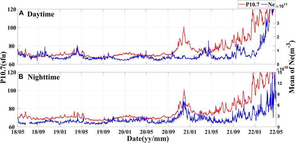
FIGURE 1. Time series of solar activity index P10.7 and Ne in the daytime(A), nighttime(B), the red line represents P10.7, and the blue line represents Ne.

From Figure 1, we found that the solar activity is quite low from May 2018 to September 2020, with P10.7 remaining around 70 sfu. After that it starts to gradually rise from the end of 2020, reaching 160 sfu in April 2022, which causes a significant increase in Ne. Therefore, in order to get more clear annual variation of Ne, P10.7 is used to normalize the Ne to reduce the influence of solar activity.

The distributions of daily mean Ne covering all Mlats and the corresponding P10.7 were represented in red scatter in Figure 2. The Ne in the daytime exhibits an amplification-linear-saturation effect with increasing of P10.7, which is consistent with previous researches (Chen et al., 2008; Chen et al., 2009; Bhuyan et al., 2014), while the relationship between Ne in the nighttime and P10.7 is roughly linear. Due to the distribution differences of Ne between daytime and nighttime, the P10.7 were divided into different bins, and the bin size of 5 sfu can ensure the fitted parameters of daytime data more exact, while 10 sfu size is enough for nighttime data. Then the mean value of P10.7 and Ne in each bin was calculated to study the correlation between them. The Ne in daytime was fitted to three segments according to mean value in each bin, and nighttime Ne to only one segment; where their fit lines are in black and error bars are marked with different colors. Finally, for the daytime, each Ne observation is normalized according to the fitting parameters of the y1 segment (Figure 2A) because most of Ne is in this segment, which represents the data effected by the vast majority of normal solar activity variation over 4 years. And considering that the Ne distribution of low P10.7 is abundant, a constant solar activity level at 100 sfu (P10.7) is chosen. That is, the formula $N{e}_{norm}=N{e}_{meas}\frac{a\cdot P+b}{a\cdot x+b}$ is used to normalize Ne, where P is a constant representing the normalized solar activity (P = 100), Ne_meas is the Ne measured by CSES, and a, b are the slope and intercept of the y1 fit (a = 0.4327, b = −11.95), respectively. The R marked in the bottom right corner stands for ’root mean square error’. For the nighttime, Ne was normalized to the y fit by the same method, among which P = 100, a = 0.8322, b = −47.99 (Figure 2B).

FIGURE 2

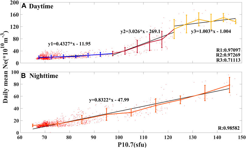
FIGURE 2. The distribution of Ne with P10.7 at daytime (A) and nighttime (B).

Therefore, the Ne used in this paper is not the actual observations, but the Ne values normalized according to the fitting relationship between Ne and P10.7 in the daytime and nighttime, respectively.

3 Results

3.1 Global distribution of Ne

The annual variation of Ne on the global scale was investigated by constructing global distribution maps. The map was divided into cells with ΔLat = 2.5° and ΔLong = 5°. The mean value of Ne in each cell was calculated using all the available data as a function of the position over a given time. To represent the global characteristics of Ne more clearly, the logarithm of Ne is used, and the global distribution of log10(Ne) in the daytime and nighttime are shown in Figures 3, 4. A uniform range of Ne value is used to better compare variation. From top to bottom are the results of the same season in different years, and from left to right the different seasons: Jun. solstice (May-August), Sep. equinox (September-October), Dec. solstice (November and December to January and February of the following year), and Mar. equinox (March-April). The black solid line marks the magnetic equator.

FIGURE 3

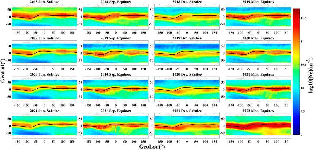
FIGURE 3. Global distribution of Ne in the daytime. From top to bottom represent different years of the same season, and from left to right correspond to different seasons: Jun. solstice (May-August), Sep. equinox (September-October), Dec. solstice (November to February of the following year), and Mar. equinox (March-April). The black solid line marks the magnetic equator. Ne is colored according to the colorbar on the right. The month information for each subplot is marked at the top.

FIGURE 4

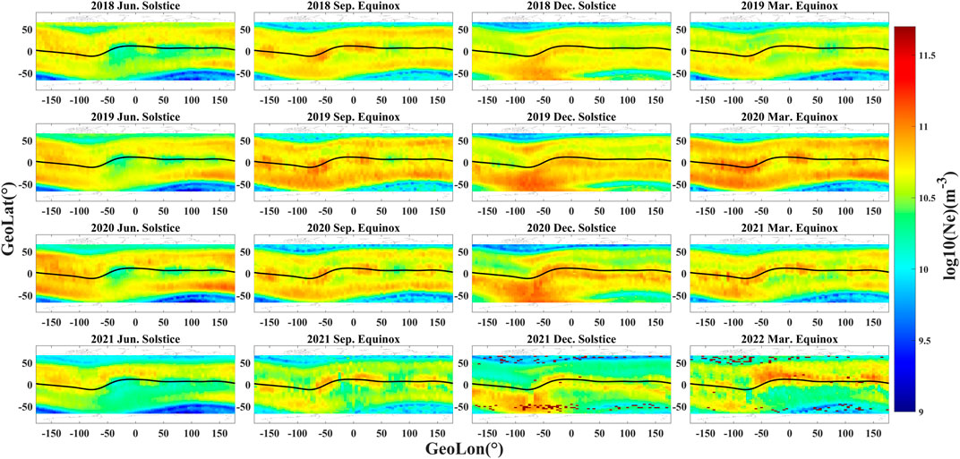
FIGURE 4. Same as Figure 3 but for Ne during nighttime.

It can be seen that the EIA structure is pronounced and varies significantly with the seasons (Figure 3). The high Ne area at the equinoxes is symmetrical about the magnetic equator. For solstice seasons, the high Ne value at the summer (winter) solstice is located in the geomagnetic northern (southern) hemisphere, showing the asymmetric characteristics of the northern and southern hemispheres. The intensity of Ne at the equinoxes is the strongest (stronger in the Mar. equinox than that in the Sep. equinox), and weaker in Jun. solstice and weakest in Dec. solstice.

The global distribution of nighttime Ne (Figure 4) differs from that of the daytime (Figure 3). The nighttime Ne has significant characteristics for each season, a distinct 3/4-wave structure are exhibited at two equinoxes and symmetric about the magnetic equator; the Weddell Sea Anomaly (WSA, Ryu et al., 2016) phenomenon in the southern hemisphere is obvious in the Dec. solstice.

From Figures 3, 4, the global distribution map of Ne in both the daytime and nighttime has obvious annual and seasonal variation; there is an asymmetry between the northern and southern hemispheres almost at all solstices.

3.2 Annual/semi-annual variations characteristics at different Mlats

In order to further check the annual variation feature of Ne, its detailed information is analyzed at different Mlat regions. The daily longitude-averaged values of Ne are computed at different Mlats and shown in Figures 5, 6. The annual trends of Ne from 55° N to 55° S Mlat are shown with the Mlat interval separated by 5°, including daytime and nighttime data during four consecutive years from May 2018 to April 2022. The red line and blue line represent data in the northern hemisphere (NH) and the southern hemisphere (SH), respectively. For example, the Ne at 0° Mlat is represented by the average of all longitudes observed within 2.5° N to 2.5° S Mlat.

FIGURE 5

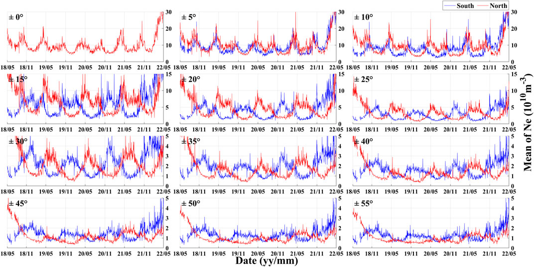
FIGURE 5. Temporal variation of daytime Ne in different Mlats ranges. Results are presented from the equator to ±55° Mlat with 5° intervals. Each subplot represents the daily mean Ne variation at different Mlats range. The blue line represents data in the southern hemisphere and the red line represents data in the northern hemisphere.

FIGURE 6

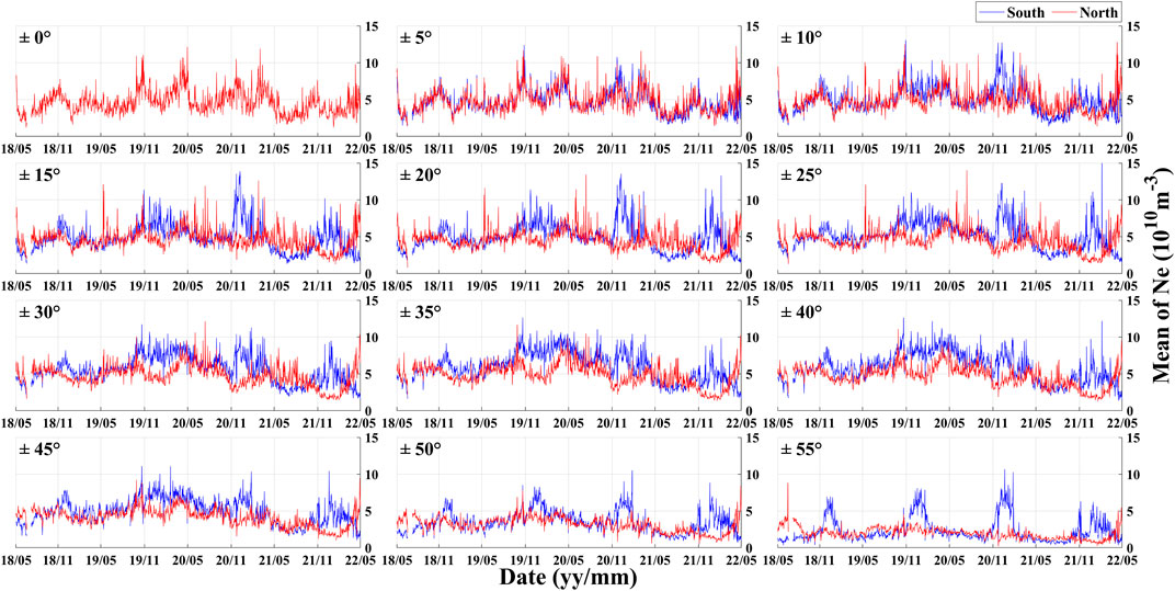
FIGURE 6. Same as Figure 5 but for Ne during nighttime.

From Figure 5, within the range of ±10° Mlat, semi-annual variation of Ne for the daytime is quite prominent. There are maximum at around equinoxes and minimum at around solstices, with consistent variation in both the NH and SH, which is also called semi-annual anomaly. With the increasing of Mlats, the stable semi-annual variation gradually changed to annual variation within ±15° to ±25° Mlat, and the consistent annual variation of Ne in both the NH and SH gradually turned into the opposite, but with the same value range. A stable annual variation of Ne at around ±30° to ±40° Mlat are shown, and the trend of annual variation in the NH and SH is exactly opposite, with maximum at Dec. solstice and minimum at the Jun. solstice in the SH, and the opposite in NH. The annual variation of Ne starts to weaken since ±45° Mlat. It should be noted that the value of Ne is drastically decreasing with increasing Mlats, so the ordinates take different values range to express the annual variation clearly at different Mlats.

The Ne variation in the nighttime is shown in Figure 6, where data in both NH and SH exhibit semi-annual variation near the equator just the same as daytime. With the increasing of Mlats, the semi-annual variation in NH and SH begin to differ. In the SH, the semi-annual variation changes into annual variation near 10° S Mlat, forming a stable annual variation characteristic at 15° S to 25° S Mlat, with maximum at Dec. solstice and minimal at Jun. solstice. The annual variation characteristics become irregular with increasing latitude in 30° S to 45° S Mlat, and a stable annual variation characteristic is formed again in 50° S to 55° S Mlat. Data in the NH shows semi-annual variation at 0°–15° N Mlat, then a clear annual variation feature is found in the range of 20° N to 35° N Mlat; while the annual variation feature is not obvious from 40° N Mlat and then disappear at 45° N to 55° N Mlat.

To sum up, both daytime and nighttime Ne have annual and semi-annual variations, and the annual/semi-annual variations of Ne in the daytime are clearer and more defined than ones in the nighttime. The peak and valley characteristics are different at different Mlats in the NH and SH.

3.3 The period of annual/semi-annual variations

To further check the periodic information of Ne at different Mlats, Morlet wavelet analysis is carried out on the time series of Ne data, such as the Ne data at ±5° Mlat, as shown in Figure 7, where the left columns are the Wavelet Power Spectrum results, and the right columns represent results of the Global Wavelet Spectrum (GWS), the dashed red lines are the 95% confidence levels in GWS. The (A), (B), (C), (D) correspond to the results of daytime Ne in SH and NH, as well as nighttime Ne in SH and NH. Taking Figure 7A as an example, the Y-axes are the periods of Ne, the X-axis in left column represent the time-span ranging from May 2018 to April 2022, and X-axis in right column correspond to Power. Results show that the dominant period are mainly at about 187 days and 374 days, representing the semi-annual and annual variations of the ionosphere Ne, with the semi-annual period being slightly stronger than the annual period. Apparently the annual/semi-annual period results for ±5° Mlats all pass the 95% significance level.

FIGURE 7

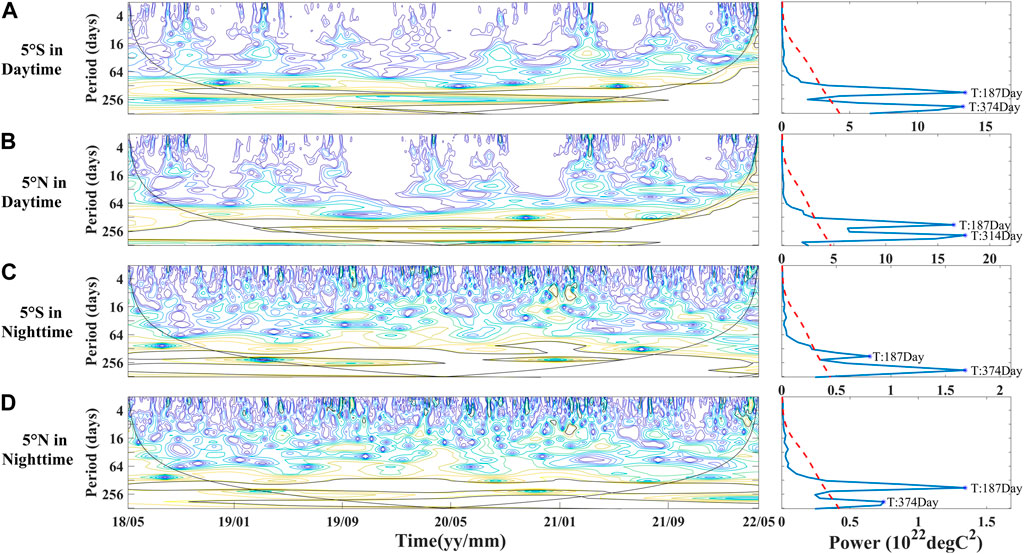
FIGURE 7. The Spectral analysis results using Morlet wavelet analysis for Ne during ±5° Mlat at daytime SH(A), NH(B) and at nighttime in SH(C), NH(D), respectively. The left columns show the Wavelet Power Spectrum results, while the right columns show the results of Global Wavelet Spectrum (GWS), and the dashed red lines are the 95% confidence levels.

The results of all the time series in Figures 5, 6 have been calculated by Morlet wavelet analysis, and their most dominant period of Ne are displayed in Table 1, which from top to bottom are daytime data in the NH and SH, as well as nighttime data in the NH and SH separately. Results in Table 1 are all above the 95% confidence level. Ne in both the daytime and nighttime have distinct annual/semi-annual periods at all Mlats. One of the common periods is 187 days, which is very close to the semi-annual period of 187.7 days observed by Guo et al. (2015) in the Global Total Electron Content (TEC) measurements. The Ne dominant period is characterized by a transition from semi-annual variation at the equator and low Mlat to annual variation at middle Mlat. From Table 1, we find that the transition concentrated in the range of ±5° - ±15° Mlat in both the daytime and nighttime.

TABLE 1

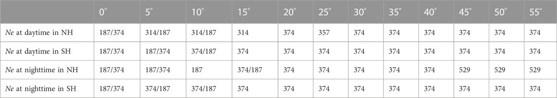
TABLE 1. Chromatography conditions.

4 Discussions

In this paper, the annual/semi-annual periods are clearly observed: the semi-annual periods are mostly dominant in the equatorial and low Mlats (0°–±5° Mlat) and the annual variation periods dominated in the middle Mlat (±15°–±55° Mlat), which is clearer in the daytime than nighttime. Although a similar period of Ne in the nighttime is found, the morphology of variation is significantly different from that in the daytime.

The period of daytime Ne is simple and clear. The EIA is the main structure at equatorial and low Mlats in all seasons with the semi-annual variation near the equator (Figure 3), and the transition between ±5°–±15° Mlat and the annual variation at middle Mlat are clear in both the NH and SH (Figure 5), which is consistent with the previous researches (Burns et al., 2012). However, the period of nighttime Ne is complicated. There is a consistent semi-annual variation near the equator, while for the mid-latitude region, the annual/semi-annual variations are less apparent in terms of the time series morphology of the NH, which is inferred to be related to some abnormal structure, such as the midlatitude summer nighttime anomaly (MSNA, Thampi et al., 2011), and the midlatitude ionospheric trough (MIT, Matyjasiak et al., 2016). These structures don’t appear in annual/semi-annual period, but in more random ones, thus smoothing the trend of annual/semi-annual variations. For the SH, the annual variation characteristics of Ne are more influenced by the WSA (mainly concentrated in the Dec. solstice, as shown in Figure 4). These seasonal characteristic structures in the nighttime have a direct impact on the Ne, so that there is a more pronounced annual/semi-annual variations of Ne in the SH compared to the NH. In addition, although the morphology of annual/semi-annual variations is not obvious, the Morlet wavelet analysis results confirmed that the most dominant periods of Ne remain 187 days and 374 days (Table 1) at all Mlats.

Using International GNSS Service (IGS) data, annual/semi-annual variations of TEC were studied by Yu et al. (2006), and results showed that the magnitude of the annual variation of TEC during daytime (14:00 LT) is larger at mid and high latitudes than equatorial and low latitudes. And the magnitude of the semi-annual variation of TEC is larger at equatorial region and slightly smaller at mid-latitudes. Shi et al. (2015) concluded that the semi-annual variation is obvious outside the near-polar region in the NH and the south American region in the SH during daytime (08:00–19:00 LT), and the semi-annual variation is only obvious at low latitudes during nighttime (19:00–8:00 LT). Natali et al. (2011) studied vertical TEC data derived from global GPS and found that at noon it is possible to see patterns of the seasonal variation, semi-annual anomaly, while at night there is no evidence of seasonal or annual anomaly for any region, but it is possible to see the semi-annual anomaly at low latitudes with a sudden decrease towards midlatitudes; Yu et al. (2004b) used NmF2 data in the daytime (14:00 LT) during six high solar activity years and found the annual variation are most pronounced at ±40°–±60° Mlat. The semi-annual variation is generally weak in the near-pole region and strong in the far-pole region of both hemispheres. Using data from DEMETER and Defense Meteorological Satellite Program (DMSP), annual variation of Ne and total ion density (Ni) are studied by Zhang et al. (2014); He et al. (2010); Liu et al. (2007b). They found that the Ne has strong annual variation, with semi-annual anomalies at middle and low latitudes in both daytime (10:30 LT) and nighttime (22:30 LT), while annual components of longitude-averaged Ni dominate at most latitudes in the daytime (09:30 LT) and nighttime (21:30 LT). Balan et al. (2000) used MU radar data found that at nighttime (22:00–05:00 LT) the annual variation component dominates at all heights, while the seasonal anomaly and semi-annual variation disappear.

From above researches using the data of TEC, NmF2 and in situ Ne, Ni, the annual/semi-annual variations of Ne in daytime are clearly evidenced. For nighttime, although some studies have found annual/semi-annual variations, some researches revealed that the annual and semi-annual variation of Ne are absent at midlatitudes in both hemispheres. In this paper, both morphological analysis and Morlet wavelet analysis were used to confirm that the semi-annual periods are mostly dominant in the equatorial and low Mlat (0°–±5° Mlat) and the annual variation periods are mostly dominant in the middle Mlat (±15°–±55° Mlat). These results in this study partially confirm the conclusions of previous studies.

The ionospheric photochemical generation rate, indicators of geomagnetic, tide, content of neutral components and thermospheric circulation and composition are the main reasons of annual/semi-annual variations (Zou et al., 2000; Yu et al., 2004b; Scott et al., 2015; Shi et al., 2015; Ghimire et al., 2022). Qian et al. (2013) found that variable eddy diffusion may play an important role in the observed variation of NmF2 at low latitudes and changes in turbulent mixing drives the annual/semi-annual variations in both the neutral and ionized components of the coupled system. Yu et al. (2004a) gave a clear semi-annual variation pattern of the ionospheric electric field in the middle and low latitudes and equatorial regions. At low and middle latitudes, the electric field has a strong control on the structure and motion of the ionospheric plasma, so the semi-annual variation of the electric field should have a significant effect on the observed semi-annual variation of the ionospheric NmF2 at low and middle latitudes and at equatorial regions. The ionosphere is mainly generated through photoionization of the upper atmosphere by solar EUV and X-ray radiation. It is strongly influenced by photoionization during daytime. While the photoionization process in the F region during nighttime is negligible, and is controlled by both the recombination processes and the ionospheric dynamics (Chen et al., 2008; Le et al., 2017). Therefore, for the daytime, the variation of Ne has a very direct relationship with the sunlight illumination, so it shows seasonal and annual periodicity changes consistent with the variation of the solar illumination, and the variation of Ne in different latitudes varies with the location from the Sun. At nighttime, although the changes of sunlight are also affected, recombination processes and the ionospheric dynamics play a more important role, coupled with the appearance of different night anomalous structures, so the changes of Ne are more complex, and thus annual/semi-annual variations intensity is weaker.

There are two other phenomena worth to be noted. Firstly, as can be seen in Figure 6, Ne is significantly lower in the range of 45° N to 60° N Mlat in the nighttime than in the other latitudinal ranges. According to the research (Yan et al., 2022), there is a sudden drop in Ne from mid-March to mid-September each year when the satellite flies out from shadow into the sunlight side with a yearly growth of its amplitude. And the position of the shadow varying at geo-latitudes from 40° N to 65° N, which coincides with the lowering of Ne as we can see in Figure 6 (shown by the red line in the fourth row). Secondly, a 529 days period occurs above 45° N Mlat in the nighttime, which may be related to more complex regions of the NH such as MSNA and MIT.

5 Conclusion

Using in situ Ne data observed by the LAP onboard CSES satellite from May 2018 to April 2022, we studied the annual/semi-annual variations of Ne both at 14:00 LT and 02:00 LT. The results are summarized as follows:

1. Daily mean Ne exhibits an amplification-linear-saturation effect with the increasing of P10.7 in the daytime, while a linear increase is observed at nighttime.

2. It is clear that Ne at around 500 km exhibits annual/semi-annual variations in both the daytime and nighttime, which is much clearer in daytime.

3. The annual/semi-annual variations of Ne in the daytime show latitudinal dependence, with opposite annual variation characteristics between the northern and southern hemispheres.

4. Although the annual variation of Ne in the nighttime is not particularly pronounced like ones of the daytime, especially in the northern hemisphere, the stable annual/semi-annual variations of Ne in the nighttime are still observed both from morphological analysis and from Morlet wavelet analysis.

5. The Ne dominant period is characterized by a transition from semi-annual variation at the equator and low Mlat to annual variation at middle Mlat. The transition region concentrated in the range of ±5° to ±15° Mlat in both daytime and nighttime.

Data availability statement

The original contributions presented in the study are included in the article/supplementary material, further inquiries can be directed to the corresponding author.

Author contributions

KZ, RY, and CX contributed to conception and design of the study. KZ and RY wrote the first draft of the manuscript. CX, ZZ, XS, YG, and CL provided guidance and comments on the paper. DL, SX, FG, and NZ organized the database. LZ and FL were mainly responsible for the experimental part. All authors contributed to manuscript revision and approved the submitted version.

Funding

This work was supported by the Fundamental Research Funds for NINH (Grant No. ZDJ2019-22), National Key R & D Program of China (Grant No. 2018YFC1503502-06), the Dragon five cooperation (Grant No. 59236), the APSCO earthquake Project Phase II, the Stable-Support Scientific Project of CRIRP (Grant No. A132001W07) and ISSI-BJ.

Acknowledgments

Thanks to the Kp index download from site https://wdc.kugi.kyoto-u.ac.jp/wdc/Sec3.html and F10.7 index download from the site https://www.spaceweather.gc.ca/forecast-prevision/solar-solaire/solarflux/sx-5-flux-en.php. The authors acknowledge CSES mission (http://www.leos.ac.cn) for providing the electron density data, which is funded by China National Space Administration (CNSA) and China Earthquake Administration (CEA).

Conflict of interest

The authors declare that the research was conducted in the absence of any commercial or financial relationships that could be construed as a potential conflict of interest.

Publisher’s note

All claims expressed in this article are solely those of the authors and do not necessarily represent those of their affiliated organizations, or those of the publisher, the editors and the reviewers. Any product that may be evaluated in this article, or claim that may be made by its manufacturer, is not guaranteed or endorsed by the publisher.

References

Bailey, G. J., Su, Y. Z., and Oyama, K. I. (2000). Yearly variations in the low-latitude topside ionosphere. Ann. Geophysicae-Atmospheres Hydrospheres Space Sci. 18 (7), 789–798. doi:10.1007/s00585-000-0789-0

CrossRef Full Text | Google Scholar

Balan, N., Otsuka, Y., Fukao, S., Abdu, M. A., and Bailey, G. J. (2000). “Annual variations of the ionosphere: A review based on MU radar observations,” in Lower ionosphere: Measurements and models. Editors K. M. Rawer, D. K. Bilitza, K. I. Oyama, and W. Singer, 25, 153–162. doi:10.1016/s0273-1177(99)00913-8

CrossRef Full Text | Google Scholar

Bhuyan, P. K., and Bora, S. (2014). Solar cycle effect on temporal and spatial variation of topside ion density measured by SROSS C2 and ROCSAT 1 over the Indian longitude sector. Adv. Space Res. 54 (3), 290–305. doi:10.1016/j.asr.2013.07.017

CrossRef Full Text | Google Scholar

Bilitza, D., Truhlik, V., Richards, P., Abe, T., and Triskova, L. (2007). Solar cycle variations of mid-latitude electron density and temperature: Satellite measurements and model calculations. Adv. Space Res. 39 (5), 779–789. doi:10.1016/j.asr.2006.11.022

CrossRef Full Text | Google Scholar

Bilitza, D., and Hoegy, W. (1990). Solar activity variation of ionospheric plasma temperatures. Adv. Space Res. 10 (8), 81–90. doi:10.1016/0273-1177(90)90190-b

CrossRef Full Text | Google Scholar

Burns, A. G., Solomon, S. C., Wang, W., Qian, L., Zhang, Y., and Paxton, L. J. (2012). Daytime climatology of ionospheric N_mF₂ and h_mF₂ from COSMIC data. J. Geophys. Res. Space Phys. 117 (A9). doi:10.1029/2012ja017529

CrossRef Full Text | Google Scholar

Chen, Y. D., Liu, L. B., and Le, H. J. (2008). Solar activity variations of nighttime ionospheric peak electron density. J. Geophys. Research-Space Phys. 113 (A11), A11306. doi:10.1029/2008ja013114Article

CrossRef Full Text | Google Scholar

Chen, Y. D., Liu, L. B., Wan, W. X., Yue, X. N., and Su, S. Y. (2009). Solar activity dependence of the topside ionosphere at low latitudes. J. Geophys. Research-Space Phys. 114, A08306. doi:10.1029/2008ja013957Article

CrossRef Full Text | Google Scholar

Diego, P., Coco, I., Bertello, I., Candidi, M., and Ubertini, P. (2019). Ionospheric plasma density measurements by Swarm Langmuir probes: Limitations and possible corrections. Ann. Geophys. Discuss., 1–15. doi:10.5194/angeo-2019-136

CrossRef Full Text | Google Scholar

Ghimire, B. D., Gautam, B., Chapagain, N. P., and Bhatta, K. (2022). Annual and semi-annual variations of TEC over Nepal during the period of 2007-2017 and possible drivers. Acta Geophys. 70 (2), 929–942. doi:10.1007/s11600-021-00721-3

CrossRef Full Text | Google Scholar

Guo, J., Li, W., Liu, X., Kong, Q., Zhao, C., and Guo, B. (2015). Temporal-spatial variation of global GPS-derived total electron content, 1999-2013. PLoS One 10 (7), e0133378. doi:10.1371/journal.pone.0133378

PubMed Abstract | CrossRef Full Text | Google Scholar

He, Y. F., Yang, D. M., Zhu, R., Qian, J. D., and Parrot, M. (2010). Variations of electron density and temperature in ionosphere based on the DEMETER ISL data. Earthq. Sci. 23 (4), 349–355. doi:10.1007/s11589-010-0732-8

CrossRef Full Text | Google Scholar

Kawamura, S., Balan, N., Otsuka, Y., and Fukao, S. (2002). Annual and semiannual variations of the midlatitude ionosphere under low solar activity. J. Geophys. Research-Space Phys. 107 (A8), SIA 8-1–SIA 8-10. doi:10.1029/2001ja000267Article 1166

CrossRef Full Text | Google Scholar

Le, H. J., Yang, N., Liu, L. B., Chen, Y. D., and Zhang, H. (2017). The latitudinal structure of nighttime ionospheric TEC and its empirical orthogonal functions model over North American sector. J. Geophys. Research-Space Phys. 122 (1), 963–977. doi:10.1002/2016ja023361

CrossRef Full Text | Google Scholar

Lei, J. H., Liu, L. B., Wan, W. X., and Zhang, S. R. (2005). Variations of electron density based on long-term incoherent scatter radar and ionosonde measurements over Millstone Hill. Radio Sci. 40 (2), Rs2008. doi:10.1029/2004rs003106Article

CrossRef Full Text | Google Scholar

Liu, C., Guan, Y. B., Zheng, X. Z., Zhang, A. B., Piero, D., and Sun, Y. Q. (2019). The technology of space plasma in-situ measurement on the China Seismo-Electromagnetic Satellite. Sci. China-Technological Sci. 62 (5), 829–838. doi:10.1007/s11431-018-9345-8

CrossRef Full Text | Google Scholar

Liu, J., Guan, Y. B., Zhang, X. M., and Shen, X. H. (2021a). The data comparison of electron density between CSES and DEMETER satellite, Swarm constellation and IRI model. Earth Space Sci. 8 (2), e2020EA001475. doi:10.1029/2020ea001475Article

CrossRef Full Text | Google Scholar

Liu, L. B., Chen, Y. D., and Le, H. J. (2021b). Response of the ionosphere to varying solar fluxes. Up. Atmos. Dyn. Energetics, 301–324. doi:10.1002/9781119815631.ch16

CrossRef Full Text | Google Scholar

Liu, L. B., Wan, W. X., Chen, Y. D., and Le, H. J. (2011). Solar activity effects of the ionosphere: A brief review. Chin. Sci. Bull. 56 (12), 1202–1211. doi:10.1007/s11434-010-4226-9

CrossRef Full Text | Google Scholar

Liu, L. B., Zhao, B. Q., Wan, W. X., Ning, B. Q., Zhang, M. L., and He, M. S. (2009). Seasonal variations of the ionospheric electron densities retrieved from Constellation Observing System for Meteorology, Ionosphere, and Climate mission radio occultation measurements. J. Geophys. Research-Space Phys. 114, A02302. doi:10.1029/2008ja013819Article

CrossRef Full Text | Google Scholar

Liu, L., Wan, W., Yue, X., Zhao, B., Ning, B., and Zhang, M. L. (2007a). The dependence of plasma density in the topside ionosphere on the solar activity level. Ann. Geophys. 25 (6), 1337–1343. doi:10.5194/angeo-25-1337-2007

CrossRef Full Text | Google Scholar

Liu, L., Zhao, B., Wan, W., Venkartraman, S., Zhang, M. L., and Yue, X. (2007b). Yearly variations of global plasma densities in the topside ionosphere at middle and low latitudes. J. Geophys. Research-Space Phys. 112 (A7), A07303. doi:10.1029/2007ja012283Article

CrossRef Full Text | Google Scholar

Ma, R. P., Xu, H. Y., and Liao, H. (2003). The features and a possible mechanism of semiannual variation in the peak electron density of the low latitude F2 layer. J. Atmos. Solar-Terrestrial Phys. 65 (1), 47–57. doi:10.1016/s1364-6826(02)00192-xArticle Pii s1364-6826(02)00192-x

CrossRef Full Text | Google Scholar

Ma, X., Jiao, L., Liu, X., and Administration, C. E. (2014). Using COSMIC occultation data analysis the global NmF2 annual and semiannual variations. Seismol. Geomagnetic Observation Res. 35 (Z3), 97–100.

Google Scholar

Matyjasiak, B., Przepiórka, D., and Rothkaehl, H. (2016). Seasonal variations of mid-latitude ionospheric trough structure observed with DEMETER and COSMIC. Acta Geophys. 64 (6), 2734–2747. doi:10.1515/acgeo-2016-0102

CrossRef Full Text | Google Scholar

Natali, M. P., and Meza, A. (2011). Annual and semiannual variations of vertical total electron content during high solar activity based on GPS observations. Ann. Geophys. 29 (5), 865–873. doi:10.5194/angeo-29-865-2011

CrossRef Full Text | Google Scholar

Pignalberi, A., Pezzopane, M., Coco, I., Piersanti, M., Giannattasio, F., De Michelis, P., et al. (2022). Inter-calibration and statistical validation of topside ionosphere electron density observations made by CSES-01 mission. Remote Sens. 14 (18), 4679. doi:10.3390/rs14184679https://www.mdpi.com/2072-4292/14/18/4679

CrossRef Full Text | Google Scholar

Qian, L. Y., Burns, A. G., Solomon, S. C., and Wang, W. B. (2013). Annual/semiannual variation of the ionosphere. Geophys. Res. Lett. 40 (10), 1928–1933. doi:10.1002/grl.50448

CrossRef Full Text | Google Scholar

Ryu, K., Kwak, Y., Kim, Y. H., Park, J., Lee, J., and Min, K. (2016). Variation of the topside ionosphere during the last solar minimum period studied with multisatellite measurements of electron density and temperature. J. Geophys. Res. Space Phys. 121 (7), 7269–7286. doi:10.1002/2015ja022317

CrossRef Full Text | Google Scholar

Sardar, N., Singh, A. K., Nagar, A., Mishra, S., and Vijay, S. (2012). Study of latitudinal variation of ionospheric parameters—A detailed report. J. Ind. Geophys. Union 16 (3), 113–133.

Google Scholar

Scott, C. J., and Stamper, R. (2015). Global variation in the long-term seasonal changes observed in ionospheric F region data. Ann. Geophys. 33 (4), 449–455. doi:10.5194/angeo-33-449-2015

CrossRef Full Text | Google Scholar

Shen, X. H., Zhang, X. M., Yuan, S. G., Wang, L. W., Cao, J. B., Huang, J. P., et al. (2018). The state-of-the-art of the China Seismo-Electromagnetic Satellite mission. Sci. China-Technological Sci. 61 (5), 634–642. doi:10.1007/s11431-018-9242-0

CrossRef Full Text | Google Scholar

Shi, S., Huang, J., and Feng, J. (2015). Analysis of TEC variation characteristics in daytime and nighttime based on the IGS data. J. Geodesy Geodyn. (in chinese) 35 (2), 293–297. doi:10.14075/j.jgg.2015.02.027

CrossRef Full Text | Google Scholar

Slominska, E., and Rothkaehl, H. (2013). Mapping seasonal trends of electron temperature in the topside ionosphere based on DEMETER data. Advances in Space Research 52 (1), 192–204. doi:10.1016/j.asr.2013.03.004

CrossRef Full Text | Google Scholar

Su, F. F., Wang, W. B., Burns, A. G., Yue, X. A., Zhu, F. Y., and Lin, J. (2016). Statistical behavior of the longitudinal variations of daytime electron density in the topside ionosphere at middle latitudes. Journal of Geophysical Research-Space Physics 121 (11), 11560–11573. doi:10.1002/2016ja023029

CrossRef Full Text | Google Scholar

Su, S. Y., Chen, M. Q., Chao, C. K., and Liu, C. H. (2010). Global, seasonal, and local time variations of ion density structure at the low-latitude ionosphere and their relationship to the postsunset equatorial irregularity occurrences. Journal of Geophysical Research-Space Physics 115, A02309. doi:10.1029/2009ja014339Article

CrossRef Full Text | Google Scholar

Su, Y. Z., Bailey, G. J., and Fukao, S. (1999). Altitude dependencies in the solar activity variations of the ionospheric electron density. Journal of Geophysical Research-Space Physics 104 (A7), 14879–14891. doi:10.1029/1999ja900093

CrossRef Full Text | Google Scholar

Thampi, S. V., Balan, N., Lin, C., Liu, H., and Yamamoto, M. (2011). Mid-latitude summer nighttime anomaly (MSNA) – observations and model simulations. Annales Geophysicae 29 (1), 157–165. doi:10.5194/angeo-29-157-2011

CrossRef Full Text | Google Scholar

Wang, X. Y., Cheng, W. L., Yang, D. H., and Liu, D. P. (2019). Preliminary validation of in situ electron density measurements onboard CSES using observations from Swarm Satellites. Advances in Space Research 64 (4), 982–994. doi:10.1016/j.asr.2019.05.025

CrossRef Full Text | Google Scholar

Yan, R., Guan, Y. B., Miao, Y. Q., Zhima, Z., Xiong, C., Zhu, X. H., et al. (2022). The regular features recorded by the Langmuir probe onboard the low Earth polar orbit satellite CSES. Journal of Geophysical Research-Space Physics 127 (1), e2021JA029289. doi:10.1029/2021ja029289Article

CrossRef Full Text | Google Scholar

Yan, R., Zhima, Z. R., Xiong, C., Shen, X. H., Huang, J. P., Guan, Y. B., et al. (2020). Comparison of electron density and temperature from the CSES satellite with other space-borne and ground-based observations. Journal of Geophysical Research-Space Physics 125 (10), e2019JA027747. doi:10.1029/2019ja027747Article

CrossRef Full Text | Google Scholar

Yonezawa, T. (1971). The solar-activity and latitudinal characteristics of the seasonal, non-seasonal and semi-annual variations in the peak electron densities of the F2-layer at noon and at midnight in middle and low latitudes. Journal of Atmospheric and Terrestrial Physics 33 (6), 889–907. doi:10.1016/0021-9169(71)90089-4

CrossRef Full Text | Google Scholar

Yu, T., Wan, W., Liu, L., Lei, J., and Li, X. (2004a). Numerical study for the semi-annual variation of electric fields at the mid and low-latitudes. Chinese Journal of Space Science (in Chinese) 24 (3), 182–193.

Google Scholar

Yu, T., Wan, W. X., Liu, L. B., Tang, W., Luan, X. L., and Yang, G. L. (2006). Using IGS data to analysis the global TEC annual and semiannual variation. Chinese Journal of Geophysics-Chinese Edition 49 (4), 943–949.

CrossRef Full Text | Google Scholar

Yu, T., Wan, W. X., Liu, L. B., and Zhao, B. Q. (2004b). Global scale annual and semi-annual variations of daytime NmF2 in the high solar activity years. Journal of Atmospheric and Solar-Terrestrial Physics 66 (18), 1691–1701. doi:10.1016/j.jastp.2003.09.018

CrossRef Full Text | Google Scholar

Zhang, X. M., Shen, X. H., Liu, J., Zeren, Z. M., Yao, L., Ouyang, X. Y., et al. (2014). The solar cycle variation of plasma parameters in equatorial and mid latitudinal areas during 2005-2010. Advances in Space Research 54 (3), 306–319. doi:10.1016/j.asr.2013.09.012

CrossRef Full Text | Google Scholar

Zou, L., Rishbeth, H., Muller-Wodarg, I. C. F., Aylward, A. D., Millward, G. H., Fuller-Rowell, T. J., et al. (2000). Annual and semiannual variations in the ionospheric F2-layer. I. Modelling. Annales Geophysicae-Atmospheres Hydrospheres and Space Sciences 18 (8), 927–944. doi:10.1007/s00585-000-0927-8

CrossRef Full Text | Google Scholar