Mosaicking Andean morphostructure and seismic cycle crustal deformation patterns using GNSS velocities and machine learning

We use unsupervised machine learning techniques to analyze continental-scale crustal motions in areas affected by the seismic cycle of large subduction earthquakes along the Chilean Trench. Specifically, we use the agglomerative clustering algorithm as an exploratory tool to investigate spatial patterns in GNSS regional velocities without the complexity of modeling a physical source. We present a continental-scale velocity field including all available GNSS data for two-time windows (pre-2014, 2018–2021) that represents two periods with different deformation patterns of the seismic cycle. We test two different pre-processing methodologies for the design of machine learning features from the GNSS-derived velocities. The first method uses the direction and magnitude of the secular rates as input features to the clustering algorithm. These results show a clustering spatially related to seismic cycle deformation, separating latitudinal segments with different velocities in the fore-arc and back-arc, as well as regions affected by postseismic relaxation. Thus, highlighting the effectiveness of this method for mapping first-order patterns of active deformation in a subduction zone, that are particularly related to variations on interplate coupling and postseismic transient deformation. In a more sophisticated approach, we use surface strain and rotational rates from GNSS velocities as features in the second methodology. Here, we develop a novel methodology to estimate strain and rotation rates accounting for the spatial heterogeneity of the GNSS-network. We determine the spatial scale at which these features are estimated by least squares inversions, by using a Bayesian model class selection method. The distribution of stations allows to identify heterogeneities in strain and rotation rates at spatial scales larger than 50 km, being particularly notorious the main features of regional deformation at scales $>$ 100 km. Interestingly, the results show a spatial correlation between seismic segmentation in the fore-arc and geologic and structural domains in the arc and back-arc. Our results demonstrate the ability of the combination of inverse and machine learning methods to efficiently identify active deformation patterns and their relationship to the subduction seismic cycle and regional-scale geological structures. Furthermore, our analysis suggests that Andean geological structures influence the observed deformation field.

1 Introduction

The global increase in the number of GNSS stations has made it possible to capture unprecedented high spatial and temporal resolution of crustal deformation measurements in subduction zones, enhancing our understanding of earthquake cycle processes and tectonic signals (e.g., Wallace et al., 2004; Sakaue et al., 2019; Bedford et al., 2020). Essentially, physical models of varying complexity (e.g., forward and inverse numerical simulations) (e.g., Minson et al., 2013; Li et al., 2017; Shi et al., 2020; Itoh et al., 2021; Ortega-Culaciati et al., 2021; Rointan et al., 2021) are used to characterize the processes responsible for crustal deformation. However, forward models, which rely on state-of-the-art approximations of the underlying physics, are computationally expensive, and inverse models often lead to non-unique solutions. Notwithstanding, noise reduction (e.g., Dong et al., 2006; Mafakheri et al., 2022) and data exploration (e.g., Khasraji-Nejad et al., 2021; Mahdavi et al., 2021; Mousavi et al., 2022) are key analyses that need to be carried out before any forward or inverse simulation. Particularly for studies of crustal deformation, an exhaustive inspection of observations can be a time-consuming task, considering the decades long records of hundreds or even thousands of GNSS stations located at some plate boundaries.

Deformation in subduction zones is mainly controlled by the seismic cycle of large (M_w > 8.0) megathrust earthquakes. Thus, along a margin, we can simultaneously observe segments at different phases of the seismic cycle (e.g., Klotz et al., 2001; Lin et al., 2013). This deformation can have complex patterns, from regional to continental scale, which is difficult to distinguish without using time-series analysis or modeling surface velocities. In general, the deformation related to the seismic cycle has long wavelengths ($>$100 km) (e.g., Klein et al., 2016; Melnick et al., 2017), so it can conceal local deformation patterns related to structural factors such as crustal faults (e.g., Nasri et al., 2020) or the effect of rheological changes in the fore-arc (e.g., Tassara and Echaurren, 2012; Maksymowicz et al., 2018; Molina et al., 2020). GNSS measurements provide valuable datasets to better comprehend the seismic cycle and the margin deformation style, including block motion and elastic, plastic and slow viscoelastic deformation processes. The viscoelastic relaxation of the mantle and the non-uniform compliance of the upper plate plays an essential role in the deformation patterns of the fore-arc, which can be revealed by modeling the processes of the seismic cycle (e.g., Itoh et al., 2021). The increase in the number of GNSS stations and long observation periods make it necessary to implement modern techniques to robustly and efficiently identify patterns in the deformation field that are not recognizable to the naked eye, without the need to use complex models.

Clustering is a type of unsupervised learning methodology that has been used to discover similarities among the data. This autonomously assess how data are distributed in the feature space (Géron, 2019). Previous studies have used various clustering techniques to recognize patterns in time series (e.g., Wu et al., 2020) and velocities derived from GNSS observations (e.g., Simpson et al., 2012; Savage and Simpson, 2013; Thatcher et al., 2016; Granat et al., 2021). The focus of these studies has been in California and Nevada, where a direct relationship has been found between clustering velocities and structural domains associated with active faults. Motivated by these results and the advance in machine learning techniques, in this work, we apply unsupervised classification techniques to analyze the complex surface velocity field in areas of the South American continent affected by the deformation of the seismic cycle of large subduction earthquakes in Chile.

2 Seismotectonic setting

In the Chilean subduction margin the oceanic Nazca plate obliquely (N77^oE) subducts beneath the South American plate at a convergence rate of 66 mm/yr (e.g., Altamimi et al., 2016) (Figure 1). The interaction between the subduction of the Nazca plate induces deformation of the upper plate and accumulation and release of elastic energy in the megathrust, resulting in surface deformation patterns tightly coupled to the seismic cycle of large earthquakes. The measurements of displacements during the interseismic period by GNSS provide a valuable datasets to model the patterns of coupling degree on the plate contact (e.g., Moreno et al., 2010; Métois et al., 2012; Klein et al., 2018; Becerra-Carreño et al., 2022) and characterize the upper plate style of deformation (e.g., back-arc shortening, partitioning of deformation by fore-arc slivers or active faulting) (Isacks, 1988; Wang et al., 2007; Brooks et al., 2011; McFarland et al., 2017). The elastic strain accumulation builds up over tens to hundreds of years, until it is eventually released by earthquakes on the subduction megathrust. Only in the last decade, three megathrust earthquakes of M_w > 8 have occurred in the Chilean subduction margin, these are the 2015 M_w 8.3 Illapel (e.g., Heidarzadeh et al., 2016; Tilmann et al., 2016), 2014 M_w 8.1 Iquique (e.g., Schurr et al., 2014; Duputel et al., 2015) and 2010 M_w 8.8 Maule (e.g., Moreno et al., 2010; Lin et al., 2013) (Figure 1). Nowadays, there are three major seismic gaps in the Chilean margin: Northern Chile (20°S–23°S), Atacama (25°S–30°S) and Valparaiso (32°S–34°S), associated to the 1877 (M_s ∼8.5), 1922 (M_w8.5) and 1730 (M_s8.7) great earthquakes, respectively (e.g., Comte and Pardo, 1991; Beck, 1998; Lomnitz, 2004; Ruiz and Madariaga, 2018) (Figure 1). The earthquakes could trigger afterslip (e.g., Lange et al., 2014) and a long-term viscoelastic relaxation response of the mantle, as has been observed in 2010 M_w 8.8 Maule earthquake in the form of westward GNSS velocities (e.g., Bedford et al., 2016; Klein et al., 2016). Moreover, the viscoelastic mechanics of the underlying mantle affects the whole subduction system with a pattern over a scale of several hundreds of kilometers (Li et al., 2015; Shi et al., 2020; Itoh et al., 2021).

FIGURE 1

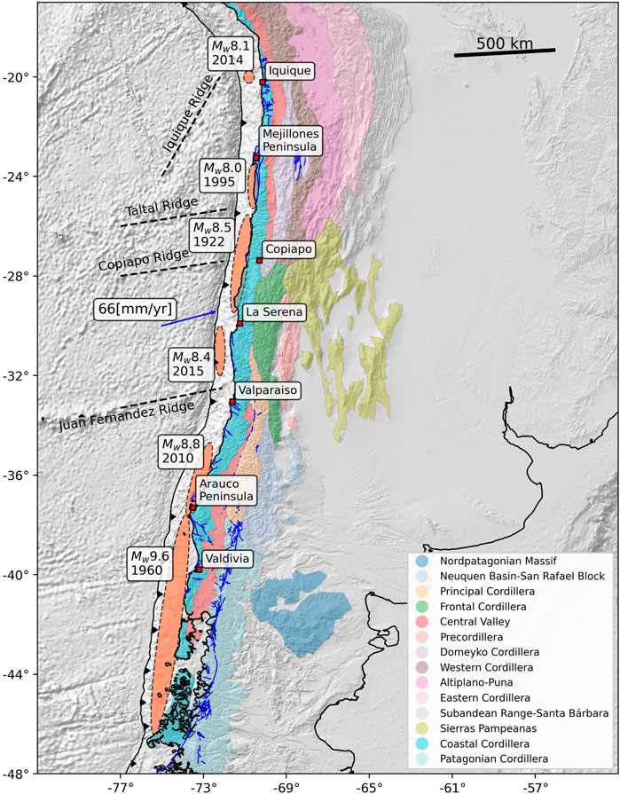
FIGURE 1. Location of the study zone. Orange ellipses represent the approximate rupture area of the earthquakes from the last 100 years in the region (Delouis et al., 1997; Beck, 1998; Ruiz et al., 2016). Red squares represent cities and relevant coastal features. Blue arrow represent the convergence velocity between Nazca and Sudamerica. Blue lines represents faults traces from (Maldonado et al., 2021). Colored regions represents the morphostructures.

Interseismic interplate coupling (e.g., Moreno et al., 2010; Wang et al., 2012; Klein et al., 2018; Becerra-Carreño et al., 2022; Yáñez-Cuadra et al., 2022) induces contraction of the upper plate that may have an influence on the long-term continental deformation. The general shapes of the short- and long-term shortening profiles are similar in the Altiplanic back-arc (e.g., Brooks et al., 2011), suggesting that the greatest strain is produced by active shortening during the interseismic period. Thus, interseismic processes may induce active continental deformation along the Andes, as observed in the movement of fore-arc rigid blocks across the Altiplano-Puna system (Figure 1) (e.g., Allmendinger et al., 2007), the regional fault systems of the Atacama Fault Zone (AFZ) in the fore-arc between 21°S and 30°S (Figure 1), and strain partitioning due to strike-slip faulting along the Liquiñe-Ofqui Fault Zone (LOFZ) (e.g., Beck, 1998; Wang et al., 2007) in the volcanic arc between 37° and 47°S (Figure 1). These fore-arc structures long precede the actual subduction, and their origin lies from the Paleozoic accretion of terranes (e.g., Ramos, 2010), to Cretacic (AFZ) (e.g., Ruthven et al., 2020) and mid-Eocene (LOFZ) (e.g., Aragón et al., 2011) tectonics. The interplay between the subduction process and the continental plate structural heterogeneity (e.g., Maksymowicz, 2015; Maksymowicz et al., 2018; Molina et al., 2020) is expressed morphologically as morphostructures (Figure 1). The morphostructures are regions characterized by a certain stratigraphic succession, a structural style, and peculiar geomorphological features that are the expression of a particular geological history. Morphostructures have more or less defined limits, being able to present a transition with neighboring geological provinces (Rolleri, 1976; Ramos, 1999). Thus, as shown by strain analysis, the morphostructures could respond differently to the strain produced by the subduction process (e.g., Rosenau et al., 2006; Allmendinger et al., 2007; Cardozo and Allmendinger, 2009).

3 Data and methodology

We apply unsupervised machine learning techniques to analyze the patterns in the crustal velocities registered by GNSS networks. Particularly, we apply clustering algorithms, where the goal is to group similar observations (instances) together into groups (clusters). There are several clustering algorithms such as Birch (Zhang et al., 1996) or K-means (Lloyd, 1982), for instance that vary in methodological aspects regarding how the clusters are formed. For this work, we choose the Agglomerative clustering algorithm implemented in sklearn-scikit (Pedregosa et al., 2011). This algorithm performs a hierarchical clustering using a bottom up approach: each observation starts in its own cluster, and clusters are successively merged together (Pedregosa et al., 2011). We use Ward’s linkage, a linkage criterion that serves as a measure of similarity between sets of observations, to decide which clusters should be merged. Thus, at each step, we test the linkage of a pair of clusters to find the pair of clusters that leads to a minimum increase in the total within-cluster variance after merging.

The Agglomerative clustering algorithm differs from other algorithms such as K-means in that it does not start with a random seed, so the clustering remains stable when re-running the clusterization. It also differs from other hierarchical algorithms, such as Birch, in that it only requires the link criterion and the number of clusters (k) as hyperparameters.

Pre-processing the data is a vital aspect of the machine learning workflow, as it helps find hidden patterns in the data and thus leads to better learning. Therefore, as input features for the Agglomerative algorithm, this study explores two methodologies based on two dataset of GNSS secular rates. The first method is based on the velocities and it is similar to those applied by Simpson et al. (2012), Savage and Simpson (2013), Thatcher et al. (2016), Granat et al. (2021). For the second method, we developed a strategy to pre-process GNSS velocities by calculating surface strain and rotational rates to generate features to be clustered with machine learning. Thus, the goal is to search for hidden patterns of the crustal motion that can be associated with the shallow crustal structure of the margin.

3.1 Dataset of GNSS secular rates

This study analyzes the surface velocity field derived from GNSS observations for two time periods. The first dataset consists of observations acquired prior to the years 2010 (24°S–45°S) and 2014 (18°S–24°S). These segments were in an interseismic phase of the seismic cycle (e.g., Klotz et al., 2001; Moreno et al., 2008; Ruegg et al., 2009) during these periods, except in the southern part where the effects of prolonged postseismic deformation from the great 1960 Valdivia earthquake were still being observed (Hu et al., 2004). Between 2010 and 2015, the Chilean margin was affected by three major earthquakes: Maule (M_w 8.8) in 2010 (Moreno et al., 2010); Iquique (M_w 8.1) in 2014 (Schurr et al., 2014; Duputel et al., 2015); and Illapel (M_w 8.2) in 2015 (Heidarzadeh et al., 2016; Tilmann et al., 2016). These events produced a large coseismic deformation as well as postseismic deformation. The second dataset considers the period 2018–2021 in which there are still areas with post-seismic effects from recent earthquakes and regions undergoing interseismic contraction (Baez et al., 2018). These two datasets allow us to investigate changes in the velocity field related to the seismic cycle of large earthquakes on a decadal scale and explore persistent patterns in surface deformation.

The pre-2014 dataset consists of a compilation of horizontal velocities from survey-mode (sGNSS) and continuous GNSS data (cGNSS) that characterize about a decade of observations. This dataset is based on the one used by Becerra-Carreño et al. (2022) but covering an area between 18°S and 45°S. The sGNSS velocities are based on the compilation of Métois et al. (2016). These include 325 sGNSS vectors published by Brooks et al. (2003), Kendrick et al. (1999), Khazaradze and Klotz (2003), Ruegg et al. (2009), Moreno et al. (2011), Métois et al. (2012), Métois et al. (2013), Weiss et al. (2016). These velocities are estimated with respect to the stable part of South America following Métois et al. (2012). We processed GNSS observations from 123 continuous stations using the processing strategy of Baez et al. (2018). From the time series of continuous station time series, we estimate horizontal velocities using the Bevis and Brown (2014) trajectory model. For the period 2018–2021, we processed all available GNSS station data (202 stations). We followed the same processing procedure and time series analysis used for the pre-2014 period cGNSS data. We transform all velocities estimated from the cGNSS time series to a stable reference frame of the South American continent by subtracting the rotational motion of a rigid plate using the Euler pole defined by Métois et al. (2012). Thus, the sGNSS and cGNSS velocities (Figure 2) are compatible since they are referenced to the same reference frame.

FIGURE 2

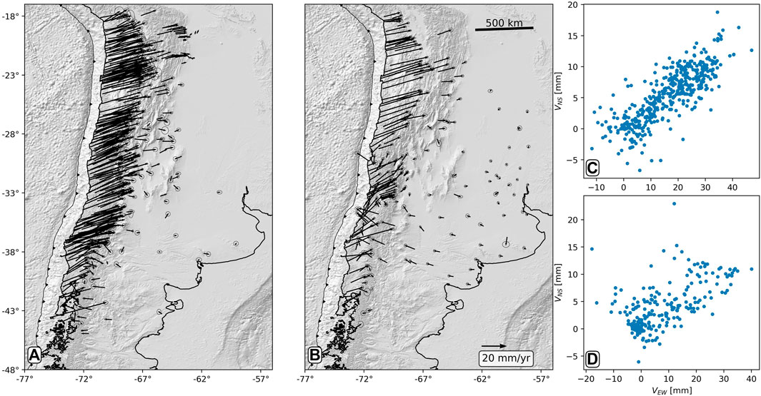
FIGURE 2. Study zone map and the GNSS interseismic velocities used in this study. (A,C) show pre-2014 velocities, and (B,D) show 2018–2021 velocities.

The pre-2014 velocity field is relatively homogeneous (Figure 2A), with most of the margin (18°S–38°S) showing typical interseismic contraction patterns, i.e., directions parallel to the plate convergence vector and magnitudes decreasing landward. In the extreme north (18°S–24°S), the deformation extends almost 500 km from the coast, with velocities that decrease drastically on the eastern slope of the Andes. This gradient has been interpreted as deformation related to crustal shortening in the back-arc margin of the Andes (e.g., Brooks et al., 2011; Weiss et al., 2016). South of 38°S, the vectors show opposite directions, i.e., the vectors near the coast move towards land, while the vectors in Argentina move towards the trench. This segment is in a late postseismic period, where interseismic compression predominates near the coast (Hu et al., 2004). In contrast, in the back-arc, there are still effects of viscoelastic relaxation induced by the 1960 earthquake, which is visible over 50 years after this event (Moreno et al., 2011). The 2018–2021 velocity field is more complex (Figure 2B), showing that different segments are in different phases of the seismic cycle. The 2010 Maule earthquake caused post-seismic deformation of continental scale, as evidenced by the trenchward vectors between 33°S and 40°S. The post-seismic effects of the Illapel earthquake are of a local scale, only affecting areas very close to the rupture zone (29°S–30°S). North of 30°S, the margin is in an interseismic period, and the effects of the 2014 earthquake are only visible as lower magnitude velocities near the rupture zone (19°S).

3.2 Velocity clustering

We start the analysis with a clustering approach using the estimated horizontal velocities of the GNSS stations straightforwardly as features. We express the directions of the horizontal velocities as their unit vector (direction of the North and East components with values between −1 and 1) and norm (magnitude), thus considering three features for each GNSS station. We show the flowchart of this methodology in the upper part of the pre-processing stage of Figure 3. These features are standardized previous to the clustering. As the number of clusters (the hyperparameter k) need to be specified beforehand, we tested 5 to 10 clusters. The criteria used to choose k is based on the competence between maximizing the number of clusters so more information can be visualized while not desegregating the data too much by having small clusters of less than ten stations. In doing so, we choose the optimal value of k for each period (Figure 4) and show the results of the other values of k in the Supplementary Material.

FIGURE 3

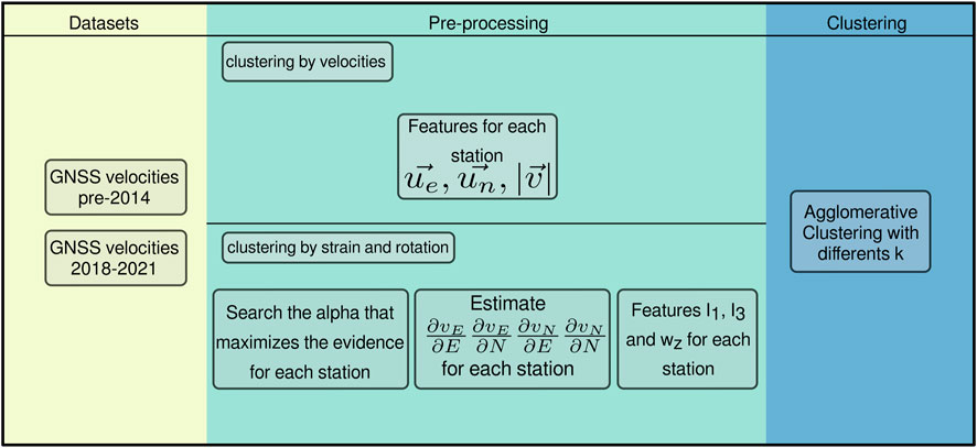
FIGURE 3. Flowchart summarizing the different stages of the clustering analysis. In a first step, the two datasets of velocities are generated from the GNSS data, then these two datasets are pre-processed using the two the methods presented in this work (i.e., clustering by velocity and strain-rotation). In a final step, the features extracted from these datasets are clustered using the Agglomerative algorithm.

FIGURE 4

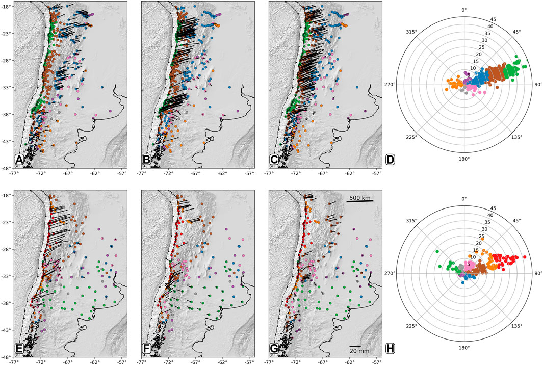
FIGURE 4. Velocity clustering results for the period pre-2014 with k = 7 (A–C) and the period 2018–2021 with k = 8 (E–G), and their respective polar representations (D,H).

3.3 Surface strain and rotation rates clustering

First, we calculate the velocity gradients from a linear expansion of the surface velocity field around a point with velocity v^o,

${\mathbf{v}}^{\mathbf{i}}={\mathbf{v}}^{\mathbf{o}}+\mathbf{L}{\mathbf{\Delta }}^{\mathbf{i}}(1)$

where ${\mathbf{v}}^{\mathbf{i}}={\left[\begin{array}{cc}\hfill v_E^i\hfill & \hfill v_N^i\hfill \end{array}\right]}^{\top }$ is the horizontal velocity measured at the i-th GNSS station, with relative location ${\mathbf{\Delta }}^{\mathbf{i}}={\left[\begin{array}{cc}\hfill {\mathrm{\Delta }}_E^i\hfill & \hfill {\mathrm{\Delta }}_N^i\hfill \end{array}\right]}^{\top }$ from the reference point with velocity ${\mathbf{v}}^{\mathbf{o}}={\left[\begin{array}{cc}\hfill v_E^o\hfill & \hfill v_N^o\hfill \end{array}\right]}^{\top }$. Here, E and N refer to the East and North directions, which define the basis vectors of the coordinate system used to describe the velocities and coordinates of the GNSS stations. L is the velocity gradient tensor, i.e., the derivatives of the velocity field with respect to Easting (E) and Northing (N). We use the method described by Cardozo and Allmendinger (2009) to estimate the reference velocity v^o and the velocity gradients L. Here, the velocity data measured at n GNSS stations to provide a constrain to the weighted least squares,

$\underset{\mathbf{m}}{\text{min}}\sum _{\mathbf{i}=1}^n{‖w_{\mathbf{i}}\left({\mathbf{G}}^{\mathbf{i}}\mathbf{m}-{\mathbf{v}}^{\mathbf{i}}\right)‖}_2^2(2)$

where Gⁱ, m and vⁱ are defined by reordering Eq. 1. In such terms, Gⁱm correspond to the velocity prediction at the i-th GNSS station (right hand side of Eq. 1), with design matrix

${\mathbf{G}}^{\mathbf{i}}=\left[\begin{array}{cccccc}\hfill 1\hfill & \hfill 0\hfill & \hfill {\mathrm{\Delta }}_E^i\hfill & \hfill {\mathrm{\Delta }}_N^i\hfill & \hfill 0\hfill & \hfill 0\hfill \\ \hfill 0\hfill & \hfill 1\hfill & \hfill 0\hfill & \hfill 0\hfill & \hfill {\mathrm{\Delta }}_E^i\hfill & \hfill {\mathrm{\Delta }}_N^i\hfill \end{array}\right](3)$

and vector of unknown parameters

$\mathbf{m}=\left[\begin{array}{cccccc}\hfill v_E^o\hfill & \hfill v_N^o\hfill & \hfill L_{EE}\hfill & \hfill L_{EN}\hfill & \hfill L_{NE}\hfill & \hfill L_{NN}\hfill \end{array}\right](4)$

where L_EE = ∂v_E/∂E, L_EN = ∂v_E/∂N, L_NE = ∂v_N/∂E and L_NN = ∂v_N/∂N are the components of the velocity gradient tensor L (e.g., Davis and Titus, 2011).

The term $w_{\mathbf{i}}=\left[\begin{array}{cc}\hfill {\sigma }_{v_E^i}^{-1}\hfill & \hfill 0\hfill \\ \hfill 0\hfill & \hfill {\sigma }_{v_N^i}^{-1}\hfill \end{array}\right]\text{exp}\left(-\frac{d}{\alpha }\right)$ is an importance weight assigned to the velocity ${\mathbf{v}}^{\mathbf{i}}={\left[\begin{array}{cc}\hfill v_E^i\hfill & \hfill v_N^i\hfill \end{array}\right]}^{\top }$, with standard deviations ${\sigma }_{v_E^i}$ and ${\sigma }_{v_N^i}$, measured at the i-th GNSS station, located at a distance d = ‖Δⁱ‖ from the reference point. Here, α is a constant that controls how quickly the weight decays with the distance from the reference point. It therefore controls the spatial scale at which strain is estimated. The velocity vⁱ of a GNSS station located at a distance α from the reference point will have a weight of 0.34 relative to a weight of 1 for a station located at the reference point (see Supplementary Figure S25). In the context of least-squares inversion, such weighting is equivalent to assigning almost three times the standard deviation (e.g., Tarantola, 2005) to such GNSS velocities. Thus, velocity gradient estimates are mostly representative of an homogeneous deformation and rotation occurring within a distance ∼ α from the reference point.

The estimated velocity gradient tensor L can be decomposed as

$\mathbf{L}=\dot{\mathit{\omega }}+\dot{\mathit{\epsilon }}(5)$

where the rotation rate tensor $\dot{\mathit{\omega }}=\frac{1}{2}(\mathbf{L}-{\mathbf{L}}^{\top })$ is the skew-symmetric part of L and represents a rotational crustal motion, while Cauchy’s strain rate tensor $\dot{\mathit{\epsilon }}=\frac{1}{2}(\mathbf{L}+{\mathbf{L}}^{\top })$ is the symmetric part of L and models surface velocities due to strain rate.

From $\dot{\mathit{\omega }}$ and $\dot{\mathit{\epsilon }}$, a set of features for the clustering algorithm are calculated. From the rotation rate tensor $\dot{\mathit{\omega }}$, we extract the vertical vorticity (e.g., Davis and Titus, 2011) as,

$w_z=2{\dot{\omega }}_{NE}=L_{NE}-L_{EN}=\frac{\partial v_N}{\partial E}-\frac{\partial v_E}{\partial N}(6)$

which indicates the magnitude and direction of the rotation (around the vertical axis z) of the surface of the crust (positive for anticlockwise rotation and negative for clockwise rotation). Using the values of the deformation rate tensor $\dot{\mathit{\epsilon }}$, we calculate the first (I₁) and third (I₃) invariants, as their values are independent of the choice of reference frame used to describe strain rates (e.g., Timoshenko and Goodier, 1951). I₁ is the trace of $\dot{\mathit{\epsilon }}$ and I₃ is the determinant of $\dot{\mathit{\epsilon }}$. The physical interpretation of I₁ is the volumetric deformation, where a positive value indicates dilatation and a negative value indicates contraction. There is no clear physical interpretation for I₃, but it differentiates from I₁ by accounting for shear strain rates. It is worth mentioning that the features are computed from velocity gradients that are in turn estimated using velocities observed at spatially nearby GNSS stations. Thus, we are indirectly adding local geographic information to the problem.

Problem (Eq. 2) can be solved to find the aforementioned features (I₁, I₃, w_z) for an arbitrary set of reference points. Typically, an homogeneous grid is used (e.g., Allmendinger et al., 2007; Cardozo and Allmendinger, 2009; Melnick et al., 2017). However, as we aim to define such features to be used in a clustering algorithm, we only estimate the features at the GNSS station locations, where the original datasets are located. In that way, we calculate one feature set per original velocity observation, avoiding generating an uneven number of features associated to each original velocity observation, due to a spatially heterogeneous distribution of the GNSS sites.

A fixed value of α must be set previous to solving the linear least squares inversion (Eq. 2) at a given reference point. Therefore, we solve the problem for a range of tentative values of α from 10 to 650 km. We choose this range of values because values below 10 results in a highly heterogeneous velocity gradient field, due to α being too similar to the shorter distances between GNSS stations. We choose a more flexible upper limit of α, since higher values could be necessary to solve the least squares problems in regions where the distance between GNSS sites is larger. Then, we select the optimum value of α as the one that maximizes the evidence of the least squares problem solution (Sambridge et al., 2006). The evidence is a mathematical model comparison method that incorporates the principle of natural parsimony. Therefore, selects the best model as the simpler one among those that fit equally well the observations, being particularly good at avoiding overfitting, i.e., selecting models that do not explain the noise in the observations. As a consequence of using the evidence to select the best value of α at each GNSS station, the spatial scale at which the features are estimated is related to the changes in density of GNSS instrument location across the network. Thus, we obtain a smoother spatial distribution of features at regions with few GNSS stations installed, and more heterogeneous feature distribution (as required by the data) at the denser parts of the GNSS network.

We apply the Agglomerative clustering algorithm to the estimated features at all GNSS station locations, and test a number of clusters from 5 to 20 clusters. As with the velocity clustering method, we leave an open discussion about the best number of clusters, and discuss how this reflects the strain and rotation distribution over the Andes. We show the flowchart of this methodology in the lower part of the pre-processing steps in Figure 3.

4 Results

4.1 Clustering by velocities

4.1.1 Period pre-2014

We show in Figure 4 the results for the clustering by velocities for k = 7 and k = 8 for period pre-2014 and 2018–2021, respectively (see Supplementary Material for results with others k). The main clusters of the period pre-2014, indicated by blue, brown and green circles in Figure 4, are associated with the variations of the interseismic velocity field within the fore-arc and back-arc. The green cluster (Figure 4B) contains the higher ($>$30 mm/yr) eastward interseismic velocities in the dataset. The brown cluster (Figure 4C) is composed of medium (∼18–30 mm/yr) interseismic velocity segments, while the blue (Figure 4A) cluster holds low ($<$18 mm/yr) eastward velocities in the back-arc and in the fore-arc south of 38°S.

The smallest clusters are the purple, orange, pink, and gray colored GNSS, which are related to local tectonics. The orange cluster (Figure 4A) is composed of westward velocities south of 38°S. The rest of the clusters for the period pre-2014 have higher velocities in the North-South direction. The pink cluster (Figure 4B) comprises back-arc velocities with a clockwise rotational component. The purple cluster (Figure 4C) is composed of back-arc velocities in the north direction. Finally, the gray cluster (Figure 4C) is composed of back-arc velocities with a southwest direction. The latter seems to be associated with the orange cluster, both affected by a clockwise rotation in the back-arc.

4.1.2 Period 2018–2021

The results for the period 2018–2021 are shown in the lower panels of Figure 4. In the fore-arc, the orange cluster (Figure 4E) is composed of interseismic northeastward velocities between 10 to ∼22 mm/yr in the fore-arc. This cluster covers areas close to the rupture zones of the Iquique M_w8.1 2014, Illapel M_w8.3 2015 and Maule M_w8.8 2010 earthquakes (e.g., Moreno et al., 2010; Lin et al., 2013; Duputel et al., 2015; Heidarzadeh et al., 2016). In turn, the red cluster represents the higher velocities in the dataset and is composed of $>22$ mm/yr northeastward velocities in the fore-arc and it is found in the seismic gaps of the Northern Chile (20°S–23°S), Atacama (23°S–28°S) and Valparaiso (32°S–33°S). Surprisingly, it is also found in the Arauco peninsula at 38°S, which ruptured in the Maule 2010 earthquake, suggesting a rapid re-coupling of this area after this event.

In the back-arc, the pink cluster (Figure 4E) is composed of northward velocities ($<$ 10 mm/yr) mainly located in the Andes at ∼32°S across the Precordillera morphostructure; this pattern of velocities was not present in this area in the period pre-2014. The green cluster (Figure 4F) represents westward velocities ($<$25 mm/yr) in the fore-arc and back-arc near the rupture zone of the Maule M_w8.8 2010 earthquake. The blue cluster (Figure 4F) is composed of southward velocities ($<$10 mm/yr). The brown cluster (Figure 4G) is composed of eastward velocities ($<15$mm/yr) in the fore-arc at 18°S and 33°S, and in the back-arc between 23°S and 28°S. The gray cluster (Figure 4G) is composed of very low ($<5$mm/yr) northwest velocities and it scatteringly distributed through the back-arc. Finally, the purple cluster (Figure 4G) is composed of very low southwestward velocities ($<5$mm/yr) and it is distributed through the back-arc.

4.2 Clustering by surface strain and rotation rates

4.2.1 Surface strain and rotation rates

Figure 5 shows the evidence values for each trial α value used to solve the least squares problem (Eq. 2) at each GNSS station location. The α values that maximize the evidence for each station range between 50 and 650 km, being mostly concentrated between 100 and 400 km for the pre-2014 dataset, and between 150 and 350 km for the 2018–2021 dataset.

FIGURE 5

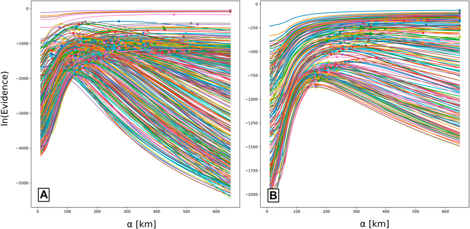
FIGURE 5. Evidence values for the least squares solution at each GNSS station (colored lines) for the range of values of α. Colored squares represent the α value that maximizes the evidence for each station. Dataset period pre-2014 (A) and dataset period 2018–2021 (B).

We show the estimated values for I₁, I₃ and w_z for both periods in Figure 6. For the period before 2014 (Figures 6A–C), these features are dominated by a long wavelength signal that becomes more heterogeneous south of 33°S. The I₁ feature distribution (Figure 6A) shows a northwest lineament in its values toward the Andes north of 35°S, and north-south and east-west variations that the clustering algorithm uses to determine data separation. In the pre-2014 period (Figure 6), a maximum contraction (Figure 6A) and clockwise rotation (Figure 6C) occur near the coast in front and to the south of the 2010 (M_w8.8) Maule earthquake rupture zone (34°S–38°S, see Figure 1), signals that decay towards the back-arc and to the north. Figure 6B also shows that there is a boundary in the sign of the I₃ values at 38°S, which coincides with the southern boundary of the 2010 Maule earthquake (M_w8.8).

FIGURE 6

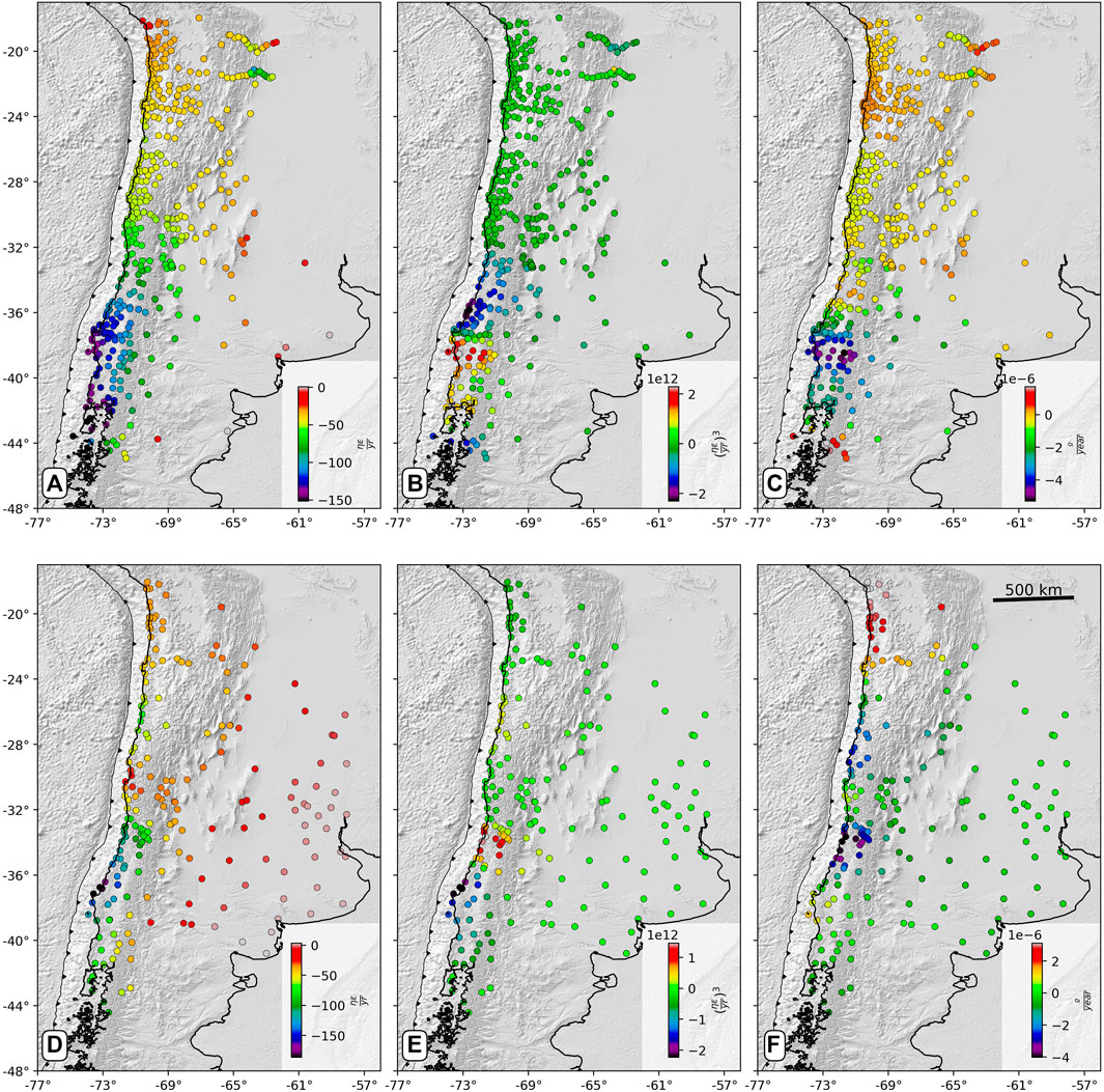
FIGURE 6. Features value. Pre-2014 I₁ (A), pre-2014 I₃ (B) and pre-2014 w_z (C), 2018–2021 I₁ (D), 2018–2021 I₃ (E) and 2018–2021 w_z (F).

The contraction signal south of 36°S of $<-100\frac{\eta \epsilon }{yr}$ (nano-strain per year) in the period before 2014 is produced by the eastward velocities $>$ 30 mm/yr (green cluster in Figure 4) in the fore-arc combined by a low velocity in the back-arc (pink and orange cluster in Figure 4). This is particularly interesting since the comparison of I₁ between both periods (Figure 7) shows that even after the 2010 Maule earthquake (M_w8.8), a higher amount of contraction is found in the 2018–2021 period in the same region. On the other hand, the contraction in the area in front of the 2014 (M_w8.2) Iquique earthquake ($\sim 20$°S) maintains an equal amount of contraction of $\sim -30\frac{\eta \epsilon }{yr}$ in both periods. Finally, in the zone in front of the 2015 (M_w8.3) Illapel earthquake (30°S–32°S), the contraction decreases from ∼ −60 to $\sim -30\frac{\eta \epsilon }{yr}$ (Figure 7), revealing a post-seismic relaxation in this region.

FIGURE 7

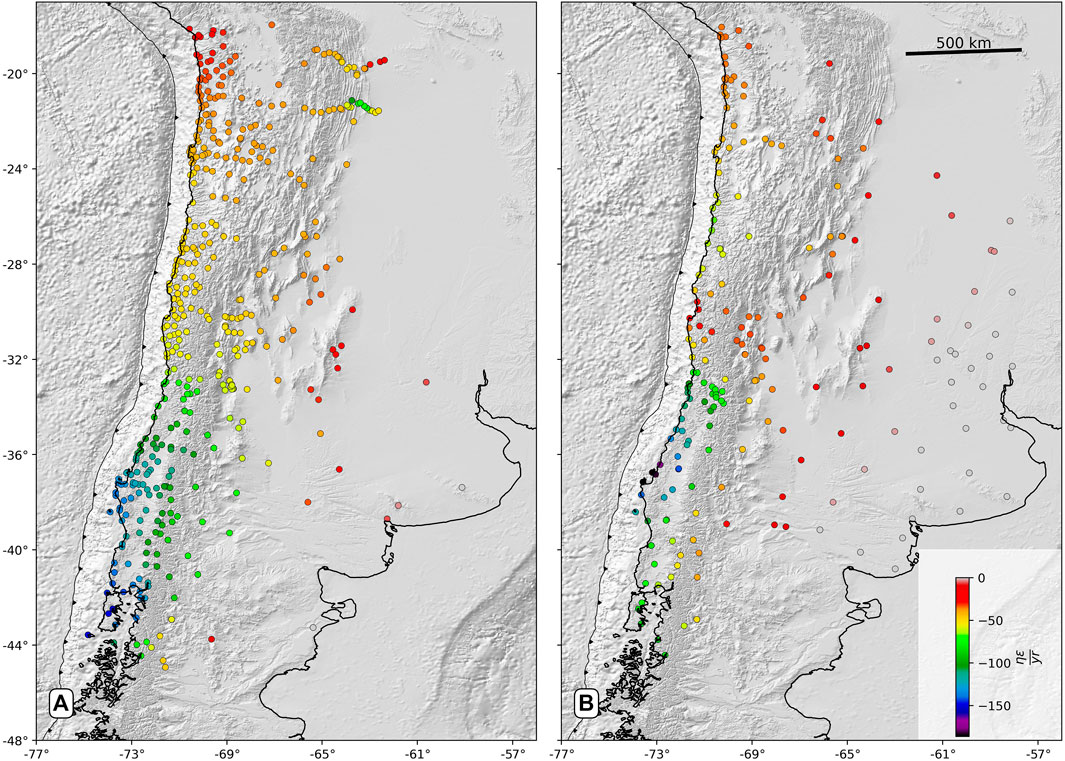
FIGURE 7. I₁ feature value for both periods colored with the same color scale. Pre-2014 (A), 2018–2021 (B).

The general decrease in the contraction occurs in almost the entire margin, even in the arc and back-arc, with three exceptions. Northward in the Valparaiso seismic gap (33°S), there is an increase in contraction from $-80\frac{\eta \epsilon }{yr}$ in the pre-2014 period to $\sim -100\frac{\eta \epsilon }{yr}$ in the 2018–2021 period (Figure 7). Here, the increase in contraction in the 2018–2021 period appears to be associated with a sharp decrease in velocities between GNSS stations in the fore-arc (red cluster in Figure 4E) and back-arc (brown cluster in Figure 4G), where velocities decrease to $<10$ mm/yr. A similar behavior occurs in the Atacama seismic gap, where there is an increase in contraction from −50 to $-80\frac{\eta \epsilon }{yr}$. Finally, the maximum increase in contraction between the periods is found at 37°S with an increase from −125 to $-175\frac{\eta \epsilon }{yr}$.

4.2.2 Clustering

We present the results of clustering by I₁, I₃ and w_z in Figure 8, showing the clustering configuration for two different number of clusters (k = 9 and k = 15) for the pre-2014 period. The results for other values of k and the cluster analysis for the period from 2018 to 2021 are presented in the supplementary material (Supplementary Figures S9–S24).

FIGURE 8

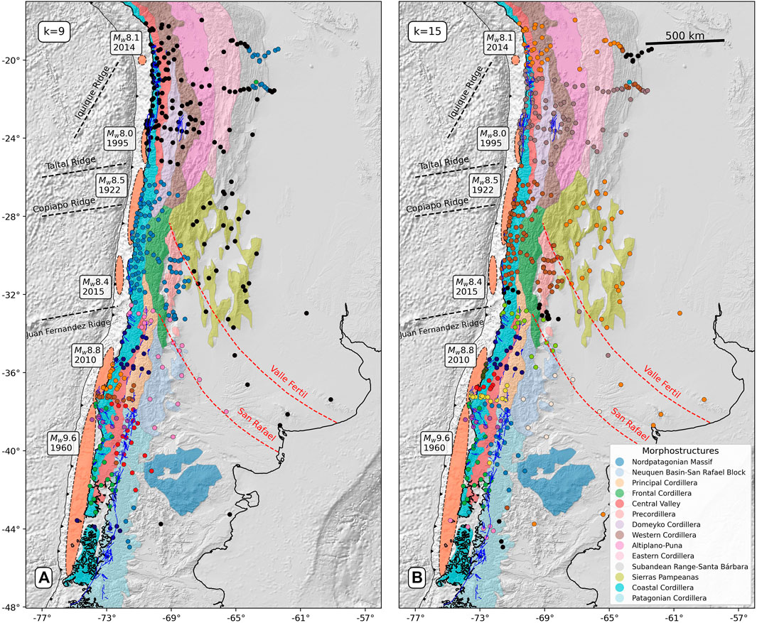
FIGURE 8. Clustering by I₁, I₃ and w_z for the period pre-2014 with k = 9 (A) and k = 15 (B). Blue lines represents faults traces from (Maldonado et al., 2021). Colored regions represents the morphostructures. Orange ellipses represent the approximate rupture area of the earthquakes from the last 100 years in the region (Delouis et al., 1997; Beck, 1998; Ruiz et al., 2016). Dotted red lines represents the Valle Fertil and San Rafael lineaments of (Jacques, 2003).

Our results suggest that the spatial distribution of the strain-based clusters in the fore-arc is correlated with the rupture zones of the earthquakes, and in turn follows a northwesterly lineament that crosses the Andes. By following these lineament, the clusters distribution correlates with some important limits of the morphostructures.

In the clustering with k = 9 (Figure 8A), it is possible to observe a first-order latitudinal separation of the clusters. This boundary is at 32°S, where the northern segment is composed by the blue and black clusters, while southern segment is composed by the pink, dark blue, orange, brown, green, red, and purple clusters. In the northern segment, two clusters follow the Valle Fertil and San Rafael northwest lineaments (Jacques, 2003). Here, the black cluster is mainly found in the Altiplano-Puna, Domeyko Cordillera, Western and Eastern Cordillera, Subandean Range and Sierras Pampeanas morphostructures. In turn, the blue cluster is found in front of the ruptures of the 1922 M_w8.5 Atacama and 2015 M_w8.4 Illapel earthquakes, and the morphostructures of the Cordillera Frontal and Precordillera. These clusters are also correlated with the disappearance of the volcanic arc between 28°S and 32°S due to the presence of the flat slab. The blue cluster is also found locally in the Subandean Range and in the Patagonian Cordillera.

The second group of clusters is located south of 33°S, where the flat slab ends and the Southern Volcanic Zone begins (Figure 8A). The pink cluster limits the first group of cluster and follows the northwest trend in northern Chile. To the south of the pink cluster, the clusters in this second group no longer follow a north-west lineament, but instead follow north-south (green and red clusters) to east west (brown cluster) lineaments. The pink and the dark blue clusters are located in the Valparaíso seismic gap. The orange-blue cluster correlates with the rupture of the 2010 (M_w8.8) Maule earthquake and coincides with the limits of the velocity-based green cluster of Figure 4. The brown and purple clusters follow an east-west lineament in the fore-arc that correlates with the boundary between the Maule and Valdivia earthquakes and the beginning of the Patagonian Cordillera. The red cluster follows a north-south lineament in the northern part of the Patagonian Cordillera, characterized by the presence of the LOFZ, which controls volcanism in the region (Cembrano and Lara, 2009). The green cluster is located in the fore-arc close to the coastline along the 1960 M_w9.5 Valdivia rupture zone. Finally, the dark blue cluster is also found in the southern part of the LOFZ. This clustering shows the effects on the strain and rotation field of the deformation processes of the seismic cycle and the possible motions in the LOFZ recorded in the GNSS displacements (e.g., Wang et al., 2007).

The highest correlation with local structures is produced when k = 15 (Figure 8B). Here, some clusters disaggregate with the increasing of k without changing the overall limits between the clusters. Following the description for each cluster, the principal differences with k = 9 lies in the division of the black cluster (Figure 8A) into the orange and light brown clusters (Figure 8B). This separation divides the structural styles of the Altiplano-Sierras Pampeanas with the Domeyko Cordillera-Puna in the arc and back-arc. The orange cluster also correlates with the rupture of the 2014 M_w8.1 Iquique earthquake from the north of Chile seismic gap and correlates with the green and brown clusters of Figures 4B, C, which shows a decrease in interseismic velocities at 20°S. Another good correlation, occurs in the division of the blue cluster (Figure 8A) at ∼32°S into the brown and black clusters (Figure 8B), which continue the expression of the northwest lineament of the nearby clusters. In the same region, the pink cluster (Figure 8A) is divided into the light green and the white clusters in the southern part of the Neuquen Basin (Figure 8B). The dark blue cluster (Figure 8A) splits into the dark blue and pink clusters at 44°S (Figure 8A). Finally, the clusters with less morphostructural spatial correlation are found in front of the Maule M_w8.8 earthquake. Here, the orange cluster (Figure 8A) is divided into the dark brown and red clusters. A similar case is the green cluster (Figure 8A) that is divided into the green and the light blue clusters in the Subandean Range (Figure 8B) and on the coast at 43°S.

5 Discussion

The two analyses based on velocities and strain/rotation rates indicate that GNSS velocity clustering provides a tool for characterizing active deformation patterns on a local to regional scales. While velocity-based clustering helps to assess the different deformation patterns of the seismic cycle, an increase in complexity using strain rate invariants and rotation rates as features reveals clusters associated with the Andean morphostructures, uncovering segmentations hidden in the GNSS-derived velocity field. The selection of two time periods of GNSS observations proved helpful in verifying the spatial extent of deformation changes due to postseismic effects and in exploring the stable patterns between these two periods. However, a limitation of this work is the determination of the optimal value of k, which affects the number of clusters. While functions such as the Sillhuete or the Calinski-Harabasz scores exist to determine the optimal value of k in unsupervised learning, we found inconsistent results when testing these functions. After extensive testing (see Supplementary Material S3–S24), we chose the optimal k based on a visual inspection of the results, and we decided on a number of clusters that did not overfit the observations (k < 10 for velocity clustering and k < 16 for strain and rotational clustering).

5.1 Velocity clustering

Previous studies (Simpson et al., 2012; Thatcher et al., 2016; Granat et al., 2021) found a direct relationship between the velocity clustering and style of deformation related to the San Andreas strike-slip fault system in Nevada. But when applying a similar methodology to the Chilean subduction zone, the results show instead the patterns of seismic cycle deformation (interseismic, postseismic, and back-arc shortening) at a regional to continental scale. It demonstrates that the megathrust seismic cycle induces the main patterns of active deformation in Chile. Here, the velocity measurements may conceal smaller-scale deformation of very low magnitude (a few mm/yr) related to shallow crustal faults. This can explain why the links between GNSS velocities and crustal fault displacement have only been found locally (Moreno et al., 2008; Brooks et al., 2011; Weiss et al., 2016; McFarland et al., 2017) in the Andes.

Among the patterns we found, one of the most interesting is the segmentation by the magnitude of the eastward interseismic velocities. Given that higher coupled seismic interface segments generate higher eastward fore-arc velocities (e.g., Moreno et al., 2010; Klein et al., 2018; Yáñez-Cuadra et al., 2022); we can relate this segmentation to variations in the degree of coupling along the Chilean margin. Nevertheless, this is only applicable if we analyze segments in the same phase of the seismic cycle and assume no significant heterogeneities in the physical media, such as subducted ridges or rheological variations in the upper plate (Tassara et al., 2016; Molina et al., 2020). Therefore, some variations between segments with similar patterns may be related to the effects of rheological heterogeneities (e.g., Li et al., 2017; Itoh et al., 2021).

It has been proposed that the subduction of irregular oceanic structures, such as ridges, would promote interseismic aseismic slip and hence a less coupled interface (Wang and Bilek, 2014). This decrease in the interseismic velocities is observable in the clustering of the pre-2014 data in areas where the ridges of Iquique, Copiapo, and Juan Fernandez subduct (Figure 4). The only exception is the subduction of the Taltal Ridge. Nevertheless, recent coupling models in the region of Atacama (Yáñez-Cuadra et al., 2022) find no decrease of coupling associated with the subduction of the Taltal ridge.

The lower velocities in Valdivia observed in the pre-2014 dataset could be explained by the prolonged postseismic deformation after the 1960 giant earthquake (e.g., Hu et al., 2004). As has been shown by GNSS-derived postseismic displacements (Hu et al., 2004; Moreno et al., 2011; Klein et al., 2016; Melnick et al., 2017), rotational movements in the fore-arc could be associated with a postseismic response of the viscoelastic mantle. This effect can explain the southward velocity component in the back-arc represented by the gray and pink clusters (Figure 4A). Moreover, the clusters shown in Figure 4 indicate that the velocity patterns in the fore-arc at south of 38°S are similar to those in the back-arc north of 38°S. The velocities in this region are significantly slower than the rest of the margin. Toward the Andes, the eastward velocities decrease rapidly to the point where displacements in the back-arc change direction to westward. As shown in Li et al. (2015); Shi et al. (2020); Yáñez-Cuadra et al. (2022), the phenomenon of overlapping between deformation caused by viscoelastic and elastic processes could mislead the modeling and interpretation of GNSS observations. Moreno et al. (2011) found a late viscoelastic response from the 1960 M_w 9.5 Valdivia earthquake that affects not only the back-arc westward velocities, but also the fore-arc, where most of the interseismic deformation produced by subduction interplate coupling occurs. As interplate coupling produces eastward dominated motion on the overriding plate, a highly coupled subduction interface could be hidden by apparently slow fore-arc velocities due to such competing processes.

5.2 Surface strain and rotation rates clustering

Because we infer the features at each GNSS site using information from the neighboring stations, we indirectly introduce a geographical bias into the clustering results. This raises the question: are the resulting clusters influenced by the spatial distribution of the GNSS instruments, or are they mainly driven by their velocity observations? To validate our results, we perform a clustering based only on the location (latitude and longitude) of the GNSS stations for k = 9 and k = 15 (see Supplementary Material S1, S2). The results of the exercise show that only in a few cases the clustering by strain invariants/rotation rates and the clustering by geographical position outcomes match. This is at ∼21°S and ∼25°S in the fore-arc (k = 9 and k = 15) and at ∼30°S in the back-arc. We also test the relevance of each feature in the clustering, by converting the unsupervised clustering problem into a supervised classification problem using a random forest classifier (Ho, 1995). This is achieved by training a classifier to discriminate between each cluster and then extracting the feature importance from the model. The relevance of the features for k = 9 and k = 15 is I₁ = 0.38, w_z = 0.35, I₃ = 0.27, and I₁ = 0.37, w_z = 0.35, I₃ = 0.27 respectively. Thus, showing that the three calculated features are relevant to the clustering process.

We highlight the application of the evidence to determine the α value used to estimate the clustering features at each GNSS station. The value of α defines the weights of the velocities of nearby GNSS stations used to constrain the velocity gradient tensor (L)—and therefore the features used for clustering—when solving the least squares problem (Eq. 2). Typically, a single value of α has been used for the whole GNSS network (e.g., Allmendinger et al., 2007; Melnick et al., 2017). However, such approach does not account for the heterogeneous spatial distribution of the stations in the GNSS network. Instead, in this study we determine a different α value for each GNSS station when estimating its features. By maximizing the evidence, our method seeks to find the best α based on the parsimony principle, balancing measures of data misfits, as well as uncertainties of data and estimated parameters. Those uncertainties depend - in particular - on the relative locations of the involved GNSS stations. Thus, our work presents an improved methodology to estimate L at each GNSS station, that accounts for the spatial heterogeneity of the GNSS network. As an example, Figure 6 shows that in each period the features I₁, I₃ and w_z can be estimated with sharper spatial variations at the denser parts of the GNSS network. Additionally, the spatial scales that define the variations of the features used for clustering (Figure 6) are of the order of hundreds of kilometers. These scales are similar to those of the deformation patterns produced by the governing sources in the margin: interplate interseismic deformation, viscoelastic deformation and back-arc shortening. Between these sources of deformation, the interplate interseismic deformation presents smooth spatial variations (e.g., Métois et al., 2016; McFarland et al., 2017), and even the viscoelastic deformation is usually modeled using linear viscoelastic models (Li et al., 2017) that can sometimes be approximated by a linearly varying model (Yáñez-Cuadra et al., 2022). But even in the case of a more complex scenario with velocities presenting a less smooth spatial pattern, α values determined by the evidence should be lower since the evidence follows the principle of parsimony, with resulting features that can be lately clustered.

The visualization of the velocities, rotation rates, strain rates and their invariants (Figures 2, 6) sometimes can be useful to find spatial patterns in them. However, more subtle patterns may not be clearly visible by the naked eye. Particularly for our study, the proposed clusterization analysis is useful to elucidate patterns of strain concealed within the GNSS velocities. Additionally, such an approach eliminates the possibility of inconsistencies due to personal biases that may appear as the result of a mere visual inspection of such features.

Ideally, GNSS observations can be used to improve our understanding of the underlying physical processes by finding and interpreting a quantitative physical model able to predict such observations. Nevertheless, such physical models are often an approximation of the true physics, limited by the current knowledge and computational capabilities. Here, the clusterization analysis provides a powerful statistical tool to identify key characteristics of the data and qualitatively relate these with current knowledge without an explicit modeling of the causative physics. Therefore, we focus on analyzing the relations found between the clusterization of the features computed from GNSS data and the physical and geological aspects currently known about the subduction environmnet at the study area.

The proposed seismic segmentation of Molina et al. (2020) concludes that there is a correlation between the extent of large earthquakes and anomalous structural features of both converging plates. Thus, faults and geological composition could play a role in the diffusion of convergence induced stress in the crust, which in turn could be reflected in the crustal strain patterns. We visualize that clusterized strain and rotation rates in the fore-arc are correlated with the extent of earthquake ruptures. The boundaries between such clusters extend to the arc and back-arc along the long-term northwest-trending lineaments of the structural discontinuities (e.g., Ramos et al., 2002; Jacques, 2003). These lineaments show evidence of neotectonic activity (Ortiz et al., 2015; Perucca et al., 2018; Rothis et al., 2019) and are related to three limits between the clusters shown in Figure 8A. The first one is the northwest lineament of Valle Fertil, expressed by the boundary between the black and blue clusters (Figure 8A). The projection of this lineament continues roughly to the fore-arc. This division expresses the difference between the structural domains of the Sierras Pampeanas and Precordillera, the Frontal Cordillera and Western Cordillera, and with the northern boundary of the 1922 M_w8.5 earthquake in the fore-arc.

The second limit is the northwest lineament of San Rafael that is expressed by the boundary between the blue and pink clusters (Figure 8A). This limit in the arc is related to the difference between the structural domains of the Frontal Cordillera and Principal Cordillera, and also to the transition between the Central and Southern Andes. To the fore-arc, the continuation of the lineament coincides with the southern boundary of the 2015 M_w 8.4 earthquake. On the side of the Nazca Plate, this point also marks the change in the continental wedge, which is characterized, between Arica (∼20°S) and the subduction of the Juan Fernández Ridge (∼32°S), as an erosive margin, as evidenced by the low trench sedimentation, the absence of the accretionary prism, and a steep slope (Maksymowicz, 2015).

Finally, further south (∼37°S), the third limit is marked by the presence of the blue cluster in Figure 8B, which resembles the northern section of the trace of the LOFZ in the Patagonian Cordillera. The Patagonian Cordillera is characterized not only by the presence of the LOFZ, but also by the North Patagonian Batholith, given its basement composition (e.g., Echaurren et al., 2016) and by its role controlling the volcanism in the Southern Volcanic Zone of the Andes (Cembrano and Lara, 2009).

6 Conclusion

Our work highlights the power of combining optimization and machine learning methods to better understand the strain and rotation patterns in the subduction margin and their interplay with the geology and long term structural domains. We start by applying a clustering approach—similar to that used by other authors—to study the velocity distribution of the GNSS-network in the Chilean subduction margin. In the process, we developed a novel methodology to estimate crustal surface strain and rotations (rates) that accounts for the spatial heterogeneities of the GNSS network.

The velocity clustering results indicate a first order relation to the phases of the seismic cycle, delineating regions with different patterns of postseismic and interseismic deformation. On the other hand, clustering based on strain invariants and rotation rates, shows a link between the seismic segmentation in the fore-arc and the geological and structural domains in the arc and back-arc. The latter can be recognized by the clusters associated with different morphostructures and cluster boundaries similar to the northwest lineaments of structural discontinuities.

Data availability statement

The raw data supporting the conclusion of this article is available by at https://github.com/VicenteYanez/gnss-strain-clustering Further enquires can should be directed to the corresponding author.

Author contributions

VY-C and MM conceived the original idea of this study with the contribution of FO-C. FO-C adapted the evidence mathematical framework to the strain and rotation analysis. VY-C developed the computational codes with the contribution of FO-C. VY-C performed the analysis. JB and MM processed the GNSS data. FD contribute in the machine learning verification of the result. AT contribute in the tectonic analysis and interpretation of the results. VY-C, MM, and FO-C wrote the article with contributions from the other authors.

Funding

The authors receive funding from the following agencies: FD, JB, MM, FO-C, and VY-C—PIA-ACT192169 AT—Millenium Nucleus CYCLO-NC160025; this publication is partially funded by FONDECYT Project 1221507, ANID.

Acknowledgments

FD, JB, MM, FO-C, and VY-C acknowledge support from PIA-ACT192169 ANID Project. MM acknowledges support from FONDECYT 1221507 project. AT acknowledges support from Millenium Nucleus CYCLO-NC160025. FO-C acknowledges support from Proyecto Fondecyt 1200679 ANID. FO-C and MM acknowledge the Kobe University Strategic International Collaborative Research Grant (Type B Fostering Joint Research). We thank Shoichi Yoshioka for his comments and support for this work. FD and MM acknowledges support from IMO ICN12_019.

Conflict of interest

The authors declare that the research was conducted in the absence of any commercial or financial relationships that could be construed as a potential conflict of interest.

Publisher’s note

All claims expressed in this article are solely those of the authors and do not necessarily represent those of their affiliated organizations, or those of the publisher, the editors and the reviewers. Any product that may be evaluated in this article, or claim that may be made by its manufacturer, is not guaranteed or endorsed by the publisher.

Supplementary material

The Supplementary Material for this article can be found online at: https://www.frontiersin.org/articles/10.3389/feart.2023.1096238/full#supplementary-material

References

Allmendinger, R. W., Reilinger, R., and Loveless, J. (2007). Strain and rotation rate from GPS in tibet, anatolia, and the Altiplano. Tectonics 26, 1–18. doi:10.1029/2006TC002030

CrossRef Full Text | Google Scholar

Altamimi, Z., Rebischung, P., Métivier, L., and Collilieux, X. (2016). ITRF2014: A new release of the international terrestrial reference frame modeling nonlinear station motions. J. Geophys. Res. Solid Earth 121, 6109–6131. doi:10.1002/2016JB013098

CrossRef Full Text | Google Scholar

Aragón, E., D’Eramo, F., Castro, A., Pinotti, L., Brunelli, D., Rabbia, O., et al. (2011). Tectono-magmatic response to major convergence changes in the North Patagonian suprasubduction system; the Paleogene subduction–transcurrent plate margin transition. Tectonophysics 509, 218–237. doi:10.1016/j.tecto.2011.06.012

CrossRef Full Text | Google Scholar

Baez, J. C., Leyton, F., Troncoso, C., del Campo, F., Bevis, M., Vigny, C., et al. (2018). The chilean gnss network: Current status and progress toward early warning applications. Seismol. Res. Lett. 89, 1546–1554. doi:10.1785/0220180011

CrossRef Full Text | Google Scholar

Becerra-Carreño, V., Crempien, J. G. F., Benavente, R., and Moreno, M. (2022). Plate-locking, uncertainty estimation and spatial correlations revealed with a bayesian model selection method: Application to the central Chile subduction zone. J. Geophys. Res. Solid Earth 127, e2021JB023939. doi:10.1029/2021JB023939

CrossRef Full Text | Google Scholar

Beck, M. E. (1998). On the mechanism of crustal block rotations in the central Andes. Tectonophysics 299, 75–92. doi:10.1016/S0040-1951(98)00199-1

CrossRef Full Text | Google Scholar

Bedford, J., Moreno, M., Li, S., Oncken, O., Baez, J. C., Bevis, M., et al. (2016). Separating rapid relocking, afterslip, and viscoelastic relaxation: An application of the postseismic straightening method to the maule 2010 cgps. J. Geophys. Res. Solid Earth 121, 7618–7638. doi:10.1002/2016JB013093

CrossRef Full Text | Google Scholar

Bedford, J. R., Moreno, M., Deng, Z., Oncken, O., Schurr, B., John, T., et al. (2020). Months-long thousand-kilometre-scale wobbling before great subduction earthquakes. Nature 580, 628–635. doi:10.1038/s41586-020-2212-1

PubMed Abstract | CrossRef Full Text | Google Scholar

Bevis, M., and Brown, A. (2014). Trajectory models and reference frames for crustal motion geodesy. J. Geodesy 88, 283–311. doi:10.1007/s00190-013-0685-5

CrossRef Full Text | Google Scholar

Brooks, B. A., Bevis, M., Maturana, R., Manceda, R., Araujo, M., Smalley, R., et al. (2003). Crustal motion in the southern andes (26°-36°S): Do the andes behave like a microplate? Geochem. Geophys. Geosystems 4, 1–14. doi:10.1029/2003gc000505

CrossRef Full Text | Google Scholar

Brooks, B. A., Bevis, M., Whipple, K., Ramon Arrowsmith, J., Foster, J., Zapata, T., et al. (2011). Orogenic-wedge deformation and potential for great earthquakes in the central Andean backarc. Nat. Geosci. 4, 380–383. doi:10.1038/ngeo1143

CrossRef Full Text | Google Scholar

Cardozo, N., and Allmendinger, R. W. (2009). Sspx: A program to compute strain from displacement/velocity data. Comput. Geosciences 35, 1343–1357. doi:10.1016/j.cageo.2008.05.008

CrossRef Full Text | Google Scholar

Cembrano, J., and Lara, L. (2009). The link between volcanism and tectonics in the southern volcanic zone of the Chilean andes: A review. Tectonophysics 471, 96–113. doi:10.1016/j.tecto.2009.02.038

CrossRef Full Text | Google Scholar

Comte, D., and Pardo, M. (1991). Reappraisal of great historical earthquakes in the northern Chile and southern Peru seismic gaps. Nat. Hazards 4, 23–44. doi:10.1007/BF00126557

CrossRef Full Text | Google Scholar

Davis, J. R., and Titus, S. J. (2011). Homogeneous steady deformation: A review of computational techniques. J. Struct. Geol. 33, 1046–1062. doi:10.1016/j.jsg.2011.03.001

CrossRef Full Text | Google Scholar

Delouis, B., Monfret, T., Dorbath, L., Pardo, M., Rivera, L., Comte, D., et al. (1997). The M_w = 8.0 antofagasta (northern Chile) earthquake of 30 july 1995: A precursor to the end of the large 1877 gap. Bull. Seismol. Soc. Am. 87. doi:10.1785/BSSA0870020427

CrossRef Full Text | Google Scholar

Dong, D., Fang, P., Bock, Y., Webb, F., Prawirodirdjo, L., Kedar, S., et al. (2006). Spatiotemporal filtering using principal component analysis and Karhunen-Loeve expansion approaches for regional GPS network analysis. J. Geophys. Res. Solid Earth 111, 1978–2012. doi:10.1029/2005jb003806

CrossRef Full Text | Google Scholar

Duputel, Z., Jiang, J., Jolivet, R., Simons, M., Rivera, L., Ampuero, J. P., et al. (2015). The Iquique earthquake sequence of April 2014: Bayesian modeling accounting for prediction uncertainty. Geophys. Res. Lett. 42, 7949–7957. doi:10.1002/2015GL065402

CrossRef Full Text | Google Scholar

Echaurren, A., Folguera, A., Gianni, G., Orts, D., Tassara, A., Encinas, A., et al. (2016). Tectonic evolution of the North Patagonian Andes (41°–44° S) through recognition of syntectonic strata. Tectonophysics 677-678, 99–114. doi:10.1016/j.tecto.2016.04.009

CrossRef Full Text | Google Scholar

Géron, A. (2019). Hands-on machine learning with scikit-learn, keras, and TensorFlow: Concepts, tools, and techniques to build intelligent systems. California, United States: O’Reilly Media.

Google Scholar

Granat, R., Donnellan, A., Heflin, M., Lyzenga, G., Glasscoe, M., Parker, J., et al. (2021). Clustering analysis methods for gnss observations: A data-driven approach to identifying California’s major faults. Earth Space Sci. 8, e2021EA001680. doi:10.1029/2021EA001680

PubMed Abstract | CrossRef Full Text | Google Scholar

Heidarzadeh, M., Murotani, S., Satake, K., Ishibe, T., and Gusman, A. R. (2016). Source model of the 16 September 2015 Illapel, Chile,M_w8.4 earthquake based on teleseismic and tsunami data. Geophys. Res. Lett. 43, 643–650. doi:10.1002/2015GL067297

CrossRef Full Text | Google Scholar

Ho, T. K. (1995). “Random decision forests,” in Proceedings of 3rd international conference on document analysis and recognition, Montreal, QC, Canada, 14-16 August 1995 (IEEE).

Google Scholar

Hu, Y., Wang, K., He, J., Klotz, J., and Khazaradze, G. (2004). Three-dimensional viscoelastic finite element model for postseismic deformation of the great 1960 Chile earthquake. J. Geophys. Res. Solid Earth 109, B12403. doi:10.1029/2004JB003163

CrossRef Full Text | Google Scholar

Isacks, B. L. (1988). Uplift of the central andean plateau and bending of the Bolivian orocline. J. Geophys. Res. 93, 3211–3231. doi:10.1029/JB093iB04p03211

CrossRef Full Text | Google Scholar

Itoh, Y., Nishimura, T., Wang, K., and He, J. (2021). New megathrust locking model for the southern kurile subduction zone incorporating viscoelastic relaxation and non-uniform compliance of upper plate. J. Geophys. Res. Solid Earth 126. doi:10.1029/2020JB019981

CrossRef Full Text | Google Scholar

Jacques, J. (2003). A tectonostratigraphic synthesis of the sub-andean basins: Implications for the geotectonic segmentation of the andean belt. J. Geol. Soc. 160, 687–701. doi:10.1144/0016-764902-088

CrossRef Full Text | Google Scholar

Kendrick, E. C., Bevis, M., Smalley, R., Cifuentes, O., and Galban, F. (1999). Current rates of convergence across the central andes: Estimates from continuous gps observations. Geophys. Res. Lett. 26, 541–544. doi:10.1029/1999gl900040

CrossRef Full Text | Google Scholar

Khasraji-Nejad, H., Kahoo, A. R., Monfared, M. S., Radad, M., and Khayer, K. (2021). Proposing a new strategy in multi-seismic attribute combination for identification of buried channel. Mar. Geophys. Res. 42, 35–23. doi:10.1007/s11001-021-09458-6

CrossRef Full Text | Google Scholar

Khazaradze, G., and Klotz, J. (2003). Short- and long-term effects of GPS measured crustal deformation rates along the south central Andes. J. Geophys. Res. Solid Earth 108, 1–15. doi:10.1029/2002jb001879

CrossRef Full Text | Google Scholar

Klein, E., Fleitout, L., Vigny, C., and Garaud, J. (2016). Afterslip and viscoelastic relaxation model inferred from the large-scale post-seismic deformation following the 2010 Mw 8.8 Maule earthquake (Chile). Geophys. J. Int. 205, 1455–1472. doi:10.1093/gji/ggw086

CrossRef Full Text | Google Scholar

Klein, E., Meneses, G., Vigny, C., and Delorme, A. (2018). Bridging the gap between North and central Chile: Insight from new gps data on coupling complexities and the andean sliver motion. Geophys. J. Int. 213, 1924–1933. doi:10.1093/gji/ggy094

CrossRef Full Text | Google Scholar

Klotz, J., Khazaradze, G., Angermann, D., Reigber, C., Perdomo, R., and Cifuentes, O. (2001). Earthquake cycle dominates contemporary crustal deformation in Central and Southern Andes. Earth Planet. Sci. Lett. 193, 437–446. doi:10.1016/S0012-821X(01)00532-5

CrossRef Full Text | Google Scholar

Lange, D., Bedford, J. R., Moreno, M., Tilmann, F., Baez, J. C., Bevis, M., et al. (2014). Comparison of postseismic afterslip models with aftershock seismicity for three subduction-zone earthquakes: Nias 2005, Maule 2010 and Tohoku 2011. Geophys. J. Int. 199, 784–799. doi:10.1093/gji/ggu292

CrossRef Full Text | Google Scholar

Li, S., Moreno, M., Bedford, J., Rosenau, M., Heidbach, O., Melnick, D., et al. (2017). Postseismic uplift of the andes following the 2010 maule earthquake: Implications for mantle rheology. Geophys. Res. Lett. 44, 1768–1776. doi:10.1002/2016gl071995

CrossRef Full Text | Google Scholar

Li, S., Moreno, M., Bedford, J., Rosenau, M., and Oncken, O. (2015). Revisiting viscoelastic effects on interseismic deformation and locking degree: A case study of the Peru-north Chile subduction zone. J. Geophys. Res. Solid Earth 120, 4522–4538. doi:10.1002/2015JB011903

CrossRef Full Text | Google Scholar

Lin, Y.-n. N., Sladen, A., Ortega-Culaciati, F., Simons, M., Avouac, J.-P., Fielding, E. J., et al. (2013). Coseismic and postseismic slip associated with the 2010 maule earthquake, Chile: Characterizing the arauco peninsula barrier effect. J. Geophys. Res. Solid Earth 118, 3142–3159. doi:10.1002/jgrb.50207

CrossRef Full Text | Google Scholar

Lloyd, S. (1982). Least squares quantization in pcm. IEEE Trans. Inf. Theory 28, 129–137. doi:10.1109/TIT.1982.1056489

CrossRef Full Text | Google Scholar

Lomnitz, C. (2004). Major earthquakes of Chile: A historical survey, 1535-1960. Seismol. Res. Lett. 75, 368–378. doi:10.1785/gssrl.75.3.368

CrossRef Full Text | Google Scholar

Mafakheri, J., Kahoo, A. R., Anvari, R., Mohammadi, M., Radad, M., and Monfared, M. S. (2022). Expand dimensional of seismic data and random noise attenuation using low-rank estimation. IEEE J. Sel. Top. Appl. Earth Observations Remote Sens. 15, 2773–2781. doi:10.1109/JSTARS.2022.3162763

CrossRef Full Text | Google Scholar

Mahdavi, A., Kahoo, A. R., Radad, M., and Monfared, M. S. (2021). Application of the local maximum synchrosqueezing transform for seismic data. Digit. Signal Process. 110, 102934. doi:10.1016/J.DSP.2020.102934

CrossRef Full Text | Google Scholar

Maksymowicz, A., Ruiz, J., Vera, E., Contreras-Reyes, E., Ruiz, S., Arraigada, C., et al. (2018). Heterogeneous structure of the Northern Chile marine forearc and its implications for megathrust earthquakes. Geophys. J. Int. 215, 1080–1097. doi:10.1093/gji/ggy325

CrossRef Full Text | Google Scholar

Maksymowicz, A. (2015). The geometry of the chilean continental wedge: Tectonic segmentation of subduction processes off Chile. Tectonophysics 659, 183–196. doi:10.1016/j.tecto.2015.08.007

CrossRef Full Text | Google Scholar

Maldonado, V., Contreras, M., and Melnick, D. (2021). A comprehensive database of active and potentially-active continental faults in Chile at 1: 25,000 scale. Sci. data 8, 20–13. doi:10.1038/s41597-021-00802-4

PubMed Abstract | CrossRef Full Text | Google Scholar

McFarland, P. K., Bennett, R. A., Alvarado, P., and DeCelles, P. G. (2017). Rapid geodetic shortening across the eastern Cordillera of NW Argentina observed by the puna-andes GPS array. J. Geophys. Res. Solid Earth 122, 8600–8623. doi:10.1002/2017JB014739

CrossRef Full Text | Google Scholar

Melnick, D., Moreno, M., Quinteros, J., Baez, J. C., Deng, Z., Li, S., et al. (2017). The super-interseismic phase of the megathrust earthquake cycle in Chile. Geophys. Res. Lett. 784, 784–791. doi:10.1002/2016GL071845

CrossRef Full Text | Google Scholar

Métois, M., Socquet, A., Vigny, C., Carrizo, D., Peyrat, S., Delorme, A., et al. (2013). Revisiting the North Chile seismic gap segmentation using GPS-derived interseismic coupling. Geophys. J. Int. 194, 1283–1294. doi:10.1093/gji/ggt183

CrossRef Full Text | Google Scholar

Métois, M., Socquet, A., and Vigny, C. (2012). Interseismic coupling, segmentation and mechanical behavior of the central Chile subduction zone. J. Geophys. Res. Solid Earth 117. doi:10.1029/2011JB008736

CrossRef Full Text | Google Scholar

Métois, M., Vigny, C., and Socquet, A. (2016). Interseismic coupling, megathrust earthquakes and seismic swarms along the Chilean subduction zone (38°–18°S). Pure Appl. Geophys. 173, 1431–1449. doi:10.1007/s00024-016-1280-5

CrossRef Full Text | Google Scholar

Minson, S. E., Simons, M., and Beck, J. L. (2013). Bayesian inversion for finite fault earthquake source models I—Theory and algorithm. Geophys. J. Int. 194, 1701–1726. doi:10.1093/gji/ggt180

CrossRef Full Text | Google Scholar

Molina, D., Tassara, A., Melnick, D., Abarca del Rio, R., and Madella, A. (2020). Frictional segmentation of the chilean megathrust from a multivariate analysis of geophysical, geological and geodetic data. Earth Space Sci. Open Archive 37, 10503796. doi:10.1002/essoar.10503796.1

CrossRef Full Text | Google Scholar

Moreno, M., Melnick, D., Rosenau, M., Bolte, J., Klotz, J., Echtler, H., et al. (2011). Heterogeneous plate locking in the south–central Chile subduction zone: Building up the next great earthquake. Earth Planet. Sci. Lett. 305, 413–424. doi:10.1016/j.epsl.2011.03.025

CrossRef Full Text | Google Scholar

Moreno, M., Rosenau, M., and Oncken, O. (2010). 2010 Maule earthquake slip correlates with pre-seismic locking of Andean subduction zone. Nature 467, 198–202. doi:10.1038/nature09349

PubMed Abstract | CrossRef Full Text | Google Scholar

Moreno, M. S., Klotz, J., Melnick, D., Echtler, H., and Bataille, K. (2008). Active faulting and heterogeneous deformation across a megathrust segment boundary from gps data, south central Chile (36–39°s). Geochem. Geophys. Geosystems 9. doi:10.1029/2008GC002198

CrossRef Full Text | Google Scholar

Mousavi, J., Radad, M., Monfared, M. S., and Kahoo, A. R. (2022). Fault enhancement in seismic images by introducing a novel strategy integrating attributes and image analysis techniques. Pure Appl. Geophys. 179, 1645–1660. doi:10.1007/s00024-022-03014-y

CrossRef Full Text | Google Scholar

Nasri, S., Kalate, A. N., Kahoo, A. R., and Monfared, M. S. (2020). New insights into the structural model of the makran subduction zone by fusion of 3d inverted geophysical models. J. Asian Earth Sci. 188, 104075. doi:10.1016/J.JSEAES.2019.104075

CrossRef Full Text | Google Scholar

Ortega-Culaciati, F., Simons, M., Ruiz, J., Rivera, L., and Díaz-Salazar, N. (2021). An EPIC tikhonov regularization: Application to quasi-static fault slip inversion. J. Geophys. Res. Solid Earth 126, 1–20. doi:10.1029/2020JB021141

CrossRef Full Text | Google Scholar

Ortiz, G., Alvarado, P., Fosdick, J. C., Perucca, L., Saez, M., and Venerdini, A. (2015). Active deformation in the northern sierra de valle fértil, sierras pampeanas, Argentina. J. S. Am. Earth Sci. 64, 339–350. doi:10.1016/j.jsames.2015.08.015

CrossRef Full Text | Google Scholar

Pedregosa, F., Varoquaux, G., Gramfort, A., Michel, V., Thirion, B., Grisel, O., et al. (2011). Scikit-learn: Machine learning in python. J. Mach. Learn. Res. 12, 2825–2830.

Google Scholar

Perucca, L. P., Espejo, K., Esper Angillieri, M. Y., Rothis, M., Tejada, F., and Vargas, M. (2018). Neotectonic controls and stream piracy on the evolution of a river catchment: A case study in the agua de la peña river basin, Western pampean ranges, Argentina. J. Iber. Geol. 44, 207–224. doi:10.1007/s41513-018-0052-8

CrossRef Full Text | Google Scholar

Ramos, V. A., Cristallini, E. O., and Pérez, D. J. (2002). The pampean flat-slab of the central andes. J. S. Am. earth Sci. 15, 59–78. doi:10.1016/s0895-9811(02)00006-8

CrossRef Full Text | Google Scholar

Ramos, V. A. (1999). Las provincias geológicas del territorio argentino. Geol. Argent. 29, 41–96.

Google Scholar

Ramos, V. (2010). The grenville-age basement of the andes. J. S. Am. Earth Sci. 29, 77–91. doi:10.1016/j.jsames.2009.09.004

CrossRef Full Text | Google Scholar

Rointan, A., Soleimani Monfared, M., and Aghajani, H. (2021). Improvement of seismic velocity model by selective removal of irrelevant velocity variations. Acta Geod. Geophys. 56, 145–176. doi:10.1007/s40328-020-00329-x

CrossRef Full Text | Google Scholar

Rolleri, E. (1976). Sistema de san bárbara. 6º congreso geológico argentino. Actas 1, 240–255.

Google Scholar

Rosenau, M., Melnick, D., and Echtler, H. (2006). Kinematic constraints on intra-arc shear and strain partitioning in the southern Andes between 38°S and 42°S latitude. Tectonics 25. doi:10.1029/2005TC001943

CrossRef Full Text | Google Scholar

Rothis, L. M., Perucca, L. P., Malnis, P. S., Alcacer, J. M., Haro, F. M., and Vargas, H. N. (2019). Neotectonic, morphotectonic and paleoseismologic analysis of the las chacras fault system, sierras pampeanas occidentales, san juan, Argentina. J. S. Am. Earth Sci. 91, 144–153. doi:10.1016/j.jsames.2019.02.001

CrossRef Full Text | Google Scholar

Ruegg, J. C., Rudloff, A., Vigny, C., Madariaga, R., de Chabalier, J. B., Campos, J., et al. (2009). Interseismic strain accumulation measured by GPS in the seismic gap between Constitución and Concepción in Chile. Phys. Earth Planet. Interiors 175, 78–85. doi:10.1016/j.pepi.2008.02.015

CrossRef Full Text | Google Scholar

Ruiz, S., Klein, E., del Campo, F., Rivera, E., Poli, P., Metois, M., et al. (2016). The seismic sequence of the 16 september 2015 Mw 8.3 illapel, Chile, earthquake. Seismol. Res. Lett. 87, 789–799. doi:10.1785/0220150281

CrossRef Full Text | Google Scholar

Ruiz, S., and Madariaga, R. (2018). Historical and recent large megathrust earthquakes in Chile. Tectonophysics 733, 37–56. doi:10.1016/j.tecto.2018.01.015

CrossRef Full Text | Google Scholar

Ruthven, R., Singleton, J., Seymour, N., Gomila, R., Arancibia, G., Stockli, D. F., et al. (2020). The geometry, kinematics, and timing of deformation along the southern segment of the Paposo fault zone, Atacama fault system, northern Chile. J. S. Am. Earth Sci. 97, 102355. doi:10.1016/j.jsames.2019.102355

CrossRef Full Text | Google Scholar

Sakaue, H., Nishimura, T., Fukuda, J., and Kato, T. (2019). Spatiotemporal evolution of long- and short-term slow slip events in the tokai region, central Japan, estimated from a very dense gnss network during 2013–2016. J. Geophys. Res. Solid Earth 124, 13207–13226. doi:10.1029/2019JB018650

CrossRef Full Text | Google Scholar

Sambridge, M., Gallagher, K., Jackson, A., and Rickwood, P. (2006). Trans-dimensional inverse problems, model comparison and the evidence. Geophys. J. Int. 167, 528–542. doi:10.1111/j.1365-246X.2006.03155.x

CrossRef Full Text | Google Scholar

Savage, J. C., and Simpson, R. W. (2013). Clustering of velocities in a gps network spanning the sierra Nevada block, the northern walker lane belt, and the central Nevada seismic belt, California-Nevada. J. Geophys. Res. Solid Earth 118, 4937–4947. doi:10.1002/JGRB.50340

CrossRef Full Text | Google Scholar

Schurr, B., Asch, G., Hainzl, S., Bedford, J., Hoechner, A., Palo, M., et al. (2014). Gradual unlocking of plate boundary controlled initiation of the 2014 iquique earthquake. Nature 512, 299–302. doi:10.1038/nature13681

PubMed Abstract | CrossRef Full Text | Google Scholar

Shi, F., Li, S., and Moreno, M. (2020). Megathrust locking and viscous mantle flow induce continental shortening in central andes. Pure Appl. Geophys. 177, 2841–2852. doi:10.1007/s00024-019-02403-0

CrossRef Full Text | Google Scholar

Simpson, R. W., Thatcher, W., and Savage, J. C. (2012). Using cluster analysis to organize and explore regional gps velocities. Geophys. Res. Lett. 39. doi:10.1029/2012GL052755

CrossRef Full Text | Google Scholar

Tarantola, A. (2005). Inverse problem theory and methods for model parameter estimation. Pennsylvania, United States: Society for Industrial and Applied Mathematics Society for Industrial and Applied Mathematics.

Google Scholar

Tassara, A., and Echaurren, A. (2012). Anatomy of the andean subduction zone: Three-dimensional density model upgraded and compared against global-scale models. Geophys. J. Int. 189, 161–168. doi:10.1111/j.1365-246X.2012.05397.x

CrossRef Full Text | Google Scholar

Tassara, A., Soto, H., Bedford, J., Moreno, M., and Baez, J. C. (2016). Contrasting amount of fluids along the megathrust ruptured by the 2010 Maule earthquake as revealed by a combined analysis of aftershocks and afterslip. Tectonophysics 671, 95–109. doi:10.1016/j.tecto.2016.01.009

CrossRef Full Text | Google Scholar

Thatcher, W., Savage, J. C., and Simpson, R. W. (2016). The eastern California shear zone as the northward extension of the southern san andreas fault. J. Geophys. Res. Solid Earth 121, 2904–2914. doi:10.1002/2015JB012678

CrossRef Full Text | Google Scholar

Tilmann, F., Zhang, Y., Moreno, M., Saul, J., Eckelmann, F., Palo, M., et al. (2016). The 2015 illapel earthquake, central Chile: A type case for a characteristic earthquake? Geophys. Res. Lett. 43, 574–583. doi:10.1002/2015GL066963

CrossRef Full Text | Google Scholar

Timoshenko, S., and Goodier, J. N. (1951). Theory of elasticity. New York, United States: McGraw-Hill.

Google Scholar

Wallace, L. M., Beavan, J., McCaffrey, R., and Darby, D. (2004). Subduction zone coupling and tectonic block rotations in the north island, New Zealand. J. Geophys. Res. Solid Earth 109, B12406. doi:10.1029/2004JB003241

CrossRef Full Text | Google Scholar

Wang, K., and Bilek, S. L. (2014). Invited review paper: Fault creep caused by subduction of rough seafloor relief. Tectonophysics 610, 1–24. doi:10.1016/j.tecto.2013.11.024

CrossRef Full Text | Google Scholar

Wang, K., Hu, Y., Bevis, M., Kendrick, E., Smalley, R., Vargas, R. B., et al. (2007). Crustal motion in the zone of the 1960 Chile earthquake: Detangling earthquake-cycle deformation and forearc-sliver translation. Geochem. Geophys. Geosystems 8. doi:10.1029/2007GC001721

CrossRef Full Text | Google Scholar

Wang, K., Hu, Y., and He, J. (2012). Deformation cycles of subduction earthquakes in a viscoelastic Earth. Nature 484, 327–332. doi:10.1038/nature11032

PubMed Abstract | CrossRef Full Text | Google Scholar

Weiss, J. R., Brooks, B. A., Foster, J. H., Bevis, M., Echalar, A., Caccamise, D., et al. (2016). Isolating active orogenic wedge deformation in the southern Subandes of Bolivia. J. Geophys. Res. Solid Earth 121, 6192–6218. doi:10.1002/2016JB013145

CrossRef Full Text | Google Scholar

Wu, X., Cheng, C., Zurita-Milla, R., and Song, C. (2020). An overview of clustering methods for geo-referenced time series: From one-way clustering to co- and tri-clustering. Int. J. Geogr. Inf. Sci. 34, 1822–1848. doi:10.1080/13658816.2020.1726922

CrossRef Full Text | Google Scholar

Yáñez-Cuadra, V., Ortega-Culaciati, F., Moreno, M., Tassara, A., Krumm-Nualart, N., Ruiz, J., et al. (2022). Interplate coupling and seismic potential in the atacama seismic gap (Chile): Dismissing a rigid andean sliver. Geophys. Res. Lett. 49, e2022GL098257. doi:10.1029/2022GL098257

CrossRef Full Text | Google Scholar

Zhang, T., Ramakrishnan, R., and Livny, M. (1996). Birch: An efficient data clustering method for very large databases. ACM sigmod Rec. 25, 103–114. doi:10.1145/235968.233324

CrossRef Full Text | Google Scholar