 Estanislao Pujades1*†
 Rohini Kumar1
 Timo Houben1
 Miao Jing2
 Oldrich Rakovec1,3
 Thomas Kalbacher4Sabine Attinger1,5*
- 1Department of Computational Hydrosystems, Helmholtz Centre for Environmental Research-UFZ, Leipzig, Germany
- 2School of Earth Science and Engineering, Hohai University, Nanjing, China
- 3Faculty of Environmental Sciences, Czech University of Life Sciences Prague, Prague, Czechia
- 4Department of Environmental Informatics (ENVINF), Helmholtz Centre for Environmental Research-UFZ, Leipzig, Germany
- 5Institute of Environmental Science and Geography, University of Potsdam, Potsdam, Germany
Introduction: Pressure on groundwater resources is increasing rapidly by population growth and climate change effects. Thus, it is urgent to quantify their availability and determine their dynamics at a global scale to assess the impacts of climate change or anthropogenically induced pressure, and to support water management strategies. In this context, regional hydrogeological numerical models become essential to simulate the behavior of groundwater resources. However, the construction of global hydrogeological models faces a lot of challenges that affect their accuracy.
Methods: In this work, using the German portion of the Upper Danube Basin (∼43,000 km2) we outline common challenges encountered in parameterizing a regional-scale groundwater model, and provide an innovative approach to efficiently tackle such challenges. The hydrogeological model of the Danube consists of the groundwater finite element code OpenGeoSys forced by the groundwater recharge of the surface hydrological model mHM.
Results: The main novelties of the suggested approach are 1) the use of spectral analyses of the river baseflow and a steady state calibration taking as reference the topography to constraint the hydraulic parameters and facilitate the calibration process, and 2) the calibration of the hydraulic parameters for a transient state model by considering parameters derived from the piezometric head evolution.
Discussion/conclusion: The results show that the proposed methodology is useful to build a reliable large-scale groundwater model. Finally, the suggested approach is compared with the standard one used by other authors for the construction of global models. The comparison shows that the proposed approach allows for obtaining more reliable results, especially in mountainous areas.
1 Introduction
Pressure on water resources is increasing rapidly as a consequence of global warming and population growth (Shen and Chen, 2010; Baba et al., 2011). It is expected that shortages of freshwater resources will increase their frequency, intensity, and duration in the near future (e.g., Samaniego et al., 2018). Water scarcity will entail negative consequences for the economy, but especially for food production since 92% of the freshwater is used for irrigation (Hoekstra and Mekonnen, 2012). The consequences of water scarcity will be especially dramatic in developing countries where large ramifications of global warming and strong population growth are expected (Sowers et al., 2011). In these regions, water scarcity may produce famine periods threatening the lives of many people. In this context, it is essential 1) to quantify available/usable freshwater stores and their spatio-temporal dynamics, 2) to assess the impact of global events, such as climate change, on the freshwater resources, and 3), to help design regional water management strategies. These goals can be reached by means of numerical models that couple hydrogeological and hydrological processes which cover large regions. Considering that groundwater represents 99% of the total available resources of freshwater on earth (Shiklomanov, 1993), it is necessary to focus in particular on the development of regional hydrogeological models.
In general, groundwater flow at the basin scale is successfully simulated by numerical models based on partial differential equations (PDE) from which MODFLOW (McDonald and Harbaugh, 1984) is the most renowned. These models allow implementing the complexity of the underground medium and calculate accurately processes affecting groundwater. Although most of these models are only used for modeling groundwater, there are some PDE-based codes that allow simulating both hydrogeological and hydrological (i.e., surface and near-surface) processes. Some examples of these codes that allow a two-way are MIKE-SHE (Refshaard and Storm, 1995), Parflow-CLM (Maxwell and Miller, 2005), Hydrogeosphere (Therrien et al., 2004), GSFLOW (Markstrom et al., 2008), tRIBS (Ivanov et al., 2004), CATHY (Camporese et al., 2010) or PIHM (Qu and Duffy, 2007; Kumar et al., 2009).
In large-scale models, codes coupling two-way hydrogeological and hydrological processes are rarely used (Srivastava et al., 2014), especially under transient conditions. Some successful experiences can be found in the literature, such as that of Maxwell et al. (2015) that uses Parflow to develop a model that covers North America and simulates groundwater and surface-water flows under steady-state conditions. However, some of the two-way coupling models like GSFLOW have been designed for modeling medium-sized basins ranging from 10 to 1000 km2 (Gardner et al., 2018). A viable alternative for integrating surface and near-surface water processes into PDE-based hydrogeological models at large scale consists in coupling them with bucket-type hydrological models. Following this way, groundwater dynamics are simulated by the PDE-based hydrogeological model while soil water movement, evapotranspiration, surface run-off, and interflow components are simulated by the surface hydrologic model. In the literature, there are some examples of this coupling at local (Jing et al., 2018), regional (Sutanudjaja et al., 2011; Hellwig et al., 2020), and global (de Graaf et al., 2015; de Graaf et al., 2016; Reinecke et al., 2019) scales.
However, up to date, most models at global or continental scales are developed under steady-state conditions because the construction of hydrogeological models covering large regions is still challenging due to several issues: the lack of data to define the geometry of the geological formations, the delineation of different hydrological sub-catchments, the decision to which depth an aquifer should be modeled or the determination of hydraulic parameters for each material. Although some information is available concerning the horizontal distribution of different hydrogeological units (hydro/geological maps), there is no reliable data about their thickness. Pelletier et al. (2016) provided thickness information at a global scale but limited to unconsolidated materials only. In addition, difficulties arise during the calibration step because large-scale hydrogeological models usually fail to compute the exact elevation of the piezometric head at observation points due to their coarse spatial discretization. In fact, although most developed global scale models present acceptable fittings when considering numerous observation points, their results are prone to large errors at individual observational wells. This occurs because differences of tens of meters are masked (or often overlooked) when considering the analysis of different observation wells that are located across a wide range of elevations. As a result, steady-state calibration runs are complicated while transient calibrations in a standard way are often not possible. Finally, it is worth mentioning that calibration is commonly carried out by using local (groundwater well) observations. However, sparse local observations give only limited and local information complicating the calibration of models over a large spatial domain.
Some examples of global scale (or very large scale) models coupling hydrological and hydrogeological processes are those developed by Fan et al. (2013), de Graaf et al. (2015), de Graaf et al. (2016), Maxwell et al. (2015) and Reinecke et al. (2019). Overall, all of them address the difficulties mentioned above in a similar way. Concerning the thickness by Fan et al. (2013) calculate it by applying the concept of e-folding depth which assumes that the aquifer thickness depends on the terrain slope. Although the used equation for calculating the e-folding depth is calibrated from real thickness observations, its results are debatable since 1) only sedimentary basins located in North America are used for the calibration, 2) the expected thickness in mountainous regions is low, neglecting groundwater flow through consolidated materials, and 3), the used equation depends on the resolution considered for computing the slope. The approach proposed by de Graaf et al. (2016) and de Graaf et al. (2015) is more complex. First, de Graaf et al., (2015) and de Graaf et al. (2016) differentiate between sedimentary basins and mountainous regions, depending on the surface elevation distribution at a 30″ spatial resolution. The thickness of sedimentary basins is derived from multiple realizations of thickness distribution taking as reference the average thickness measured across six studies in North America. The thickness in the mountainous regions is calculated using the e-folding depth approach by Maxwell et al., 2015 divide their model in five vertical layers whose total thickness is 102 m by Reinecke et al. (2019) use two layers with a constant thickness of 100 m. The latter assumes a constant thickness supported by a sensitivity analysis and the findings of other authors (de Graaf et al., 2015). Regarding the hydraulic parameters, Fan et al. (2013) and Maxwell et al. (2015) derive them based on dataset given by Gleeson et al. (2011), while de Graaf et al. (2015), de Graaf et al. (2016) and Reinecke et al. (2019) take the parameters from Gleeson et al. (2014). Moreover, all of them consider that the hydraulic conductivity (K [LT−1]) decreases exponentially with depth, which may sound reasonable under certain circumstances. However, given the few layers considered within these models and the coarse vertical discretization, it is challenging to accurately estimate the exponential decrease of K since that computation would depend on the specific depth of each modeled node. For example, Fan et al. (2013) and de Graaf et al. (2015) who develop 1 layer models adopt the K computed at the depth of the water table for the whole thickness.
Overall, although the works of Fan et al. (2013), de Graaf et al. (2015), de Graaf et al. (2016), Maxwell et al. (2015) and Reinecke et al. (2019) represent an advancement in the field of regional hydrogeological modeling, the adopted simplifications reduce the reliability of the modeling results. For example, the water table depth computed by Fan et al. (2013) does not fit the observations, especially in areas with shallow groundwater. Similarly, the simulated water table depth by Maxwell et al. (2015) is shallower than the observations. The piezometric head computed by de Graaf et al. (2015), de Graaf et al. (2016) and Reinecke et al. (2019) are, in most cases, lower than observed levels. Furthermore, except de Graaf et al. (2016), most global models are developed only under steady-state conditions which limits their applicability, and in addition, as demonstrated later in this study, poses difficulty in their calibration since the steady state piezometric heads are not very sensitive to changes in the K values.
The objective of this work is to show and discuss the limitations of standard regional groundwater model calibration strategies and to propose a new calibration approach for improving their accuracy. The proposed approach is composed of two steps. In the first step, upper and lower bounds for hydraulic parameters are identified. In the second step, the temporal moments of the groundwater head time series are used for the calibration. This new approach is developed and validated for the German portion of the Upper Danube basin. Although the modelled area is much smaller than those covered by continental/global models, it still represents a large region covering an area of approximately 43,000 km2. Moreover, the study region was chosen because i) there are numerous groundwater data (from more than 900 observation points) to calibrate and validate the model, and ii) the surface hydrological model of this area is sufficiently accurate. In order to reach the objectives, the model was developed similarly to what is usually done with continental to global scale groundwater models concerning horizontal and vertical discretization or hydrogeological information. Finally, we compare the results of the proposed calibration strategy with results from other standard approaches like the one of Fan et al. (2013).
2 Materials and methods
2 1 Study site (rough description)
The German part of the Upper Danube basin upstream of the gauging station at Hofkirchen is modeled (Figure 1A). It covers about 43,000 km2 representing approximately 12% of the total surface of Germany. Diverse landscapes, environments, and a wide range of geological formations can be found throughout the modeled area. In geomorphological terms, the area can be divided into a region dominated by low mountain ranges (Mittelgebirge), the Alpine foreland, and the Alpine region (Marke, 2008). The northeast portion of the modeled area is made up of igneous and metamorphic materials (crystalline basement) and is part of the low mountain ranges region (Bavarian forest - Bohemian massif). The northwest and west sides also comprise low mountain ranges (Franconian and Swabian Jura) with carbonate rocks as predominant lithology. The Alpine formation is located in the southern area of the model. This formation consists of a crystalline basement in the center surrounded by carbonate materials at the border. The central part is only partially included in the model, and most of the modeled Alpine formation consists of carbonate rocks (Figure 1B). The above-mentioned formations are essentially consolidated. Quaternary unconsolidated materials can be found filling valleys around rivers and streams. These deposits are the product of the erosion of the consolidated materials from higher altitudes. Finally, the central underground part of the study basin (Alpine foreland—Molasse basin) consists of Tertiary and Quaternary sediments (Barthel et al., 2005; Mauser and Prasch, 2015). The Tertiary in this area consists of flysch and molasses deposits resulting from the erosion of the Alpine formation. These materials can be utterly or partially consolidated. The Quaternary overlies the Tertiary deposits and is essentially built by alluvial deposits with variable thickness. These materials are unconsolidated and thicker deposits are found in the center of valleys.
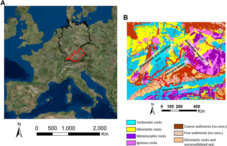
FIGURE 1. (A) Modelled area; (B) Main geological and geographical features.
Groundwater data from the Upper Danube basin, which is needed to establish the hydrogeological model, is available on the website of the Bavarian State Office for the Environment1. Data from more than 900 observational points is considered (Figure 2), but only observation points with measurements within the simulated period from 1991 to 2013, are used. Required information to implement the observation points into the model such as the locational coordinates and the depth of the screen is also obtained from the Bavarian State Office for the Environment.
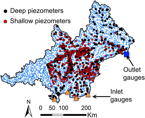
FIGURE 2. Position of available observation points at the modeled area and inlet and outlet gauging stations used for the hydrological model mHM.
2.2 Mesoscale hydrological model (mHM)
2.2.1 Code description
mHM is a spatially explicit hydrological model (Samaniego et al., 2010; Samaniego et al., 2021). It considers a wide range of surface processes such as canopy interception, snow accumulation and melting, soil moisture dynamics, infiltration and surface runoff, evapotranspiration, baseflow, discharge attenuation, and flow routing (Samaniego et al., 2010; Kumar et al., 2013). mHM has been successfully applied to several catchments across the globe and has been demonstrated to outperform many hydrological models. It has been applied to basins ranging in size from 4 to 550,000 km2 and at variable spatial resolutions (or grid size) (between 1 km and 100 km) (see www.ufz.de/mhm for more details).
2.2.2 Model set-up
In this study, mHM delivers the groundwater recharge. mHM is established following Zink et al. (2017). The simulation period is the same as the one which is used for the groundwater model (1/1/1991—31/12/2013) and daily time steps are chosen. Streamflow from four river gauging stations is implemented to define the inflow through four boundaries where the model perimeter does not agree with the basin watershed (inlet gauges in Figure 2). The quality of this model is supported by the good fitting between the modelled and the observed river flow (Figure 3A) at the outlet gauging station (outlet gauge in Figure 2). The water flow percolating below the unsaturated zone is taken as the recharge for the groundwater model (Figure 3B).
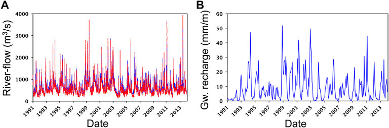
FIGURE 3. (A) Fitting between the computed (red dashed line) and the measured (blue line) river flow rate at the outlet of the basin (from 01/01/1991 to 31/12/2013); (B) Example of groundwater recharge computed with the hydrological model mHM in a cell located in the center of the modeled area (lat, lon: 73.0596, 6.70606). Recharge is shown for the period of time from 01/01/1991 to 31/12/2013.
2.3 Groundwater model
2.3.1 Code description
Groundwater flow is simulated using OpenGeoSys - OGS (Kolditz et al., 2012), an open-source scientific software platform for the numerical simulation of thermo-hydro-mechanical/chemical processes in porous media. OGS provides a flexible numerical framework (using primarily the Finite Element Method (FEM)) for solving multifield problems in porous and fractured media for applications in geoscience and hydrology. It has been recently applied in the regional groundwater modeling (Jing et al., 2018; 2019).
2.3.2 Geometrical features
The model is divided vertically into two layers whose geometry is defined using information from lithology, geology, and soil characteristics (Figure 4).
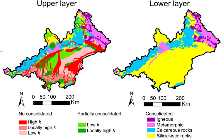
FIGURE 4. Areal distribution for parameterization considered for the two layers of the groundwater numerical model.
The hydrogeological units of the upper layer are defined by using the Hydrogeological Map of Europe (Duscher et al., 2015) and the Global Lithological Map (Hartmann and Moosdorf, 2012). These maps contain information about aquifer productivity, lithology, and degree of consolidation. The hydrogeological units of the lower layer are derived from the Geological Map of Europe (Asch, 2003). Most materials in the upper layer are unconsolidated or partially consolidated and their thickness is defined according to Shangguan et al. (2017). If the thickness (Shangguan et al., 2017) is lower than 10 m, it is assumed that the bedrock (consolidated) outcrops or reaches the top of the saturated zone. At these locations, the materials in the upper layer are also chosen according to the Geological Map of Europe, resulting in the same material for the upper and lower layer. The thickness of the formations that constitute the lower layer is not known, thus, a constant thickness of 500 m is assumed. 500 m is sufficient to minimize the impact of the lower boundary condition (no flow) in shallow water processes. The river network is implemented in the upper layer and its geometry is computed using a digital elevation model. The position and shape of major lakes and springs is obtained from the Hydrogeological Map of Europe (Duscher et al., 2015) (Figure 5).
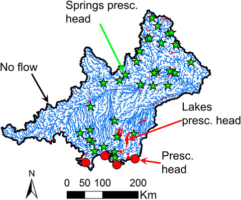
FIGURE 5. Boundary conditions of the groundwater numerical model.
2.3.3 Spatial and temporal discretization
The hydrogeological model is made up by prism elements (Sachse et al., 2015) whose average horizontal size is approximately 1,000 m and the vertical one is equal to the layer’s thicknesses. The horizontal size is not constant throughout the entire modeling domain. It is refined around wedge-shaped river intersections. Note that the geometry of the river network and the modeled formations is simplified for avoiding too small elements by reducing the number of vertexes that define the rivers. The chosen minimum distance between consecutive vertexes is 1,000 m. Steady and transient state simulations and calibrations are carried out. The transient state model simulates/calibrates from 1991 to 2013 with monthly time steps, while the steady-state model uses averaged data from the same time period.
2.3.4 Boundary conditions (BCs)
Three different types of BC are adopted. 1) No-flow BCs are implemented in the lateral boundary assuming that it agrees with the basin’s topographic watershed boundary. There are only four local exceptions in small valleys located in the Alpine region (red dots in Figure 5). In these valleys, in which the lateral boundary does not agree with the watershed, the piezometric head is prescribed according to the topography. No-flow BCs are also assumed at the bottom of the modeling domain. 2) Dirichlet BCs are implemented according to the topography to simulate the river network, the lakes, and the springs. Finally, 3) Neumann BCs are applied at the upper boundary of the model to implement a distributed groundwater recharge, which is previously computed with mHM.
2.3.5 Groundwater data
Data from piezometers located at less than 1,000 m from rivers, streams, or lakes are neglected. Otherwise, these observations would have been mapped on the same location as the prescribed head in surface water bodies due to a minimum element size of roughly 1000 m. This would have caused ambiguity and would have forced the calibration to fail. Thus, although more than 900 observation points are available, only data from 200 piezometers are used. Note that some of these 200 piezometers do not contain measurements during the simulation period or the time series is incomplete, which reduces the number of usable observations to 137.
2.3.6 Calibration software
The groundwater model is calibrated by means of the code PEST (Doherty, 1994). PEST is a non-linear parameter estimation software that can be adapted to any simulation code (i.e., it is model-independent) and uses the Gauss-Marquardt-Levenberg method that reduces the discrepancies between computed and measured data to a minimum in the weighted least squares sense (Doherty, 1994) (see the PEST Homepage2 for more details).
3 Results and discussion—Model calibration
In this section, we present the results of the model that is initially calibrated in a steady state following the standard approach, thus, by fitting heads locally to estimate K. The limitations of this standard approach are demonstrated and discussed through the calibration process. Then, a novel calibration strategy is proposed to address the main limitations of the standard one. Finally, the new approach is compared with the alternative approach of Fan et al. (2013).
3.1 Standard parametrization
Initially, the steady state model was calibrated to estimate K by fitting piezometric heads locally. However, three difficulties arose: 1) a relatively low sensitivity of the piezometric head to the K estimates, 2) the influence of the boundary conditions adopted at rivers close to observation points, and 3), problems related to the coarse horizontal and vertical discretization.
3.1.1 Low sensitivity to the K estimates
Although the measured and simulated piezometric heads fitted well under steady state conditions, similar fittings and acceptable calibration results were obtained when the values of K were modified. This fact does not reflect per se a low sensitivity of the piezometric head with respect to K, it only reveals that the variations of the computed piezometric head at the observation points when K is modified are too small to affect substantially the calibration results of a regional hydrogeological model, in which differences between computed and observed piezometric heads could be considered as acceptable. From theory we know that, the maximum elevation (with respect to the hydraulic head in the rivers) of the piezometric head (hmax [L]) occurs in the groundwater divide between two rivers (Chesnaux, 2013). The equation for calculating hmax that is derived from the general Forchheimer’s solution, is given by (Bear, 1988) as follows:
where W [L3T−1] is the groundwater recharge, X [L] is the separation between the two rivers and T [L2T−1] is the transmissivity (
To demonstrate this aspect further, the piezometric heads at the observation points computed with two scenarios with different values of K are compared. The values of K are increased and decreased by one order of magnitude with respect to those obtained from the final calibration (i.e., K values between the two compared scenarios differ by two orders of magnitude). The good fitting between the piezometric head computed at observation points for both scenarios (Figure 6), the high Pearson correlation coefficient R) (>0.99) and the low root mean square error (RMSE) (1.3 m) indicates that the steady-state piezometric head in the observation points is not enough sensitive to K. Thus, calibrated values of K with the steady state model were not reliable.
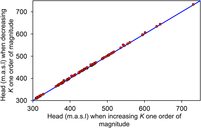
FIGURE 6. Linear regression plot between the steady state piezometric head computed with two numerical models whose values of K differ in two orders of magnitude. Piezometric head is computed at observation points used to calibrate the model. Only observation points representing piezometers screened in shallow aquifers are considered (i.e., 96 piezometers).
3.1.2 Proximity of the observation points to rivers
Although observation points located less than 1,000 m apart from rivers were neglected for the calibration, the used observation points were relatively close to rivers considering the coarse horizontal discretization of the model. For example, only one mesh node may be between a river and observation points located at 2,000 m. Thus, the computed “absolute” elevation of the piezometric head in the observation points is strongly dominated by the river hydraulic head.
3.1.3 The problem of coarse horizontal discretization
If observation points are not located at model nodes, the simulation code assigns them to the nearest node. Thus, in certain cases, observation points are assigned to far nodes when a coarse discretization is used. Near the rivers, where the smallest elements are located, the distance between the actual position of the observation points and the assigned node can reach up to 500 m. Two different situations arise in these cases. On the one hand, the computed piezometric head may differ from the real one because of the hydraulic gradient. For example, assuming a realistic hydraulic gradient in flat areas of 0.001 and a maximum displacement of 500 m, the computed piezometric head would be 0.5 m higher or lower than the measured piezometric head. Thus, there is a minimum error of ±0.5 m encountered, arising between the hydraulic gradient and the displacement of the observation points. This error increases with higher hydraulic gradients than 0.001, which commonly appear in steeper terrains, and far from rivers where the size of the elements gets larger. On the other hand, when observation points are displaced, their elevation is also modified. If an observation point is assigned to a node that is located at an elevation 100 m higher than its actual elevation, it is not possible to fit the modeled piezometric head with the observed one. This effect is most relevant in steep areas because the change in elevation within a single element is higher than in flat areas. For this reason, the error is smaller in flat areas, especially when the shallow piezometers are considered, while it can reach several meters for piezometers located at steeper terrain areas (Figure 7).
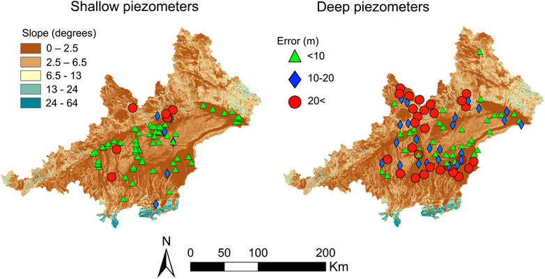
FIGURE 7. Residual error at the observation points obtained with the steady state calibration for shallow (right) and deep (left) piezometers. Results are shown on a surface slope map to show how the slope influences the residual error.
3.1.4 The problem of coarse vertical discretization
The model is vertically divided into three mesh layers, one representing the unconsolidated materials and two for the bedrock. For practical purposes, it is possible to consider that the vertical resolution does not really exist. Therefore, no vertical gradients can be resolved and observations are difficult to be addressed in a model node. This issue is reflected in the fact that errors are higher in deep piezometers than those in shallow ones (Figure 7). Given the relatively small thickness of the upper layer, shallow observation points are less vertically displaced (to be assigned to nodes) minimizing the error. As a result, the model cannot be calibrated by fitting the absolute piezometric head in a steady state. Thus, the calibration should be done under transient modeling conditions. However, the lack of accuracy in computing the exact elevation of the piezometric head also complicates the parametrization under transient conditions.
3.1.5 Consequences of the displacement of the observation points in the calibration process under transient conditions
Two different situations may arise during the calibration process due to the effects associated with the displacement of an observation point: the computed piezometric head can be located above (case 1) or below (case 2) the measured one (Figure 8). If the computed piezometric head is located above, the value of K is increased during the calibration so to decrease the objective function for fitting the average piezometric head, but, the increase of K smooths the groundwater oscillations/fluctuations that cannot be fitted. Contrary, the value of K is decreased to improve the objective function in case 2 (the computed piezometric head is located below the measured one). In this case, the average piezometric head increases but also the magnitude of the oscillations which further complicates the fitting process. In either situation, calibrated parameters by fitting the piezometric head are not representative because they do not allow reproducing correctly the groundwater oscillations. To deal with these issues, we propose an alternative calibration strategy, detailed below.
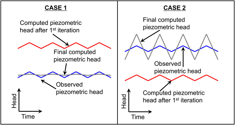
FIGURE 8. Situations that may arise when the numerical model assigns an observation point to the nearest node.
3.2 New calibration strategy
To avoid the difficulties associated to the “traditional” approach and discussed in the previous subsection, such as the low sensitivity of the piezometric head concerning K during steady state calibrations or the errors when computing the absolute elevation of the piezometric head that makes impossible the fitting, a new strategy is proposed which does not rely on the absolute values of groundwater heads but on their anomalies or relative fluctuations. The new strategy is composed of two steps. In the first step, lower and upper bounds for hydraulic parameters are identified. Within these prescribed bounds, hydraulic parameters are fitted in a second step against temporal moments of local groundwater time series.
3.2.1 Lower bounds for the hydraulic conductivity
Considering that the piezometric head increases with low values of K and that groundwater cannot be located above the surface, a steady state calibration assuming the groundwater table is located near the surface (2 m below) leads to the lower bound of K. Although its simplicity, this procedure allows establishing objectively the lower bound of K. The calibration is carried out by fitting the computed piezometric head with the surface elevation at points distributed regularly through the modeled domain. The number of points and their location is chosen arbitrarily. We consider one point every 8,000 m to undertake this calibration stage (Figure 9A). If selected points fall near rivers or streams (less than 1,000 m), they are not considered during the calibration to avoid the influence of the BCs.
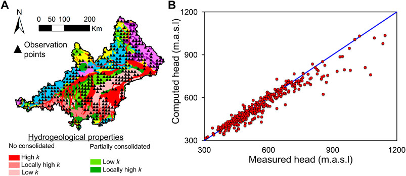
FIGURE 9. (A) Considered points to calibrate the model in steady state using the topography as reference. These points, which are chosen arbitrarily, are distributed regularly through the modeled domain. The head assigned to these points to calibrate the lower bound of the hydraulic conductivity is obtained by subtracting 2 m to the elevation surface. Despite one point every 8000 m is chosen, those located near rivers or streams are neglected; (B) Fitting between computed and measured heads derived from the topography.
The high R-value (0.987), when comparing the computed heads with those derived from topography at the selected points regularly distributed through the modeled domain, indicates that the computed piezometric head is located near the surface (Figure 9B), and thus, that the calibrated value for K can be considered as its lower bound (Table 1).
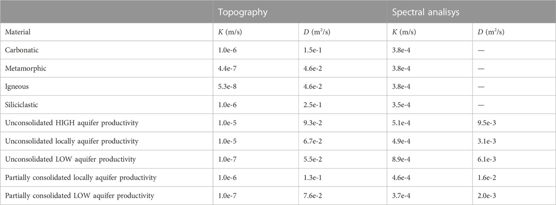
TABLE 1. Hydraulic parameters derived from the steady state calibration using as reference the topography and the spectral analyses.
3.2.2 Upper bounds for hydraulic parameters
Information concerning K and the storage coefficient (S [-]) can be also obtained by analyzing base-flow data and application of spectral analyses (Houben et al., 2022). For that purpose, the time series of river baseflow is transferred into the frequency domain for the river flow data (Gelhar, 1974) or piezometric head data (Jiménez-Martínez et al., 2013). This technique is applied to daily data ranging from 1/1/1991 to 31/12/2017 from gauging stations that are strategically chosen according to lithology/geology to obtain information about the different materials (i.e., only observation points located in sub-basins mostly containing one type of material are used) (Figure 10A). Baseflow is computed from river flow data using the digital filter method proposed by Lyne and Hollick (1979). The spectrum of the piezometric head (Shh), the recharge (SRR) and the baseflow (Sqq) are related as follows (Zhang and Schilling, 2004):
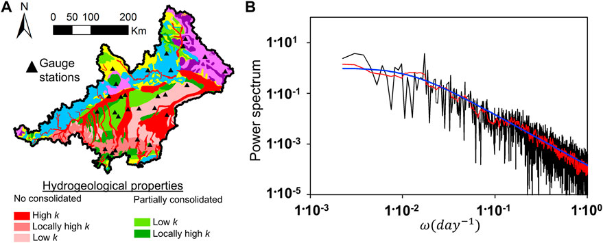
FIGURE 10. (A) Gauging stations whose data is assessed by means of the spectral analyses. These has been chosen to obtain representative results for materials with different hydrological properties. (B) Example of a the original computed power spectrum (black line) and after a filtering process (red line) for the base flow measured at one gauge (gauge number 22 in the Supplementary Material) together with the fitted curve (blue line).
and,
where ω [T−1] is the frequency, a [-] is the discharge constant or recession coefficient for a linear reservoir (
where f(ω) is the baseflow normalized function. Computed spectra are automatically fitted to Eq. (4) by using PEST (Figure 10B). Then, the hydraulic diffusivity (
where D is the drainage density [L−1] (Horton, 1932).
Information concerning S is needed to calculate the T from
The power spectrum of the selected gauging stations is smoothed by applying a filtering tool to facilitate the fitting (Figure 10B). The power spectra of all considered gauging stations are shown in the Supplementary Material.
Baseflow is an integrative water flux provided by the different geologic formations in the basin, and the flow toward rivers is primarily along high conductivity flow paths. Consequently, values of T (and K) derived from spectral analyses of the baseflow are biased towards higher transmissivity values. Consequently, the results from spectral analyses are assumed to be upper bounds of K (Table 1). In the same manner, the value of S derived from spectral analysis (Table 1) is used to constrain the upper bound of SS (Jiménez-Martínez et al., 2013). In our case, (6·10−3 m−1) is used as the upper bound. Information about the lower bound is not available. Thus, values of 10−4 m−1 and 10−5 m−1 are assumed for the unconsolidated and consolidated materials. A lower value is used for the consolidated materials since they are mainly from confined aquifers in the bedrock.
3.2.3 Local model calibration based on statistical moments
Four alternative calibration techniques are conducted to circumvent the complications emerging from the standard parametrization approach. The first method (M1) consists in fitting the piezometric head anomalies without considering the absolute position of the piezometric head. The difference between the computed and observed piezometric heads is corrected after each iteration taking as reference the initial head difference between them. In this way, difficulties associated with the computation of the absolute position of the piezometric head are avoided. The other three methods are based on fitting statistical parameters of the piezometric head time series. In method 2 (M2) the model is calibrated by fitting the variance of the measured against computed piezometric heads. The third method (M3) matches the Pearson correlation coefficient R of the computed and measured piezometric head at each observation point. Finally, in the fourth method (M4), the model is jointly calibrated using the variance and the Pearson correlation coefficient R.
The fitting between measured and computed piezometric heads with the four calibration methods gave acceptable results at all locations of the modeled basin (Figure 11). Given the number of piezometers used for the calibration, R and RMSE (root mean square error) values are used to evaluate its quality. R and RMSE values are computed for all the observation points (Table 2). They are also calculated with and without applying a bias, accounting for the change in the elevation of the piezometers induced by the numerical model. R and RMSE are firstly calculated considering every observation point without applying a bias correction. In this case, R and RMSE are around 0.95 and 19 m for all calibration methods. Both values are acceptable considering the coarse resolution, the range of simulated piezometric heads (from 309 to 733 m. a.s.l), and especially, the spatial discretization of the model. R and RMSE values are improved substantially when the shift in the elevation of the observation points is eliminated. In this case, R values are higher than 0.99 while RMSE values range between 1.13 and 1.14 m. The indicators (R and RMSE) are so similar among different methods such that it is not possible to discern the best calibration method.
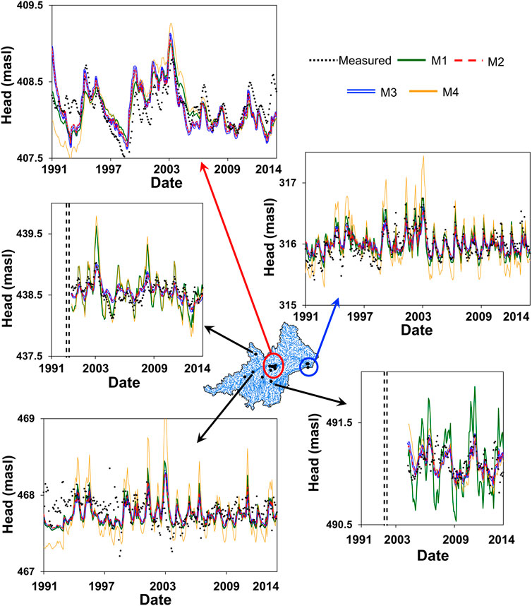
FIGURE 11. Fitting between measured and computed piezometric heads at 5 observation points. Results considering the four calibration methods (M1-M4) are included.
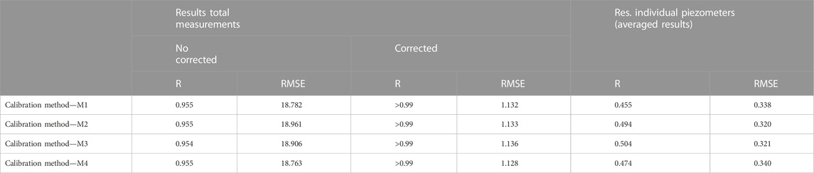
TABLE 2. Statistical results of the transient calibrations.
R and RMSE are also calculated individually for each piezometer (Table 2). Slight differences can be observed when comparing the distribution of individual R obtained with each one of the calibration methods (Figure 12). Values of individual R range between 0.45 for the calibration method M1 to 0.5 for the calibration method M3. The highest R values are obtained for the calibration methods M2 and M3. RMSE values oscillate between 0.34 (M1) to 0.32 (M2), which are acceptable considering the average individual variance. The individual analysis of the observation points provides relevant information concerning the best calibration method. Although differences are not too large, the best values of R and RMSE are obtained with the calibration method M2 (i.e., using the variance as reference).
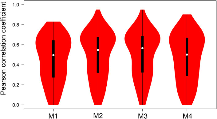
FIGURE 12. Individual R distribution obtained with each calibration method. White circles show the medians; box limits indicate the 25th and 75th percentiles as determined by R software; whiskers extend 1.5 times the interquartile range from the 25th and 75th percentiles; polygons represent density estimates of data and extend to extreme values.
The computed parameters for each one of the calibrations (Table 3) are similar for most of the hydrological units and agree with the materials. There are only some exceptions in which the calibrated value varies among calibrations. Probably, it occurs because, exceptionally, the fitted variable (or variables), which varies for each calibration method, is not sensitive to the calibrated parameter. Even though several challenges arose from the large domain size and coarse discretization, different calibration methods led to very similar and reasonable estimates of hydraulic parameters with small errors. Although results are similar for all the calibration methods, it is important to highlight that, in our case, due to the “master-slave” paradigm used by the parallel PEST (Doherty, 2010; Wang et al., 2019), the computation time decreases when statistical parameters are used because input files are much lighter than that used when all the piezometric head observations are considered.
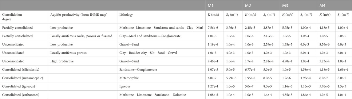
TABLE 3. Calibrated hydraulic parameters with the transient model.
The steady state results are computed and compared with the measured ones by using the calibrated parameters with the method M2 (Figure 13A). R and RMSE values are >0.98 and 9.9 m, respectively, when only the shallow piezometers are regarded, while R and RMSE are 0.93 and 23 m, respectively, when all the piezometers are considered. The piezometric head distribution considering the parameters derived with method M2 is realistic and, as expected, is controlled by the topography (Figure 13B).
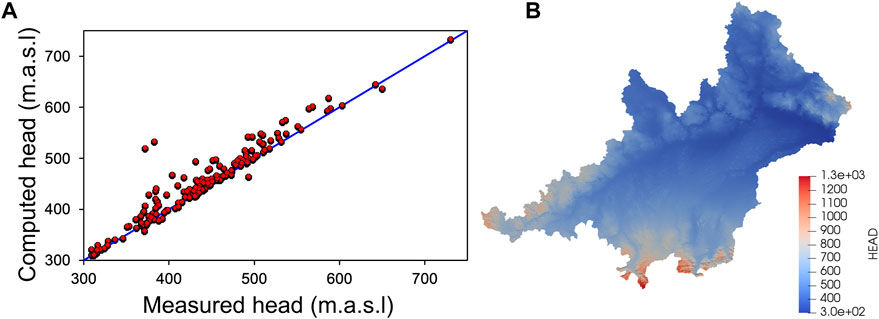
FIGURE 13. (A) Fitting between measured and computed steady state piezometric heads. The simulation is undertaken using the K values calibrated with the method M2. In M2 the model is calibrated by fitting the variance of the measured and computed piezometric heads; (B) Steady state piezometric head distribution when K values obtained with method M2 are used.
3.3 Comparison with previous approaches
The proposed new approach (NA) is compared with that used in previous studies (PA) by other authors (Fan et al., 2013; de Graaf et al., 2015). To do so, we establish a groundwater model analogous to (Fan et al., 2013). The characteristics of the groundwater model are parametrized according to the following procedure It consists of a 2D model in which the horizontal discretization and BCs are the same as those adopted for developing the model with the NA approach. The thickness is computed using the e-folding depth method as
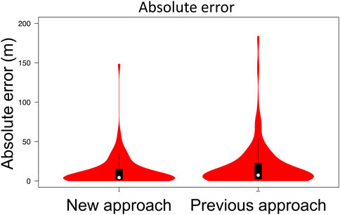
FIGURE 14. Absolute error between measurements and computed piezometric heads in steady state with the NA and PA approaches. White circles show the medians, box limits indicate the 25th and 75th percentiles as determined by R software, whiskers extend 1.5 times the interquartile range from the 25th and 75th percentiles and polygons represent density estimates of data and extend to extreme values.
Although results from the new (NA) approach are slightly better, the computed piezometric heads are similar in both approaches at observation point located in valleys. However, large differences can be observed when comparing the water table depth (Figure 15) in mountainous areas where the water table computed using the PA approach is above the terrain surface. In other words, the groundwater model developed using the PA approach fails to compute the piezometric head in these areas. This fact is probably related to a too low computed thickness by means of the e-folding depth method.
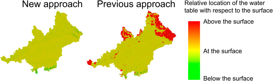
FIGURE 15. Relative location of the water table depth. Green means that the water table depth is below the surface, yellow that the water table is close to the surface (some meters below or above), while red indicates areas where the water table is much higher than the surface.
4 Conclusion
Our work assesses difficulties that arise when developing large-scale groundwater models and proposes an approach to tackle the model parameterization problem. In fact, it addresses the main challenges of global groundwater models development stated by other authors such as Reinecke et al. (2019) who highlight that the main difficulties of global models are related to the lack of data to define the parameters and the geometry of the hydrogeological systems and the needed large spatial resolutions. The proposed methodology in this work allows the development of a large-scale numerical model, adopting similar limitations to other existing models, capable to reproduce the general groundwater behaviour. This means that the same (or a similar) methodology could be used to model larger areas than in this study.
Through this work, we have verified that, among others, one of the main difficulties when developing large-scale groundwater models is the lack of suitable information to define the hydraulic parameters, the behaviour and the geometry of hydrogeological units. Although, there are some globally available datasets, they often lack relevant information to parametrise and develop reliable groundwater models.
Furthermore, complications related to the spatial discretization and the boundary conditions are often encountered during the calibration process. Although these difficulties could be minimized by reducing the size of the elements in the model domain, it would require enormous computational power to model larger areas. Therefore, four alternative methods are used to calibrate the model in transient state, three of which are based on statistical parameters (variance and R) derived from the piezometric head evolution. The obtained results with the four calibration methods are acceptable and very similar. The results from the variance-based calibration, i.e., calibration of the model by fitting the variance of the measured and computed piezometric heads, are slightly better than those obtained with the other methods. A relevant fact, especially for the calibration of large models with parallel PEST, is that calibrations based on statistic values derived from piezometric heads require less computation time due to the low weight of input files in comparison with those used when all piezometric observations are considered.
The results also show that continental/global scale groundwater models are really complicated to be calibrated in steady state because the piezometric head in high transmissive areas is only little sensitive to the hydraulic parameters, and variations due to different values of K are lower than the error in the piezometric head elevation induced by the coarse discretization. This issue is relevant because many of the large-scale groundwater models developed up to date are only calibrated in steady state.
Piezometric head data may not be available to calibrate the hydraulic parameters of large areas. In these situations, the methodology used to constrain the upper and lower bounds of hydraulic parameters could be applied to improve the calibration performance and reduce their uncertainty. Later, the groundwater behavior could be computed by considering these estimated bounds. If required river data to compute the spectral analyses of the baseflow is not available, streamflow simulations from calibrated hydrologic models, such as mHM (Samaniego et al., 2010) could be used.
It is expected that the proposed calibration strategy works also properly when using a coarse mesh like that used in previous global models, such as that of de Graaf et al. (2015). Theoretically, the error in computing the absolute elevation of the piezometric head could increase with spatial discretization. However, this does not affect the quality of the proposed calibration strategy since it consists of fitting statistical moments or piezometric head anomalies. In addition, the proposed approach to define the minimum and maximum boundaries of K and S can be used in the same manner. Overall, the proposed calibration approach allows for obtaining better results than adopting previous methodologies used for developing regional or global models, especially in mountainous areas where previous approaches tend to underestimate the saturated thickness, and therefore, to overestimate the piezometric head.
Data availability statement
The original contributions presented in the study are included in the article/Supplementary Material, further inquiries can be directed to the corresponding authors.
Author contributions
EP: Conceptualization, investigation, methodology, visualization, writing—Original draft. RK: Resources, methodology, writing-reviewing. TH: Methodology, software, visualization, writing-reviewing. MJ: Software, writing- reviewing. OR: Resources, writing-reviewing. TK: Methodology, software, writing-reviewing. SA: Conceptualization, funding acquisition, investigation, methodology, supervision, writing- reviewing.
Funding
This research has been supported within the research initiative “Global Resource Water (GRoW; 02WGR1423A-F)”. GRoW is part of the Sustainable Water Management (NaWaM) funding priority within the Research for Sustainable Development (FONA) framework of the German Federal Ministry of Education and Research (BMBF). EP gratefully acknowledges the support received through the grant CEX2018-000794-S funded by MCIN/AEI/10.13039/501100011033, the grant RYC2020-029225-I funded by MCIN/AEI/10.13039/501100011033 and by “ESF Investing in your future” and the Award for Scientific Research into Urban Challenges in the City of Barcelona 2020 (20S08708) from the Barcelona city council.
Conflict of interest
The authors declare that the research was conducted in the absence of any commercial or financial relationships that could be construed as a potential conflict of interest.
Publisher’s note
All claims expressed in this article are solely those of the authors and do not necessarily represent those of their affiliated organizations, or those of the publisher, the editors and the reviewers. Any product that may be evaluated in this article, or claim that may be made by its manufacturer, is not guaranteed or endorsed by the publisher.
Supplementary material
The Supplementary Material for this article can be found online at: https://www.frontiersin.org/articles/10.3389/feart.2023.1061420/full#supplementary-material
Footnotes
1https://www.gkd.bayern.de/en/[Accessed 8 December 2022]
2https://pesthomepage.org/[Accessed 7 December 2022]
References
Asch, K. (2003). The 1:5 million international geological map of Europe and - adjacent areas. Available at: https://www.schweizerbart.de/publications/detail/artno/188010003 (Accessed May 7, 2021).
A. Baba, G. Tayfur, O. Gündüz, K. W. F. Howard, M. J. Friedel, and A. Chambel (Editors) (2011). Climate change and its effects on water resources: Issues of national and global security (Netherlands: Springer). doi:10.1007/978-94-007-1143-3
Barthel, R., Rojanschi, V., Wolf, J., and Braun, J. (2005). Large-scale water resources management within the framework of GLOWA-Danube. Part A: The groundwater model. Phys. Chem. Earth, Parts A/B/C 30, 372–382. doi:10.1016/j.pce.2005.06.003
Camporese, M., Paniconi, C., Putti, M., and Orlandini, S. (2010). Surface-subsurface flow modeling with path-based runoff routing, boundary condition-based coupling, and assimilation of multisource observation data. Water Resour. Res. 46. doi:10.1029/2008WR007536
Chesnaux, R. (2013). Regional recharge assessment in the crystalline bedrock aquifer of the Kenogami Uplands, Canada. Hydrological Sci. J. 58, 421–436. doi:10.1080/02626667.2012.754100
de Graaf, I. E. M., Sutanudjaja, E. H., van Beek, L. P. H., and Bierkens, M. F. P. (2015). A high-resolution global-scale groundwater model. Hydrol. Earth Syst. Sci. 19, 823–837. doi:10.5194/hess-19-823-2015
de Graaf, I. E. M., van Beek, R. L. P. H., Gleeson, T., Moosdorf, N., Schmitz, O., Sutanudjaja, E. H., et al. (2016). A global-scale two-layer transient groundwater model: Development and application to groundwater depletion. Hydrology Earth Syst. Sci. Discuss. 11, 1–30. doi:10.5194/hess-2016-121
Dingman, S. L. (1978). Drainage density and streamflow: A closer look. Water Resour. Res. 14, 1183–1187. doi:10.1029/WR014i006p01183
Doherty, J. (1994). Pest: A unique computer program for model-independent parameter optimisation. Water Down Under 94 Groundwater/Surface Hydrology Common Interest Pap. Prepr. Pap. 11, 551–554. doi:10.3316/informit.752715546665009
Duscher, K., Günther, A., Richts, A., Clos, P., Philipp, U., and Struckmeier, W. (2015). The GIS layers of the "international hydrogeological map of Europe 1:1,500,000" in a vector format. Hydrogeol. J. 23, 1867–1875. doi:10.1007/s10040-015-1296-4
Fan, Y., Li, H., and Miguez-Macho, G. (2013). Global patterns of groundwater table depth. Science 339, 940–943. doi:10.1126/science.1229881
Gardner, M. A., Morton, C. G., Huntington, J. L., Niswonger, R. G., and Henson, W. R. (2018). Input data processing tools for the integrated hydrologic model GSFLOW. Environ. Model. Softw. 109, 41–53. doi:10.1016/j.envsoft.2018.07.020
Gelhar, L. W. (1974). Stochastic analysis of phreatic aquifers. Water Resour. Res. 10, 539–545. doi:10.1029/WR010i003p00539
Gleeson, T., Moosdorf, N., Hartmann, J., and van Beek, L. P. H. van (2014). A glimpse beneath Earth's surface: GLobal HYdrogeology MaPS (GLHYMPS) of permeability and porosity. Geophys. Res. Lett. 41, 3891–3898. doi:10.1002/2014GL059856
Gleeson, T., Smith, L., Moosdorf, N., Hartmann, J., Dürr, H. H., Manning, A. H., et al. (2011). Mapping permeability over the surface of the Earth. Geophys. Res. Lett. 38, a–n. doi:10.1029/2010GL045565
Hartmann, J., and Moosdorf, N. (2012). The new global lithological map database GLiM: A representation of rock properties at the earth surface. Geochem. Geophys. Geosyst. 13. doi:10.1029/2012GC004370
Hellwig, J., Graaf, I. E. M., Weiler, M., and Stahl, K. (2020). Large-scale assessment of delayed groundwater responses to drought. Water Resour. Res. 56–e2019WR025441. doi:10.1029/2019WR025441
Hoekstra, A. Y., and Mekonnen, M. M. (2012). The water footprint of humanity. Proc. Natl. Acad. Sci. U.S.A. 109, 3232–3237. doi:10.1073/pnas.1109936109
Horton, R. E. (1932). Drainage-basin characteristics. Trans. AGU 13, 350–361. doi:10.1029/TR013i001p00350
Houben, T., Pujades, E., Kalbacher, T., Dietrich, P., and Attinger, S. (2022). From dynamic groundwater level measurements to regional aquifer parameters–assessing the power of spectral analysis. Water Resources Research, e2021WR031289. doi:10.1029/2021WR031289
Ivanov, V. Y., Vivoni, E. R., Bras, R. L., and Entekhabi, D. (2004). Catchment hydrologic response with a fully distributed triangulated irregular network model. Water Resour. Res. 40. doi:10.1029/2004WR003218
Jiménez-Martínez, J., Longuevergne, L., Le Borgne, T. L., Davy, P., Russian, A., and Bour, O. (2013). Temporal and spatial scaling of hydraulic response to recharge in fractured aquifers: Insights from a frequency domain analysis. Water Resour. Res. 49, 3007–3023. doi:10.1002/wrcr.20260
Jing, M., Heße, F., Kumar, R., Kolditz, O., Kalbacher, T., and Attinger, S. (2019). Influence of input and parameter uncertainty on the prediction of catchment-scale groundwater travel time distributions. Hydrol. Earth Syst. Sci. 23, 171–190. doi:10.5194/hess-23-171-2019
Jing, M., Heße, F., Kumar, R., Wang, W., Fischer, T., Walther, M., et al. (2018). Improved regional-scale groundwater representation by the coupling of the mesoscale Hydrologic Model (mHM v5.7) to the groundwater model OpenGeoSys (OGS). Geosci. Model Dev. 11, 1989–2007. doi:10.5194/gmd-11-1989-2018
Kolditz, O., Bauer, S., Bilke, L., Böttcher, N., Delfs, J. O., Fischer, T., et al. (2012). OpenGeoSys: An open-source initiative for numerical simulation of thermo-hydro-mechanical/chemical (THM/C) processes in porous media. Environ. Earth Sci. 67, 589–599. doi:10.1007/s12665-012-1546-x
Kumar, M., Duffy, C. J., and Salvage, K. M. (2009). A second-order accurate, finite volume-based, integrated hydrologic modeling (FIHM) framework for simulation of surface and subsurface flow. Vadose Zone J. 8, 873–890. doi:10.2136/vzj2009.0014
Kumar, R., Samaniego, L., and Attinger, S. (2013). Implications of distributed hydrologic model parameterization on water fluxes at multiple scales and locations. Water Resour. Res. 49, 360–379. doi:10.1029/2012WR012195
Marke, T. (2008). Development and application of a model interface to couple land surface models with regional climate models for climate change risk assessment in the upper Danube watershed. Available at: https://edoc.ub.uni-muenchen.de/9162/(Accessed May 6, 2022).
Markstrom, S., Niswonger, R., Regan, R., Prudic, D., and Barlow, P. (2008). GSFLOW—coupled ground-water and surface-water flow model based on the integration of the precipitation-runoff modeling system (PRMS) and the modular ground-water flow model. MODFLOW-2005) 10. doi:10.13140/2.1.2741.9202
Mauser, W., and Prasch, M. (2015). Regional assessment of global change impacts - the project GLOWA-danube.China
Maxwell, R. M., Condon, L. E., and Kollet, S. J. (2015). A high-resolution simulation of groundwater and surface water over most of the continental US with the integrated hydrologic model ParFlow v3. Geosci. Model Dev. 8, 923–937. doi:10.5194/gmd-8-923-2015
Maxwell, R. M., and Miller, N. L. (2005). Development of a coupled land surface and groundwater model. J. Hydrometeorol. 6, 233–247. doi:10.1175/JHM422.1
McDonald, M. G., and Harbaugh, A. W. (1984). A modular three-dimensional finite-difference ground-water flow model. U.S. Geol. Surv. 23. doi:10.3133/ofr83875
Pelletier, J. D., Broxton, P. D., Hazenberg, P., Zeng, X., Troch, P. A., Niu, G.-Y., et al. (2016). A gridded global data set of soil, intact regolith, and sedimentary deposit thicknesses for regional and global land surface modeling. J. Adv. Model Earth Syst. 8, 41–65. doi:10.1002/2015MS000526
Qu, Y., and Duffy, C. J. (2007). A semidiscrete finite volume formulation for multiprocess watershed simulation. Water Resour. Res. 43. doi:10.1029/2006WR005752
Reinecke, R., Foglia, L., Mehl, S., Trautmann, T., Cáceres, D., and Döll, P. (2019). Challenges in developing a global gradient-based groundwater model (G<sup>3</sup>M v1.0) for the integration into a global hydrological model. Geosci. Model Dev. 12, 2401–2418. doi:10.5194/gmd-12-2401-2019
Sachse, A., Rink, K., He, W., and Kolditz, O. (2015). OpenGeoSys-tutorial: Computational hydrology I: Groundwater flow modeling. Springer. Midtown Manhattan, NY
Samaniego, L., Thober, S., Kumar, R., Wanders, N., Rakovec, O., Pan, M., et al. (2018). Anthropogenic warming exacerbates European soil moisture droughts. Nat. Clim. Change 8, 421–426. doi:10.1038/s41558-018-0138-5
Samaniego, L., Kumar, R., and Attinger, S. (2010). Multiscale parameter regionalization of a grid-based hydrologic model at the mesoscale. Water Resour. Res. 46. doi:10.1029/2008WR007327
Shangguan, W., Hengl, T., Mendes de Jesus, J. M. de, Yuan, H., and Dai, Y. (2017). Mapping the global depth to bedrock for land surface modeling. J. Adv. Model. Earth Syst. 9, 65–88. doi:10.1002/2016MS000686
Shen, Y., and Chen, Y. (2009). Global perspective on hydrology, water balance, and water resources management in arid basins. Hydrol. Process. 24, a–n. doi:10.1002/hyp.7428
Shiklomanov, I. (1993). “World fresh water resources,” in Water in crisis: A guide to the world’s (Oxford New York: Oxford University Press, IncOxford University Press).
Sowers, J., Vengosh, A., and Weinthal, E. (2011). Climate change, water resources, and the politics of adaptation in the Middle East and North Africa. Clim. Change 104, 599–627. doi:10.1007/s10584-010-9835-4
Srivastava, V., Graham, W., Muñoz-Carpena, R., and Maxwell, R. M. (2014). Insights on geologic and vegetative controls over hydrologic behavior of a large complex basin - global Sensitivity Analysis of an integrated parallel hydrologic model. J. Hydrology 519, 2238–2257. doi:10.1016/j.jhydrol.2014.10.020
Sutanudjaja, E. H., van Beek, L. P. H., de Jong, S. M., van Geer, F. C., and Bierkens, M. F. P. (2011). Large-scale groundwater modeling using global datasets: A test case for the rhine-meuse basin. Hydrol. Earth Syst. Sci. 15, 2913–2935. doi:10.5194/hess-15-2913-2011
Therrien, R., McLaren, R. G., Sudicky, E. A., and Panday, S. M. (2004). HydroSphere: A three-dimensional numerical model describing fully-integrated subsurface and surface flow and solute transport. Waterloo, ON: University of Waterloo.
Wang, J., Wang, C., Rao, V., Orr, A., Yan, E., and Kotamarthi, R. (2019). A parallel workflow implementation for PEST version 13.6 in high-performance computing for WRF-hydro version 5.0: A case study over the midwestern United States. Geosci. Model Dev. 12, 3523–3539. doi:10.5194/gmd-12-3523-2019
Zhang, Y.-K., and Schilling, K. (2004). Temporal scaling of hydraulic head and river base flow and its implication for groundwater recharge. Water Resour. Res. 40. doi:10.1029/2003WR002094
Zink, M., Kumar, R., Cuntz, M., and Samaniego, L. (2017). A high-resolution dataset of water fluxes and states for Germany accounting for parametric uncertainty. Hydrology and Earth System Sciences 21 (3), 1769–1790.
Keywords: regional numerical modeling, hydrological modelling, mHM model, OpenGeoSys, groundwater modelling, spectral analysis
Citation: Pujades E, Kumar R, Houben T, Jing M, Rakovec O, Kalbacher T and Attinger S (2023) Towards the construction of representative regional hydro(geo)logical numerical models: Modelling the upper Danube basin as a starting point. Front. Earth Sci. 11:1061420. doi: 10.3389/feart.2023.1061420
Received: 04 October 2022; Accepted: 09 January 2023;
Published: 27 January 2023.
Edited by:
Francesca Pianosi, University of Bristol, United KingdomReviewed by:
Carlos Duque, University of Granada, SpainMostaquimur Rahman, University of Bristol, United Kingdom
Copyright © 2023 Pujades, Kumar, Houben, Jing, Rakovec, Kalbacher and Attinger. This is an open-access article distributed under the terms of the Creative Commons Attribution License (CC BY). The use, distribution or reproduction in other forums is permitted, provided the original author(s) and the copyright owner(s) are credited and that the original publication in this journal is cited, in accordance with accepted academic practice. No use, distribution or reproduction is permitted which does not comply with these terms.
*Correspondence: Sabine Attinger, c2FiaW5lLmF0dGluZ2VyQHVmei5kZQ==; Estanislao Pujades, ZXN0YW5pc2xhby5wdWphZGVzQGlkYWVhLmNzaWMuZXM=
†Present address: Estanislao Pujades, Department of Geosciences, Institute of Environmental Assessment and Water Research (IDAEA), Severo Ochoa Excellence Center of the Spanish Council for Scientific Research (CSIC), Barcelona, Spain