 Doyoon Lim
 Jae-Kwang Ahn
- 1Earthquake and Volcano Research Division, Korea Meteorological Administration, Seoul, Republic of Korea
- 2Earthquake and Volcano Technology Team, Korea Meteorological Administration, Seoul, Republic of Korea
Earthquake detection can be improved by ensuring that seismometer sites experience little artificial noise in the surrounding environment. To minimize noise, seismological stations should be positioned in rocky mountainous areas without nearby valleys, away from significant human activity. However, such surface sites may be scarce when constructing dense monitoring networks, necessitating the use of underground sites to ensure low noise levels. The Korean Meteorological Administration is currently installing new underground seismometers to increase seismic monitoring capacity. However, seismic data on the ground surface are also required for engineering technological developments (to reduce damage to structural components). Therefore, borehole seismic stations without surface seismometers need to estimate ground surface motion from borehole record data. We propose a transfer function that converts motion within boreholes to surface seismic waves using ambient noise, thereby facilitating estimation of ground surface motions using borehole seismometers. As a result, predicting ground surface motion from borehole record data becomes possible.
1 Introduction
The Korea Meteorological Administration (KMA) detects earthquakes and analyzes the source information using its seismic monitoring network. The Korean seismic monitoring network began with two stations in 1978, which underwent rapid modernization in the 1990s (KMA, 2001; Park et al., 2011; Cho et al., 2022). The number of stations further increased following the 2016 Gyeongju earthquake (Cho et al., 2022). Currently, 282 seismometers are installed, with borehole-type seismometers being applied to new or renovated stations since 2016. Recently, seismometers, have been installed in subsurface bedrock layers, to reduce the influence of day-to-day noise. Due to their low ambient noise, these borehole stations can facilitate outstanding detection of micro earthquakes and the first signs of P-waves. As of May 2022, borehole and surface seismometers account for 85% and 15%, respectively, of seismic observation stations.
With regard to earthquake early warning (EEW) systems, installation of borehole stations is highly efficient (Cho et al., 2022; Jang et al., 2023). However, as we aimed to assess earthquake-induced damage from ground motion, we cannot neglect the management of recordings on the ground surface. Unfortunately, high installation costs and budgetary limitations have restricted the establishment of both surface and borehole observatories. As a result, there are only limited studies of how vibrations are transferred from boreholes to the ground surface in the context of the topography of the Korean Peninsula.
To solve this problem, a few studies have applied a site amplitude coefficient (SAC) (Borcherdt, 1994; BSSC, 1997; Dobry et al., 2000) that has been used in the western regions of the United States. However, this method may not be appropriate, because the geological and topographical characteristics of Korea and the United States differ, and therefore a detailed review is needed to apply this method to the Korean Peninsula (Manandhar et al., 2018). In addition, estimation techniques related to earthquake damage are based on an empirical formula that utilizes the amplitude of ground surface vibrations; thus, it is crucial to determine surface vibrations (McCann et al., 1980; Shinozuka et al., 2000; Padgett and DesRoches, 2008). To this end, it would be highly effective to install surface sensors in the borehole stations; however, this was not possible because of the available budget in Korea. Thus, it is necessary to develop a technique to estimate ground surface vibrations using subsurface sensors in order to determine ground surface behavior.
Two approaches can be used to estimate ground surface vibrations. First, in the SAC method, which was first introduced in seismic design, the underlying hard bedrock conditions are assumed to match those of rock outcrops. Based on this, an increment–decrement coefficient is applied according to the average shear-wave velocity up to 30 m from the target ground. The modified Mercalli intensity (MMI) system of the KMA uses the SAC of the Borcherdt model (Borcherdt, 1994). However, the site coefficient is not suitable as a ground surface prediction model for borehole stations, as the within-motion in the rock around the borehole differs from the rock outcrop motion in the free field (Kwak et al., 2022; Lai et al., 2022). Second, the ground response can be interpreted via numerical analysis. This approach requires characterization of materials comprising the thin soil layer. This can be achieved through ground surveys such as suspension PS (S-PS) logging, downhole testing, multichannel analysis of surface waves (MASW), and standard penetration tests. This ground surface analysis method has been shown to be highly effective in predicting ground surface vibrations (Park and Hashash, 2004). Kwak et al. (2022) proposed estimation of the ground surface response by combining the ground motion model (GMM) and 1D site response. However, this required a prior site characterize. It can be prohibitively expensive to perform such surveys at a large number of stations; moreover, at some sites, it is not feasible to conduct surveys at all.
Therefore, a new estimation method without site characterization is required to predict ground surface vibrations at borehole stations. We tried to use ambient noise for the non-experimental approaches. At this time, an ambient noise signal is utilized because it includes a resonance effect on the media. Many studies have already analyzed the correlation with the predominant and/or fundamental frequency of the site characterization from ambient noise (Albarello and Lunedei, 2010; García-Fernández and Jiménez, 2012; Cultrera et al., 2014; Moisidi et al., 2015; Asten and Hayashi, 2018). The aim of this study was to determine a transfer function to convert motion recorded at a borehole to that occurring at the ground surface, without the need for site-specific response analysis. To this end, we collected ambient noise data while operating temporary seismometers.
2 Data recorded at temporary observatories
2.1 Current status of the KMA observation network
Three types of seismometers have been installed at ∼14 km intervals in the KMA seismic station. These three types, termed surface, borehole A, and borehole B, have been installed at 41, 156, and 85 sites, respectively. Figure 1 shows the distribution of these three seismometer types across the KMA seismic monitoring network. The surface stations are mostly located in areas that are presumed to have a bedrock layer, with borehole stations installed 20 and 100 m below the ground surface. Accelerometers were also installed at 20 m and 100 m below the ground surface. For type-A boreholes, seismometers were only installed 20 m below the ground surface, whereas for type-B boreholes they were installed at both 20 and 100 m below the ground surface. Each type can be easily discerned from the code name of each station, which consists of four letters, with the first three indicating the name of the region and the last indicating the sensor type (A or B).
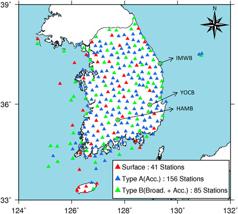
FIGURE 1. National seismic monitoring network on Korean Peninsula installed by KMA. The triangular marks indicate the Surface (red), Type-A (blue: accelerometer at 20 m depth), and Type-B (green: accelerometer at 20 m and broadband at 100 m depths) stations.
During the period over which the seismic monitoring network has been managed by the KMA, seismometers occasionally malfunctioned. A temporary seismometer (velocimeters or accelerometers) was installed on the ground surface while the malfunctioning sensor was being repaired. Therefore, seismic waves could be recorded at the ground surface and depths of 20 m during the repair period. In this study, those stations at which earthquake data were recorded by temporary seismometers.
Table 1 summarizes the selected stations and the earthquake data recorded during the times at which temporary seismometers were installed. These stations are shown in Figure 1. These data were collected based on local magnitudes (ML) ≥ 2.5 and epicenter distances <150 km. The YOCB station is close to these two locations and recorded the highest number of events during the period of temporary seismometer operation (n = 31). The IMWB and HAMB stations recorded fewer events during this period (n = 10 and n = 16, respectively).
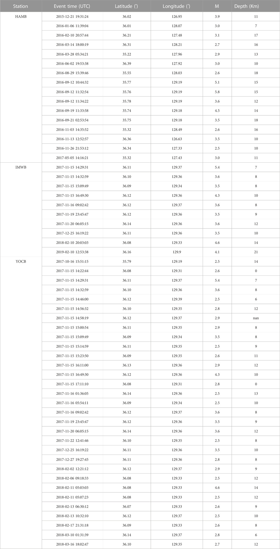
TABLE 1. Event Information during operation of temporary seismometers.
2.2 Analysis of event data at the temporary station
Figure 2 shows the accelerograms for the horizontal component borehole and surface at the three aforementioned stations. Figures 2A, B displays the seismic record from the HAMB station, showing an ML 5.8 earthquake that occurred at 11:32:54 on 09/12/2016 (UTC), 131 km from the station. Figures 2C–F show seismic recordings from IMWB and YOCB stations, respectively, for an ML 5.4 earthquake that occurred at 05:29:31 on 15/11/2017, at distances of 125 and 40 km, respectively, from the earthquake epicenter.
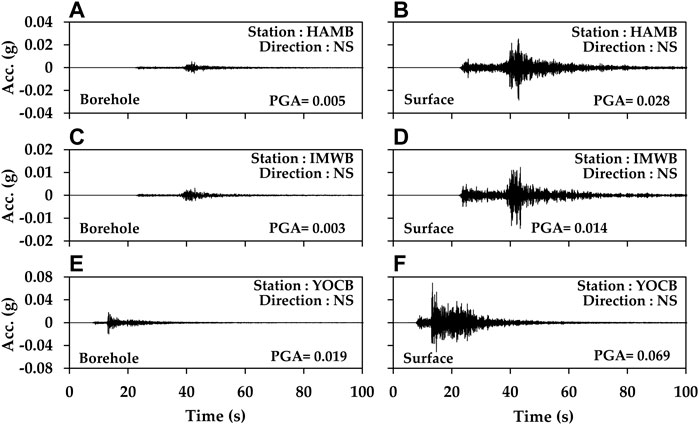
FIGURE 2. Seismic data for MKMA 5.8 earthquake occurring at 11:32:54 on 09/12/2016, recorded at HAMB station; and for MKMA 5.4 earthquake occurring at 05:29:31 on 15/11/2017 at IMWB station and YOCB station. (A,C,E) borehole and (B,D,F) surface records for NS channel of each station, respectively.
When seismic wave monitoring records are available for both borehole and surface stations, the amplification of the soil layer can be easily identified. The amplification can be calculated as the ratio of the peak ground acceleration (PGA) in both positions:
where PGAs and PGAwr are the maximum horizontal accelerations recorded at the surface ground (depth = 0 m) and boreholes (depth = 20 m), respectively. The YOCB station had the lowest peak ground acceleration (PGA) ratio between the rock outcrop and subsurface recordings at 3.85. Table 2 summarizes the average PGA ratios of surface-to-within motions for the earthquakes. In terms of average PGA ratios throughout the overall event case, the YOCB site shows a small value of 4.10, as expected. However, this value is still higher than the maximum SAC used in the Republic of Korea (MOLIT, 2018; Cho et al., 2022). The disparity in the recorded data for both indicates that the amplification table for seismic design (which is based on rock outcrop measurements) is unsuitable for estimating horizontal seismic waves at ground surface vibrations using borehole stations. This is based on the theory of wave propagation, as shown in Figure 3. Figure 3 shows that the measurement of the borehole sensor affects both the incidence wave in rock and the transit wave of soil layers over rock. Therefore, the application of the SAC method in borehole stations is barely suitable due to the differences between the borehole and rock outcrop sensors.
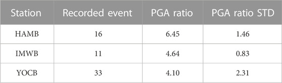
TABLE 2. PGA ratio of surface-to-within motion.
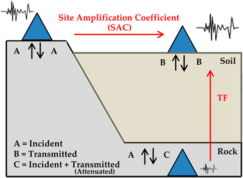
FIGURE 3. Schematic of difference between transfer function (TF) and site amplification coefficient (SAC).
If records from both the ground surface and within a rock were available, the site effect in the frequency domain from an earthquake could be calculated. The site effect indicated the amplification ratio of both the ground surface and within a rock. We called it the transfer function (TF), which is calculated as follows:
where H(ω) is the TF. Amps(ω) and Ampwr (ω) are the amplification in the frequency domain at the surface ground (depth = 0 m) and boreholes (depth = 20 m), respectively. Figure 4 illustrates the average TF of the layer, from the depth of the borehole sensor to the ground surface. The three stations used for the analysis had a temporary sensor installed, which was the same type as the one on the ground surface due to the failure of the 100 m depth velocimeter sensor. The surface sensors were velocimeters, whereas those in the boreholes were accelerometers. Therefore, the data recorded by the surface and borehole recordings were converted to m·s-2, in line with physical quantities. To characterize the signal in the frequency domain, a fast Fourier transform (FFT) was performed, and the smoothing technique of Konno and Ohmachi (Konno and Ohmachi, 1998) was applied. The value of b in the method was set to 100. The TF was calculated as the spectral ratio between surface and borehole signals.
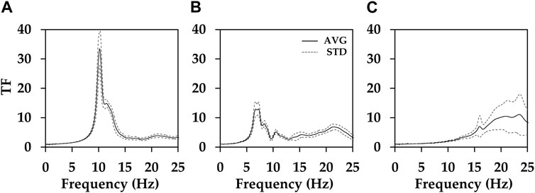
FIGURE 4. Average TF (black solid line) and STD (standard deviation line; grey dotted line) based on data of recorded events at (A) HAMB, (B) IMWB, and (C) YOCB stations.
The fundamental frequency (f0) at IMWB and HAMB stations was 7 and 10 Hz, respectively. The f0 is associated with a velocity contrast in a shallow soil layer (Zhu et al., 2020), and is found first mode of peak in the horizontal-to-vertical spectral ratio (HVSR) (Kwak and Seyhan, 2020). The time-averaged shear-wave velocity to a depth of 30 m (Vs30) was estimated for each of these two stations using the empirical formula suggested by Hassani and Atkinson (2016), and the calculated values were 540 and 676 m s−1, respectively. These estimates correspond to “very dense soil” and “soft rock,” respectively, based on the National Earthquake Hazards Reduction Program Site Classification Standards. In the same way, the f0 at the YOCB station is 15 Hz, with an estimated Vs30 of 872 m s−1, which his classified as “rock”.
3 Collection of field data
Ambient noise data were obtained by segmenting data collected on a day without an event. Figure 5 shows photographs of the 3 stations and their locations. The area of HAMB comprises farmland, and a stream flows in the vicinity of the seismic station. The IMWB station is located on a mountain and is close to a sewage treatment plant. The YOCB station is inside an Automatic Weather Station, on a plain. The three stations have a 100 Hz sampling rate and a Q330HRS recorder (Kinemetrics). IMWB has an STS-2.5 sensor, while HAMB and YOCB both have STS-2.0 sensors (Kinemetrics).
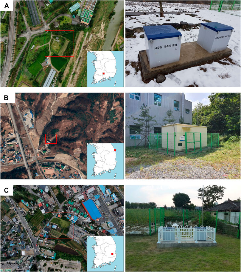
FIGURE 5. Satellite and frontal photographs at (A) HAMB, (B) IMWB, and (C) YOCB stations.
The 24-h waveform at each station was divided into 48 time-windows of 30 min, as artificial noise levels are dependent on the timing of human activity (Roy et al., 2021). Figure 6 compares the ambient noise data recorded by the borehole and surface sensors. The monitoring time for the compared data was 22:10:00–22:11:40 (KST), when there was generally relatively little human activity. Thus, the influence of artificial noise was presumed to be negligible. The noise level in EW direction at the IMWB station was lower than that of the vertical component. As IMWB station was located in the middle of the mountain, a vertical component occurred due to topographical effects (Del Gaudio et al., 2018). We calculated power spectral density (PSD), which are shown in Supplementary Figure S1.
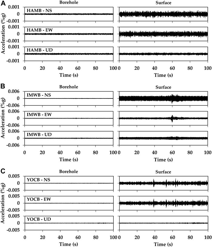
FIGURE 6. Ambient noises were recorded during a 100 s period starting at 22:10:00 (KST). Stations (A) HAMB, (B) IMWB, and (C) YOCB.
4 Data analysis
4.1 Data preprocessing
Data analysis conducted in this study used vibrations recorded by the borehole and surface seismometers at identical time points. Two analyses were performed using the surface-to-borehole vibration ratio. First, the surface-to-borehole ambient noise ratio was calculated. The Fourier amplitude spectrum (FAS) was used to compare the ambient noise; here, only the horizontal components of the noise were considered. The FAS procedure suggested by Ahn et al. (2021) was used as follows:
(1) FFT was applied to the horizontal components of the motions.
(2) FAS was computed in frequencies from 0.1 to 50 Hz, at 0.05 Hz frequency step.
(3) FAS was smoothed by applying Konno and Ohmachi with b = 100.
(4) The geometric mean was calculated between the NS and EW directions from the FAS.
(5) The ratio of the horizontal to vertical components was calculated.
Secondly, to incorporate the influences of the vertical components, HVSR was applied following the FAS. Many studies have shown that the fundamental frequency (f0) of a site can be obtained from the predominant frequency of the ambient vibration HVSR (Sylvette et al., 2006; Guillier et al., 2008; Nagashima et al., 2014; Hassani and Atkinson, 2016; Oubaiche et al., 2016; Kwak and Seyhan, 2018; Ahn et al., 2021). In fact, a Rayleigh wave with an elliptical waveform leads to the disappearance of the vertical amplitude at f0, and the Airy phase of a Love wave leads to the collision of horizontal energy at f0. Using these two phenomena, the reliability of the f0 evaluation method has been theoretically and empirically verified for a simple 1D geological structure, assuming that the peak of the H/V ratio approximates f0 and there is a strong impedance contrast (Sylvette et al., 2006). The interpretation of the HVSR curve is complicated by a lack of understanding regarding the precise composition of the microtremor wavefield, however, the characteristics of the soil layer from the amplitude and frequency could be estimated (Molnar et al., 2022).
4.2 Ambient noise ratio of surface to within motion
Ambient noise is a useful variable because it can easily provide site information about the soil layer. We used the HVSR method, which has the advantage of estimating the site effect without the influence of the source and propagation paths on the response spectrum (Xu and Wang, 2021). Based on this principle, the difference in noise at each depth was analyzed at the same point. Both the HVSR and the differences between components were compared.
Figure 7 illustrates the HVSR of the borehole and surface sensors. The amplitude ratio of HVSR depends on the difference between the horizontal and vertical components. Thus, the HVSR of within-motion at the borehole seismometer is small relative to the ground surface motion. The maximum amplitude at the HAMB station occurs at approximately 10 Hz, which is similar to the results obtained from the TF based on the event. However, the HVSR at the ground surface of IMWB and YOCB stations has a low amplitude, and the dominant frequency is not clearly shown. The vertical component in the IMWB was greater than that at the other stations (Figure 6). Ultimately, it is suggested that the HVSR is relatively low because of the high vertical component noise. The HVSR of YOCB is due to a thin soil layer, as previously analyzed.
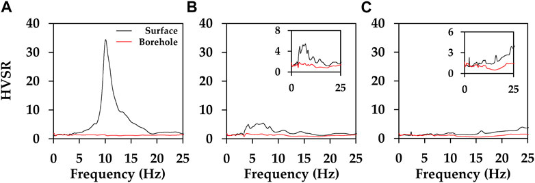
FIGURE 7. Comparison of HVSR for surface and within motions; black solid line is surface motion at the ground surface, and red solid line is motion within the rock layer: stations (A) HAMB, (B) IMWB, and (C) YOCB.
The left column of Figure 8 shows the surface-to-within-motion ratio (SWMR) from the borehole to the surface sensors based on ambient noise. The right column of Figure 8 illustrates the SWMR from the HVSR, termed SWMRHVSR. At the HAMB station, the maximum ratio occurred at a frequency of approximately 10 Hz in both analyses. We found that the resonance frequency that is not visible in the HVSR at IMWB and YOCB stations is slightly clearer in SWMR. The resonance frequency at the IMWB station was determined to be within the range 6.5–7.5 Hz from the NS component. At this time, IMWB seems to show confirmed the amplification of a specific period even in the vertical component due to the topographical effect (Massa et al., 2014; Wang and Sun, 2019). The resonance frequency at the YOCB station was determined to be approximately 16 Hz, based on the event, ambient noise, and HVSR data. The amplitudes of both SWMR and HVSR increased with increasing frequency, while SWMRHVSR did not. This response may have resulted from the overlapping effect of the ambient noise propagation reflected by the bedrock, but we did not identify the cause. The HVSR at the YOCB station is influenced by the hard bedrock layer at shallow depth, overlain by a shallow soil layer. This case has similar characteristics to those reported by Ahn et al. (2021). Such characteristics are common when the soil layer is thin and the two layers have a high impedance ratio (Ghofrani and Atkinson, 2014; Kwak and Seyhan, 2020).
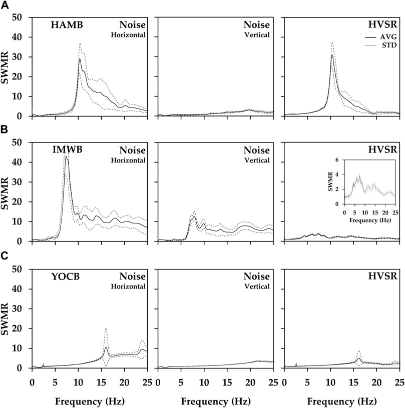
FIGURE 8. Comparison of surface-to-within motion ratio (SWMR) based on ambient noise. Panels on the left represent the horizontal spectral ratios (Hsurface/Hborehole); center panels are the vertical spectral ratios (Vsurface/Vborehole); and right panels are the HVSR ratio (HVSRsurface/HVSRborehole).
Overall, the noise-based SWMR (SWMRn) was higher than or similar to the estimated TF from the event. The gap between the SWMRn and TF is big in the high-frequency domain. This indicates that the ground surface has higher artificial noise levels of unknown high frequencies than the underground. As the high frequencies are steeply attenuated (Peng et al., 2019; Stanko et al., 2020), there is a weak propagation of artificial noise of unknown high frequencies in the underground. For this reason, artificial noise of small amplitude may not be recorded on seismometers 20 m below the ground surface. Additionally, the SWMRHVSR was found to be similar to or lower than the TF identified during the event.
5 Proposed model
In the previous analysis, we confirmed that the noise-based HVSR and SWMR are similar to the event TF in the frequency domain. However, the horizontal amplitude of the ratio of both the HVSR and SWMR depends on the topographical characteristics of the geology (Del Gaudio et al., 2018; Ahn et al., 2021). Therefore, we need an estimation method for calculating TF using SWMR or HVSR.
We proposed a method to correct the horizontal component ratio of between surface and within-rock by the vertical component ratio. The proposed equation is as follow:
where H_Amp and V_Amp are each of horizontal amplitude and vertical amplitude. The subscripts “s" and “wr” indicate the location of the sensor, in either the ground surface or borehole (within rock), respectively. The proposed method combines the noise ratio based on the surface-to-borehole ratio of ambient noise and HVSR results of the surface data.
Figure 9 shows noise-based TF methods, compared with the event-based TF. The proposed model is similar to the TF based on the event and shows excellent performance in the amplitude ratio of the predominant frequency. However, there was a difference in the characteristics at high frequency (20 Hz over). We verified the reliability of the proposed model using recording data in the next chapter.
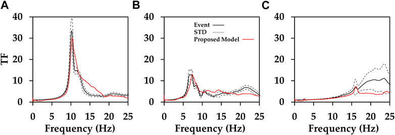
FIGURE 9. Comparison of transfer functions of events (black solid line) and proposed model (red solid line): stations (A) HAMB, (B) IMWB, and (C) YOCB.
6 Results and discussion
6.1 Comparison of numerical method and proposed model
To verify the estimated surface motion based on TF, these values were compared with the ground surface records. First, the borehole record was calculated with the FFT and multiplied by the TF. Then, the calculated frequency value was converted into acceleration time history using inverse FFT again. This allowed us to obtain the ground surface motion.
In Figure 10 , we show the horizontal components of the surface and synthetic seismograms for each station.
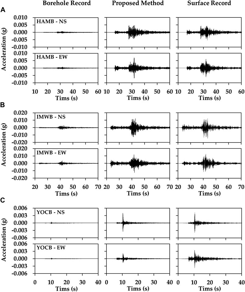
FIGURE 10. Comparison of surface records with proposed model for stations (A) HAMB, (B) IMWB, and (C) YOCB.
Overall, the estimated waveforms were similar to those of the recorded data at the ground surface. Although there were differences between the estimation approach and both methods for ground surface motion, and minor. More specifically, the PGA obtained using the surface motion at the HAMB station was 0.057 m·s−2, whereas that obtained from the proposed model was 0.075 m·s−2 (a difference of 0.018 m·s−2). For the IMWB station, the PGA based on the surface monitoring data was 0.124 m·s−2. The PGA estimated using the proposed model was 0.143 m·s−2. The PGA of the YOCB station at the ground surface was 0.037 m·s−2, whereas the estimated PGA was 0.024 m·s−2 (a difference of 0.013 m·s−2). The PGA gap shows a slight deviation from the recorded surface data.
Figure 11 shows the 5% damped acceleration response spectra of the input and surface ground motions (proposed model and recorded) for the case shown in Figure 2. Overall, the spectral accelerations of ground motions estimated by proposed model were similar to the surface recorded data at all stations. More specifically, the proposed IMWB and YOCB models underestimated the spectral accelerations in the natural frequency region compared to the surface record. Although the difference between the two results is minor, we decided to use the proposed model because it is more reliable than SAC.
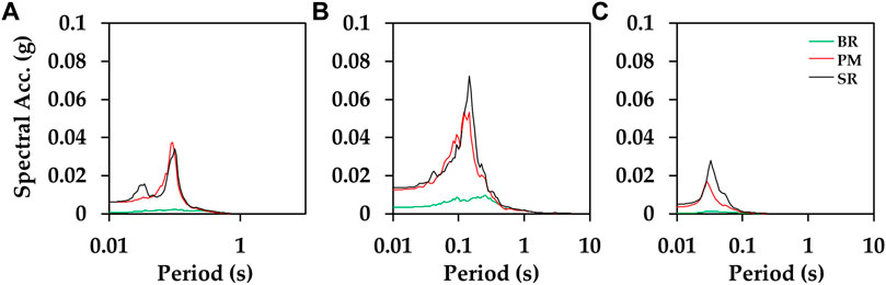
FIGURE 11. Comparison of response spectra: stations (A) HAMB, (B) IMWB, and (C) YOCB. (BR: borehole record; PM: proposed model; SR: surface record).
As our aim to develop a technology that will improve the accuracy of the KMA’s seismic intensity information service, we analyzed the accuracy of the calculated MMI. Figure 12 shows the MMI obtained by applying the proposed model and SAC of the Borcherdt model to the borehole data, as well as the MMI obtained using the surface data. The Borcherdt model is currently being applied to the seismic intensity maps at the KMA. Figure 12A shows MMI obtained by applying the Borcherdt model for the borehole record. To obtain it, the amplification coefficient of Table 3 was applied for each period after the borehole sensor record was frequency-converted. Different MMI conversion equations from the developed KMA model were applied as follows:
where PGA was applied and expressed a unit in cm·s−2.
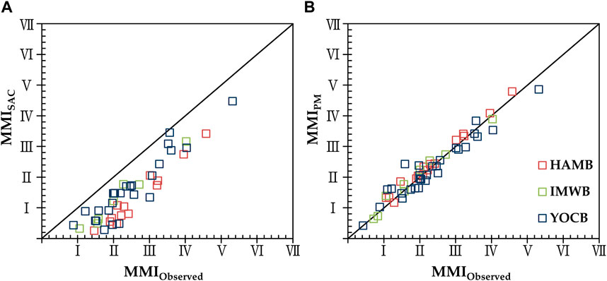
FIGURE 12. Comparison of modified Mercalli intensity (MMI) for site amplitude coefficient (SAC) and proposed model (PM).
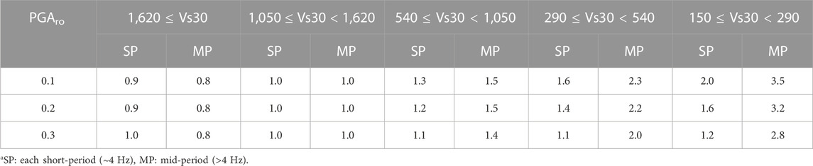
TABLE 3. Site amplification coefficient suggested by Borcherdt (1994).
SAC correction data are expressed as MMISAC and surface data are expressed as MMIObserved. The MMI based on the SAC of the Borcherdt model tended to slightly underestimate that of the surface data. However, the MMI based on the proposed model displayed a 1:1 relationship with the surface data, thereby verifying the outstanding performance of the proposed model.
6.2 Verification
We analyzed noise with three stations and proposed the method of a transfer function to predict. However, the results from the three cases may not be able to represent all stations. Therefore, we additionally searched stations that had one or more events during the period of the temporary surface seismometer operation and used them for a verification case. Although we know the estimated value of Vs30 (Ahn et al., 2021; Cho et al., 2022), there are no shear wave profiles available for the 21 stations used in the verification. For these stations, we collected ambient noise records on both the ground surface and borehole within rocks. We calculated the SWMR and HVSR, which are shown in Supplementary Figure S2. The transfer function was calculated based on the proposed method, as shown in Supplementary Figure S3.
The results of verifying the transfer function based on the proposed method for 45 events in 21 station records are shown in Figure 13. The seismic intensity was calculated by Eqs 4, 5, and the first decimal place was rounded up and expressed in Roman letters. In Figure 13, outside of the square the case of under- or over-predicting the seismic intensity is reported. In the Borcherdt model-based KMA process, the accuracy of the MMI prediction was 7.3 %, while the accuracy of the MMI calculated by the proposed method was 69.1 %. We confirmed that the accuracy of predicting improved by the proposed model.
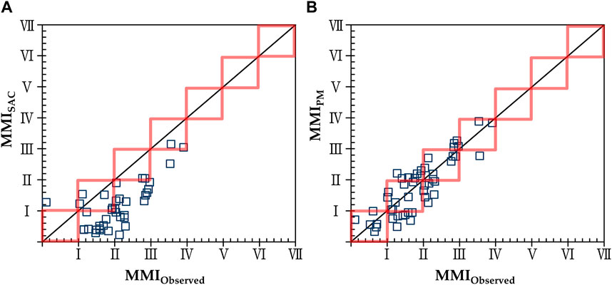
FIGURE 13. Verification of both models. (A) Applied SAC (B) applied the proposed model.
6.3 Automatic computation of seismic intensity
Seismic stations provide seismic intensity information that represents seismic intensity value at the local site and city. If KMA provided the borehole sensor records within motion without correction, the intensity may be sorely underestimated. Therefore, we recommend that the proposed method be applied to each station.
We have designed an automatic computation for seismic intensity, which follows the procedure outlined below:
(1) Extract a record at the 20 m borehole accelerometer sensor after the earthquake (time window default: 300 s)
(2) Apply a noise filtering to the waveform using Choi et al. (2019) method (band-pass filter default: 0.1–50 Hz)
(3) Apply FFT to the event waveform, and multiply the TF (TF is provided as Supplementary Material)
(4) To extract the waveform, apply inverse FFT to the results of 3 step.
(5) Calculate PGA of the waveform, calculated as MMI (using Eqs 4, 5).
7 Conclusion
The aim of this study was to estimate horizontal direction waves recorded by in-borehole seismometers in order to accurately estimate seismic intensity at the ground surface. The proposed model is based on ambient noise data collected from both surface and borehole sensors.
To this end, the fundamental frequency of the soil layer was determined based on the TF values of the event, ambient noise, and HVSR without performing ground surveys. At locations with both borehole and surface sensors, the natural frequency of the soil layer can be calculated via a surface-to-within-motion ratio based on the HVSR.
At high frequencies, the SWMR was generally high with respect to ambient noise and relatively low for SWMRHVSR. However, the noise-based TF calculated using the proposed model exhibited a trend similar to the TF of the event analysis. The TF values obtained via event analysis mostly came from intact ground data, which allowed for the analysis of linear behavior. Thus, the model proposed in this study did not consider non-linear amplification; further studies should therefore address this consideration.
The proposed approach requires a temporary seismometer to be installed on the surface for 1 day. The TF can be calculated using the obtained ambient noise. If we perform frequency domain response analysis based on the TF, we can estimate the acceleration time history on the surface. This approach has a significant advantage of not requiring additional geotechnical surveys. However, the present study only analyzed three stations, and so the approach could be further improved through additional research.
The validation of the proposed model showed that it can be applied to borehole data to estimate ground surface vibrations. Although the exact waveform generated by the model did not always exactly recreate observational data, the model delivered PGA values with lower errors than those obtained using the site coefficient. Therefore, this model represents a significant improvement in the accuracy of seismic intensity estimation (for which the site coefficient is currently employed). Using the TF developed in this study could enable reliable seismic intensity estimations to be obtained while operating borehole data; this would be particularly advantageous at stations that lack surface seismometers such as KMA.
Finally, the automatic calculation process based on the proposed method can be applied in real-time. Most earthquake information is provided in a brief time immediately after an event. At this time, the accuracy of the information affects the reliability of the institution or the government and future research. Therefore, the provided automated real-time MMI processing will be very useful.
Data availability statement
The original contributions presented in the study are included in the article/Supplementary Material, further inquiries can be directed to the corresponding author.
Author contributions
DL contributed to the writing of the manuscript and the analysis and processing of the data. J-KA supervised the study, contributed to its conceptualization and writing, and contributed to the design and analysis of the data. All the authors have read and agreed to the published version of the manuscript.
Funding
This study was supported by Development of Earthquake Information Production Technology (grant number KMA 2022-02121).
Acknowledgments
The authors are grateful to staff of the KMA Earthquake and Volcano Research Division.
Conflict of interest
The authors declare that the research was conducted in the absence of any commercial or financial relationships that could be construed as a potential conflict of interest.
Publisher’s note
All claims expressed in this article are solely those of the authors and do not necessarily represent those of their affiliated organizations, or those of the publisher, the editors and the reviewers. Any product that may be evaluated in this article, or claim that may be made by its manufacturer, is not guaranteed or endorsed by the publisher.
Author disclaimer
The opinions, findings, and conclusion expressed in this material are those of the authors and do not necessarily reflect those of the KMA.
Supplementary material
The Supplementary Material for this article can be found online at: https://www.frontiersin.org/articles/10.3389/feart.2023.1047667/full#supplementary-material
Abbreviations
KMA, Korea Meteorological Administration; SAC, Site amplification coefficient; MMI, Modified Mercalli intensity; MASW, Multichannel analysis of surface waves; 1D, One-dimensional; PGA, Peak ground acceleration; TF, Transfer function; FFT, Fast Fourier transform; HVSR, Horizontal-to-vertical spectral ratio; FAS, Fourier amplitude spectrum; SWMR, Surface-to-within-motion ratio.
References
Ahn, J. K., Kwak, D., and Kim, H. S. (2021). Estimating VS30 at Korean Peninsular seismic observatory stations using HVSR of event records. Soil Dyn. Earthq. Eng. 146, 106650. doi:10.1016/j.soildyn.2021.106650
Albarello, D., and Lunedei, E. (2010). Alternative interpretations of horizontal to vertical spectral ratios of ambient vibrations: New insights from theoretical modeling. Bull. Earthq. Eng. 8 (3), 519–534. doi:10.1007/s10518-009-9110-0
Asten, M. W., and Hayashi, K. (2018). Application of the spatial auto-correlation method for shear-wave velocity studies using ambient noise. Surv. Geophys. 39, 633–659. doi:10.1007/s10712-018-9474-2
Borcherdt, R. D. (1994). Estimates of site-dependent response spectra for design (methodology and justification). Earthq. Spectra 10 (4), 617–653. doi:10.1193/1.1585791
BSSC (1997). NEHRP recommended seismic provisions for new buildings and other structures, FEMA 302 Part 1 (provisions). Washington DC: Building Seismic Safety Council.
Cho, H. I., Lee, M. G., Ahn, J. K., Sun, C. G., and Kim, H. S. (2022). Site flat file of Korea Meteorological Administration’s seismic stations in Korea. Bull. Earthq. Eng. 20, 5775–5795. doi:10.1007/s10518-022-01418-8
Choi, I., Ahn, J. K., and Kwak, D. (2019). A fundamental study on the database of response history for historical earthquake records on the Korean peninsula (Korea). J. KSCE. 39 (6), 821–8310. doi:10.12652/Ksce.2019.39.6.0821
Cultrera, G., De Rubeis, V., Theodoulidis, N., Cadet, H., and Bard, P. (2014). Statistical correlation of earthquake and ambient noise spectral ratios. Bull. Earthq. Eng. 12, 1493–1514. doi:10.1007/s10518-013-9576-7
Del Gaudio, V., Luo, Y., Wang, Y., and Wasowski, J. (2018). Using ambient noise to characterise seismic slope response: The case of qiaozhuang peri-urban hillslopes (sichuan, China). Eng. Geol. 246, 374–390. doi:10.1016/j.enggeo.2018.10.008
Dobry, R., Borcherdt, R. D., Crouse, C. B., Idriss, I. M., Joyner, W. B., Martin, G. R., et al. (2000). New site coefficients and site classification system used in recent building seismic code provisions. Earthq. Spectra 16 (1), 41–67. doi:10.1193/1.1586082
García-Fernández, M., and Jiménez, M. J. (2012). Site characterization in the Vega Baja, SE Spain, using ambient-noise H/V analysis. Bull. Earthq. Eng. 10 (4), 1163–1191. doi:10.1007/s10518-012-9351-1
Ghofrani, H., and Atkinson, G. M. (2014). Site condition evaluation using horizontal-to-vertical response spectral ratios of earthquakes in the NGA-West 2 and Japanese databases. Soil Dyn. Earthq. Eng. 67, 30–43. doi:10.1016/j.soildyn.2014.08.015
Guillier, B., Atakan, K., Chatelain, J. L., Havskov, J., Ohrnberger, M., Cara, F., et al. (2008). Influence of instruments on the H/V spectral ratios of ambient vibrations. Bull. Earthq. Eng. 6, 3–31. doi:10.1007/s10518-007-9039-0
Hassani, B., and Atkinson, G. M. (2016). Applicability of the site fundamental frequency as a VS30 proxy for central and eastern north America. Bull. Seismol. Soc. Am. 106 (2), 653–664. doi:10.1785/0120150259
Jang, D., Ahn, J. K., Kim, T. W., and Kwak, D. (2023). Linearly combined ground motion model using quadratic programming for low to mid-size seismicity region: South Korea. Front. Earth Sci. 10, 2531. doi:10.3389/feart.2022.1067802
Konno, K., and Ohmachi, T. (1998). Ground-motion characteristics estimated from spectral ratio between horizontal and vertical components of microtremor. Bull. Seismol. Soc. Am. 88 (1), 228–241. doi:10.1785/BSSA0880010228
Kwak, D., Ahn, J. K., Seo, H., Kang, S., and Kim, B. (2022). Single-path ground motion amplifications during the 2020 Haenam, South Korea, swarm. Bull. Earthq. Eng. 20, 4937–4959. doi:10.1007/s10518-022-01386-z
Kwak, D., and Seyhan, E. (2018). “Development of peak frequency-site condition correlation models using H/V spectral ratio,” in Proceedings of the geotechnical earthquake engineering and soil dynamics V (Reston, VA: ASCE Library), 340–347. doi:10.1061/9780784481462.033
Kwak, D., and Seyhan, E. (2020). Two-stage nonlinear site amplification modeling for Japan with VS30 and fundamental frequency dependency. Earthq. Spectra. 36 (3), 1359–1385. doi:10.1177/8755293020907920
Lai, T. S., Chao, W. A., and Wu, Y. M. (2022). A local magnitude scale from borehole recordings with site correction of the surface to downhole. Seismol. Res. Lett. 93 (3), 1524–1531. doi:10.1785/0220210252
Manandhar, S., Cho, H. I., and Kim, D. S. (2018). Site classification system and site coefficients for shallow bedrock sites in Korea. J. Earthq. Eng. 22 (7), 1259–1284. doi:10.1080/13632469.2016.1277570
Massa, M., Barani, S., and Lovati, S. (2014). Overview of topographic effects based on experimental observations: Meaning, causes and possible interpretations. Geophys. J. Int. 197 (3), 1537–1550. doi:10.1093/gji/ggt341
McCann, M. W., Sauter, F., and Shah, H. C. (1980). A technical note on PGA-intensity relations with applications to damage estimation. Bull. Seismol. Soc. Am. 70 (2), 631–637. doi:10.1785/BSSA0700020631
Moisidi, M., Vallianatos, F., Kershaw, S., and Collins, P. (2015). Seismic site characterization of the kastelli (kissamos) basin in northwest crete (Greece): Assessments using ambient noise recordings. Bull. Earthq. Eng. 13, 725–753. doi:10.1007/s10518-014-9647-4
Molnar, S., Sirohey, A., Assaf, J., Bard, P. Y., Castellaro, S., Cornou, C., et al. (2022). A review of the microtremor horizontal-to-vertical spectral ratio (MHVSR) method. J. Seismol. 26, 653–685. doi:10.1007/s10950-021-10062-9
Nagashima, F., Matsushima, S., Kawase, H., Sanchez-Sesma, F. J., Hayakawa, T., Satoh, T., et al. (2014). Application of horizontal-to-vertical spectral ratios of earthquake ground motions to identify subsurface structures at and around the K-NET site in Tohoku, Japan. Bull. Seismol. Soc. Am. 104 (5), 2288–2302. doi:10.1785/0120130219
Oubaiche, E., Chatelain, J. L., Hellel, M., Wathelet, M., Machane, D., Bensalem, R., et al. (2016). The relationship between ambient vibration H/V and SH transfer function: Some experimental results. Seismol. Res. Lett. 87 (5), 1112–1119. doi:10.1785/0220160113
Padgett, J. E., and DesRoches, R. (2008). Methodology for the development of analytical fragility curves for retrofitted bridges. Earthq. Eng. Struct. Dyn. 37 (8), 1157–1174. doi:10.1002/eqe.801
Park, D., and Hashash, Y. M. A. (2004). Soil damping formulation in nonlinear time domain site response analysis. J. Earthq. Eng. 8 (2), 249–274. doi:10.1080/13632460409350489
Park, E. H., Lee, J. M., and Kim, W. (2011). Performance of the southern Korean Peninsula seismograph network and refinement of hypocentral parameters of local earthquakes, 2004–2008. Geosci. J. 15 (1), 83–93. doi:10.1007/s12303-011-0001-4
Peng, Y., Su, Y., Wu, L., and Chen, C. (2019). Study on the attenuation characteristics of seismic wave energy induced by underwater drilling and blasting. Shock Vib. 2019, 1–13. doi:10.1155/2019/4367698
Roy, K. S., Sharma, J., Kumar, S., and Kumar, M. R. (2021). Effect of coronavirus lockdowns on the ambient seismic noise levels in Gujarat, northwest India. Sci. Rep. 11 (1), 7148. doi:10.1038/s41598-021-86557-9
Shinozuka, M., Feng, M. Q., Lee, J., and Naganuma, T. (2000). Statistical analysis of fragility curves. J. Eng. Mech. ASCE 126 (12), 1224–1231. doi:10.1061/(asce)0733-9399(2000)126:12(1224)
Stanko, D., Markušić, S., Korbar, T., and Ivančić, J. (2020). Estimation of the high-frequency attenuation parameter kappa for the Zagreb (Croatia) seismic stations. Appl. Sci. 10 (24), 8974. doi:10.3390/app10248974
Sylvette, B. C., Cécile, C., Pierre-Yves, B., Fabrice, C., Peter, M., Jozef, K., et al. (2006). H/V ratio: A tool for site effects evaluation. Results from 1-D noise simulations. Geophys, J. Int. 167 (2), 827–837. doi:10.1111/j.1365-246X.2006.03154.x
Wang, S., and Sun, X. (2019). Topography effect on ambient noise tomography using a dense seismic array. Earthq. Sci. 31 (5-6), 291–300. doi:10.29382/eqs-2018-0291-9
Xu, R., and Wang, L. (2021). The horizontal-to-vertical spectral ratio and its applications. EURASIP J. Adv. Signal Process 2021, 75. doi:10.1186/s13634-021-00765-z
Keywords: site effect, site amplification, transfer function, within rock records, borehole seismometer, ambient noise
Citation: Lim D and Ahn J-K (2023) Horizontal seismic wave at ground surface from transfer function based on ambient noise. Front. Earth Sci. 11:1047667. doi: 10.3389/feart.2023.1047667
Received: 18 September 2022; Accepted: 23 February 2023;
Published: 16 March 2023.
Edited by:
Vincenzo Convertito, National Institute of Geophysics and Volcanology (INGV), ItalyReviewed by:
Lucia Nardone, Istituto Nazionale di Geofisica e Vulcanologia (INGV), ItalySeokho Jeong, Changwon National University, Republic of Korea
Copyright © 2023 Lim and Ahn. This is an open-access article distributed under the terms of the Creative Commons Attribution License (CC BY). The use, distribution or reproduction in other forums is permitted, provided the original author(s) and the copyright owner(s) are credited and that the original publication in this journal is cited, in accordance with accepted academic practice. No use, distribution or reproduction is permitted which does not comply with these terms.
*Correspondence: Jae-Kwang Ahn, cHJvcGprQGtvcmVhLmty, cHJvcGprQGdtYWlsLmNvbQ==