 M. Pischiutta
 S. Petrosino
 R. Nappi
94% of researchers rate our articles as excellent or good
Learn more about the work of our research integrity team to safeguard the quality of each article we publish.
Find out more
BRIEF RESEARCH REPORT article
Front. Earth Sci., 12 December 2022
Sec. Solid Earth Geophysics
Volume 10 - 2022 | https://doi.org/10.3389/feart.2022.999222
This article is part of the Research TopicWomen in Science: Seismology 2022View all 6 articles
In this paper, we investigated ground motion directional amplification and horizontal polarization using ambient noise measurements performed in the northern sector of Ischia Island which suffered damage (VIII EMS) during the 21 August 2017, Md 4.0 earthquake. Over 70 temporary seismic stations were installed by the INGV EMERSITO task force, whose aim is to monitor site effects after damaging earthquakes in Italy. To investigate ground motion directional amplification effects, we have applied three different techniques, testing their performance: the HVSR calculation by rotating the two horizontal components, the covariance matrix analysis, and time–frequency domain polarization analysis. These techniques resulted in coherent outcomes, highlighting the occurrence of directional amplification and polarization effects in two main sectors of the investigated area. Our results suggest an interesting pattern for ground motion polarization, that is mainly controlled by recent fault activity and hydrothermal fluid circulation characterizing the northern sector of the Ischia Island.
• Directional amplification and ground motion amplification are investigated at the Ischia Island after the 21 August 2017, Md 4.0 earthquake.
• Robust results were obtained by applying three analysis techniques in time and frequency domains, revealing a good agreement.
• The directional amplification pattern and polarization are mainly controlled by recent fault activity and hydrothermal fluid circulation.
Directional amplification refers to site amplification in the frequency domain mainly occurring along a site-dependent azimuth. Such effects have recently been observed at rock sites at frequencies of engineering interest (1–10 Hz), with the number of observations increasing worldwide. The main signature of this effect is that the signal is amplified along a site-specific azimuth in the horizontal plane, and the horizontal components of ground motion show amplitudes exceeding three times the vertical component (Pischiutta et al., 2012). Along the amplified azimuth, the horizontal ground motion amplitude exceeds 100% of the complementary azimuth angle. In the time domain, directional amplification corresponds to linearly polarized ground motion.
Such effects are often consistently observed on both earthquake wavefield and ambient noise, suggesting that the local subsoil geological structure plays the main role, rather than being related to the earthquake/noise source and/or path. Moreover, it was proven that directional amplification effects could unexpectedly involve relevant areal extents, up to several kilometers wide (Pischiutta et al., 2014), and a high number of rock sites among stations of permanent seismic networks (Burjànek et al., 2014a; Burjànek et al., 2014b; Pischiutta et al., 2018).
Directional amplification has been observed so far in different geological frameworks, such as 1) fractured rock slopes/gravitational instabilities/landslides (Del Gaudio and Wasowski, 2007; Moore et al., 2011, 2018; Burjánek et al., 2012; Häusler et al., 2019), 2) fault damage zones (Pischiutta et al., 2012; Hailemikael et al., 2016; Di Giulio et al., 2019; Vignaroli et al., 2019), and 3) the volcanic environment (Falsaperla et al., 2010; Petrosino et al., 2012; Panzera et al., 2020; Petrosino & De Siena, 2021).
On fractured rock slopes, maximum amplification and ground motion polarization transversal to large open fractures associated with the movement of the slope instability are observed in several papers (Burjánek et al., 2010 and many others). Recently, Burjanek and Kleinbrod (2019) successfully reproduced the observed transfer function on fractured rock slopes by using three-dimensional numerical simulations of seismic wave propagation. They confirmed that compliant fractures can generate polarized ground motion and maximum amplification transverse to their strike, the effect being primarily controlled by the stiffness, depth, number of fractures, and inertial mass of the fractured rock.
Similar effects were also observed across fault damage zones (FDZs), with maximum amplification and polarization transversal to the predominant fracture field held open by the acting stress field (Martino et al., 2006; Rigano et al., 2008; Di Giulio et al., 2009; Marzorati et al., 2011; Pischiutta et al., 2012; Vignaroli et al., 2019; Panzera et al., 2014; Panzera et al., 2020), such as due to stiffness anisotropy. This interpretation was confirmed by comparison with S-wave splitting studies (Pischiutta et al., 2015; Panzera et al., 2017) and by the controlled-source seismic experiment involving polarized seismic sources (Di Giulio et al., 2019).
However, we remark that across fault zones, apart from directional amplification and polarization transversal to the predominant fracture field, another well-known effect can occur. It involves trapped waves by damaged rocks with high crack density (Ben-Zion & Sammis 2003, and references therein), and it is caused by the constructive interference of critically reflected phases (Ben-Zion & Aki, 1990; Li & Leary 1990; Li et al., 1997; Spudich & Olsen, 2001). This effect results in the time domain in polarization parallel to the fault strike and in the frequency domain, to directional amplification in a frequency band depending on the velocity contrast between the fault zone and host rock.
Furthermore, in the volcanic environment, recent studies investigating temporal variations of ground motion polarization suggested interesting outcomes. In these frameworks, the presence of fluid flow in rock fractures generates local seismic noise that progressively intensifies and causes a loss of polarization (depolarization). This was mostly observed at stations on fault zones where, in the absence of fluid flows, ground motion exhibits polarization effects (Petrosino and De Siena, 2021). Therefore, observed changes in polarization strength patterns allowed Petrosino and De Siena (2021) to map the stress build-up and release throughout time, providing a technique to monitor fluid-driven processes at stressed volcanoes.
In this paper, we study ground motion directional amplification and polarization effects in Ischia Island, using ambient noise recordings. We apply three different techniques, testing their performance: the horizontal-to-vertical spectral ratio (HVSR) calculation by rotating the two horizontal components (Nakamura, 1989; Spudich et al., 1996), the covariance matrix analysis (Kanasewich, 1981; Jurkevics, 1988), and the time–frequency domain polarization analysis (Vidale, 1986; Burjànek et al., 2010).
Ischia is an active volcanic island on the northwestern side of the Gulf of Naples and represents the subaerial portion of a volcanic complex that was active since at least 150 ka B.P. (Vezzoli, 1998). The island is characterized by numerous effusive and explosive eruptions, with alternating periods of quiescence (Tibaldi and Vezzoli, 1998; Vezzoli, 1998; Bruno et al., 2002; Tibaldi and Vezzoli, 2004; de Vita et al., 2010). The activity was dominated by the caldera-forming Green Tuff eruption of 55 ka B.P, followed by at least 30 ka B.P. by block resurgence within the caldera that finally created Mt. Epomeo (787 m. a.s.l.) with an overall uplift of ca. 900 m. The last volcanic activity period started 10 ka B.P, with eruptions in the eastern sector of the island including the most recent eruption of Arso in 1302 (de Vita et al., 2010).
Ischia is composed of volcanic rocks, epiclastic deposits, and subordinate terrigenous sediments, reflecting a complex history of alternating constructive and destructive phases. Lava and tuffs are the more ancient rock of the island that comprise the substratum for all the younger overlaying volcano-sedimentary successions (Figure 1).
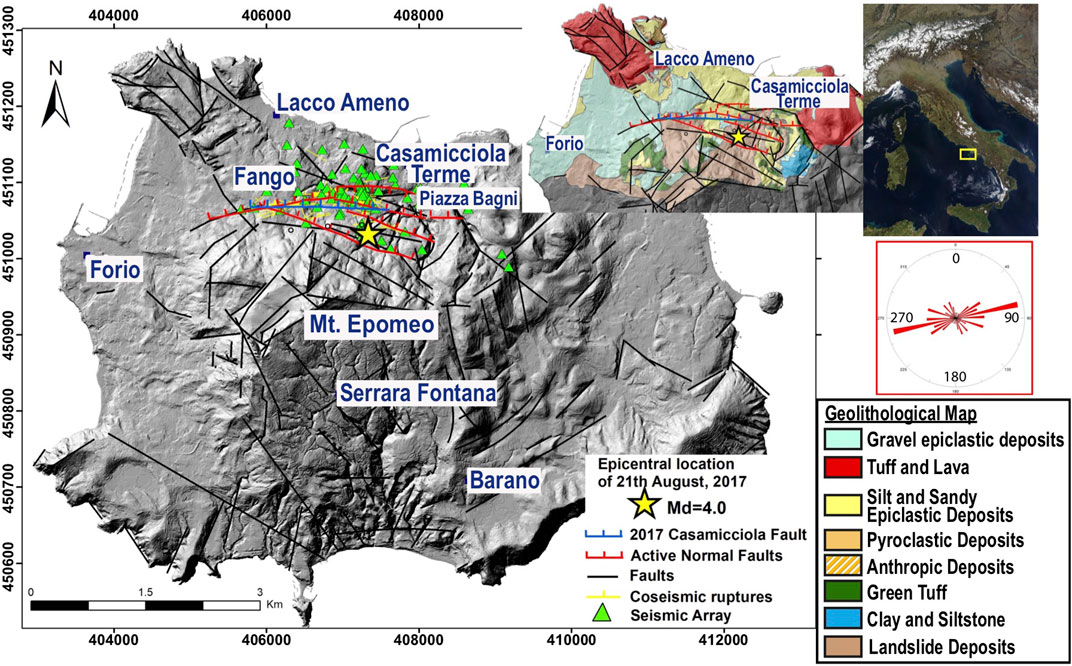
FIGURE 1. Geostructural sketch map on the shaded relief in UTM WGS-84 geographic coordinates by Nappi et al. (2010). The featured stratigraphic units are simplified from Sbrana et al. (2018). Faults (in black) are from Acocella and Funiciello (1999) and de Vita et al. (2010), and geomorphological lineaments (in black), from Nappi et al. (2010); active normal faults (red lines, marks on down-thrown side) are from Vezzoli (1998) and Tibaldi and Vezzoli (1998); the coseismic ruptures (yellow lines) and causative fault (blue line) of 2017 earthquake and rose diagram of the same are from Nappi et al. (2018b); surface trace of the 2017 earthquake causative fault (blue line) from this paper; and the 21 August 2017 mainshock (the yellow biggest star) is from https://terremoti.ov.ingv.it/gossip/ischia/2017/index.html.
On 21 August 2017, a Md 4.0 (Mw 3.9) 1.4 km deep earthquake struck Casamicciola Terme village, with the hypocenter located inside the graben at the base of the N flank of Mt. Epomeo. In this few square kilometer-wide graben, seismic events have repeatedly occurred throughout history with similar characteristics (Cubellis and Luongo, 1998; Alessio et al., 1999). This graben formed in the Holocene as a consequence of the extensional tectonic deformation and therefore, represents the stratigraphic and morphological trace of active tectonics (Rittman, 1930; Vezzoli, 1998; Tibaldi and Vezzoli, 1998; Sbrana et al., 2018). It represents the long-term cumulative expression of repeated earthquake surface faulting along two main systems (Nappi et al., 2018a; Nappi et al., 2018b): 1) a parallel system of ENE-striking, 60°–85° N dipping synthetic faults, overall along the master fault on the resurgent Mt. Epomeo N flank (slip-rate exceeding 3 cm/yr between 33 kyr B.P and the present); and 2) a secondary antithetic, southward dipping normal fault system.
Nappi et al. (2021) performed a detailed study of coseismic effects and extensional faults, with the aim of formulating a hypothesis on the seismogenetic source model for 2017 Casamicciola earthquake, even considering other previous models based on deformation data (Sepe et al., 2007; Calrderoni et al., 2019). They suggested that the 21 August earthquake was caused by reactivation of the E–W normal fault system that is associated with the Holocene uplift of the Mt Epomeo N flank (blue lines in Figure 1). Its geometric characteristics are similar to the causative faults of historical strong earthquakes in the same area during 18–19 centuries (1762, 1767, 1796, 1828, 1881, and 1883), with maximum observed MCS intensities ranging between VII and XI (Selva et al., 2021 and references therein), and very strong attenuation with increasing epicentral distance (Nappi et al., 2021). The high resurgence rate combined with the seismic activity and the hydrothermal system has produced steep slopes on the flanks of Mt. Epomeo, exposing the ignimbrites and the overlying marine sediments to subaerial slope instabilities, that favored the development of shallow mass movements, debris avalanches, debris flow, and lahars (Figure 1) (Del Prete and Mele, 1999, 2006; Della Seta et al., 2015).
We use data collected by 75 temporary seismic stations installed by the INGV EMERSITO task force in the northern sector of Ischia Island, in the localities of Casamicciola Terme, Fango, and Lacco Ameno (green triangles in Figure 1). They are composed of a Lennartz 5 s triaxial velocimetric sensor coupled with Reftek RT130 or Marslite digitizers. At each site, seismic noise data were recorded for at least 1 h (Vassallo et al., 2018a; Vassallo et al., 2018b; Nardone et al., 2022). Further details such as geographical coordinates and date of noise acquisition are reported in Supplementary Table S1.
In this paper, we analyze ambient noise recordings, implementing three different techniques to investigate directional motion. They have been used so far for similar purposes and include 1) the horizontal-to-vertical spectral ratios (HVSRs) after rotating the horizontal components, operating in the frequency domain to detect directional amplification peaks (first used in Spudich et al., 1996), 2) the covariance matrix analysis (Kanasewich 1981; Jurkevics 1988) performed in the time domain after bandpass filtering the signal in selected frequency bands, and 3) the time–frequency analysis working both in the time and frequency domains (Vidale 1986). The combined use of these three different techniques is very important to obtain an overall, robust, and complete description of the observed effects and to overcome the limitations intrinsic to each one. As an example, the HVSR technique can be “non-informative” in some cases (e.g., in the presence of lateral and vertical heterogeneities or velocity inversion), due to the occurrence of amplification on the vertical component of motion. Indeed, in the covariance matrix analysis, signals need to be bandpass filtered; thus, it cannot furnish a complete description of the effects in all frequency ranges. Conversely, the time–frequency polarization analysis led to description of the effect versus frequency, but it is hard to interpret the results using the quantitative criterion, as we will demonstrate in the next sections for the other two methods.
We use the following analysis flow:
1) We use rotated HVSRs to get a grasp on the directional amplification effect, quantitatively defining its pattern through several parameters (Section 3.1).
2) We apply the time-domain covariance matrix technique, bandpass filtering signals in the frequency bands 0.2–0.8 and 1–5 Hz, where the main HVSR peaks fall, obtaining an estimate at each station of polarization strength and mean azimuth (Section 3.2).
3) Finally, the time–frequency technique was used to validate the results using the two previous techniques in terms of the polarization azimuth (Section 3.3).
The HVSRs are calculated at each station following the technique proposed by Spudich et al. (1996) to study ground motion horizontal polarization, which was subsequently widely exploited (Cultrera et al., 2003; Rigano et al., 2008; Pischiutta. 2010). We used the package Geopsy (Wathelet, 2005). In order to analyze the stationary parts and eliminate non-stationary disturbances associated with very close disturbances, we selected time windows using the antitrigger algorithm proposed in the SESAME guidelines (SESAME, 2004). We ensured the availability of at least 30 time windows at each station.
The calculation of HVSRs was then performed by rotating the two horizontal components by steps of 10° from 0° to 180°. For each rotated component, we considered a window length of 120 s, 5% tapered, filtered with a fourth-order Butterworth filter in the frequency range 0.1–25 Hz, and smoothed with the Konno–Ohmachi algorithm (b=20, Konno and Ohmachi, 1998).
In Figure 2, we show directional amplification estimated through the HVSR at two exemplificative stations, ESI35 and ESI17. In the Supplementary Material, we also furnish results at the other stations. The HVSR curves are plotted separately for each rotation angle (panels a1 and c1). They are also graphed using a contour plot (panels b1 and d1), the x-scale represents the frequency; the y-scale, the rotation angle; and the color scale is related to amplitude levels. In this way, HVSRs show to what extent horizontal motion is amplified compared to vertical motion, as a function of the frequency and direction of motion allowing the detection of the frequency band where ground motion tends to be mostly horizontal.
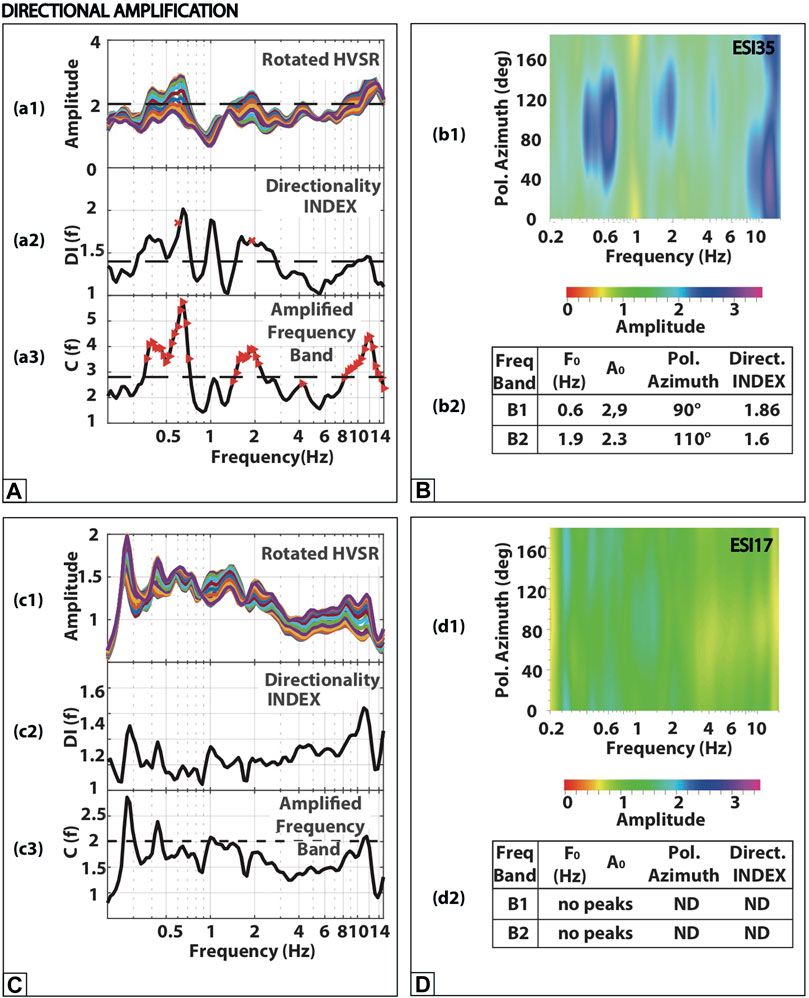
FIGURE 2. Results at two exemplificative stations for directional amplification estimated through the HVSR by rotating the two horizontal components at steps of 10° from 0° to 180°: ESI35 (clear peaks), panels (A,B), and ESI17 (no peaks), panels (C,D). HVSR curves obtained separately for each rotation angle are graphed in panels a1 and c1. Rotated HVSRs are also plotted using a contour plot: the x-scale representing frequency; the y-scale, the rotation angle; and the color scale is related to amplitude levels (panels b1 and d1). In this way, HVSRs show to what extent horizontal motion is amplified, compared to vertical motion, as a function of frequency and direction of motion allowing the detection of the frequency band, where ground motion tends to be mostly horizontal. We apply an automatic criterion to interpret results and distinguish directional peaks (Pischiutta et al., 2018). We use the directionality index (DI) (f) (Eq. 1), defined as the ratio between the maximum and minimum amplitude values given at the frequency peak (F0) by all rotation angles (panels a2 and c2). To assess the frequency band where the largest amplification falls, we consider the parameter C (f), as defined in Eq. 3 (panels a3 and c3). Finally, the directional amplification pattern at each station is defined through the frequency band, F0; maximum amplitude (A0); polarization azimuth; and directionality index (DI). Such parameters obtained for the two exemplificative stations are summarized in panels b2 and d2.
At first, we found the largest amplitude value (A0) on HVSR curves and read the associated frequency value, that is the frequency peak (F0). In accordance with the SESAME guidelines (2004), we considered an Amax of HVSRs higher than 2 as the basic condition for ground motion amplification. Then, following Pischiutta et al. (2018) and considering the minimum (MinHV) and maximum (MaxHV) amplitude values given at F0 by all rotation angles, we automatically estimate at each station:
1) The directionality index, defined as follows:
The directionality index was proposed by Pischiutta et al. (2018) to distinguish whether a peak is directional or uniform in the CRISP INGV database (http://crisp.ingv.it), involving all stations of the Italian seismic network. They considered a threshold of 1.5 for DI [that is called “function B (f)” in their work], based on authors’ practice and common experience. However, in this work, due to comparison with other techniques, we chose to downgrade this threshold to 1.4.
2) The polarization azimuth (i.e., the rotation angle associated with Amax).
3) The frequency band where the largest amplification falls. It is defined using the parameter C (f), given by
using the portion of C(f) where
Further details about the criterion used to objectively interpret the results of HVSR analysis involving DI (f) and C(f) can be found in Pischiutta et al. (2018).
Station ESI35 shows two peaks at 0.6 and 1.9 Hz, respectively, with amplitudes over 2. They are associated with DI over 1.4, and therefore, this station is considered to be affected by directional amplification. Polarization azimuth values are 90° and 110° for F0 of 0.6 and 1.9 Hz, respectively. These directions correspond to the maximum amplitude values at the two peak frequencies, and therefore, there is no associated standard deviation.
On the contrary, station ESI17 is not affected by amplification effects, and HVSR amplitudes are lower than two in the whole considered frequency band 0.2–15 Hz. Therefore, in the absence of peaks, the remnant parameters are not defined (ND).
In order to assess HVSR result variability over small distances, we also processed data acquired by four 2D seismic arrays, whose data and results are described in detail in a complementary paper by Nardone et al. (2022). Stations in each array acquired a simultaneous signal for at least 90 min during daytime, with a sampling rate of 250 Hz. Their locations and results in terms of rotated HVSRs are furnished in the Supplementary Data Sheet S1.
Ambient noise recordings at each site were filtered by applying a bandpass a-causal Butterworth filter in two frequency bands, 0.2–0.8 and 1–5 Hz, chosen on the basis of HVSR results. Then, we applied the covariance matrix method (Kanasewich 1981; Jurkevics, 1988) to the three-component filtered signals using a sliding time window whose length was fixed to contain 1.5 wave cycles of the maximum period, with an overlap of 75%. In each window, the polarization ellipsoid is estimated through the eigenvalues and eigenvectors of the covariance matrix by solving the algebraic eigenvalue problem. They correspond, respectively, to the length and orientation of the polarization ellipsoid, thus defining the polarization vector in 3D (Figure 2 in Pischiutta et al., 2015). According to Jurkevics (1988), the polarization ellipsoid is characterized by three parameters:
- rectilinearity R, defined as
with
- Azimuth AZ of the polarization vector, defined as the angle between the projection on the horizontal plane of the polarization vector and north, measured clockwise.
- Incidence angle I between the polarization vector and the vertical axis: 90° angles indicate horizontal propagation, whereas 0° angles correspond to the vertical incidence.
In order to select polarization azimuth values associated with a horizontal and linear ground motion, we apply a hierarchical criterion proposed by Pischiutta et al. (2012), mainly consisting of :
- Exclusion from statistics values of AZ for which R < 0.5 and I < 45° (that means sub-spherical and nearly vertical polarization ellipsoids).
- Linearly normalizing between 0 and 1 the R and I values ranging in the intervals 0.5 ≤ R < 1 and 45° ≤ I < 90°, making linearized values Rlin and Ilin.
- Calculation of a weight value WH in each time window given by
We use as a threshold
Finally, in order to quantify the spread of the azimuthal distribution of the polarization vector, we estimated a statistical parameter, and the resultant vector length is defined as follows:
where
The results at two exemplificative stations (ESI35 and ESI17) are shown in Figure 3. Histograms of polarization azimuth values are obtained in the frequency bands 0.2–0.8 Hz (panels a1 and c1) and 1–5 Hz (panels b1 and d1). Similarly, in panels a2, b2, c2, and d2, we also add histograms of the rectilinearity values, given by Eq. 4. We stress that in both frequency bands, at station ESI35, polarization azimuth values are concentrated around a mean (N88°±19° and N104°±25° for the bands 0.2–0.8 and 1–5 Hz, respectively). In fact, the RL parameter in both the bands is higher than 0.6. Conversely, at station ESI17, polarization azimuth values are spread (RL ≤ 0.4); therefore, a mean polarization azimuth cannot be defined. We finally stress that at ESI17, rectilinearity values are lower than those at station ESI35, confirming that ESI17 is not affected by ground motion horizontal polarization effects.
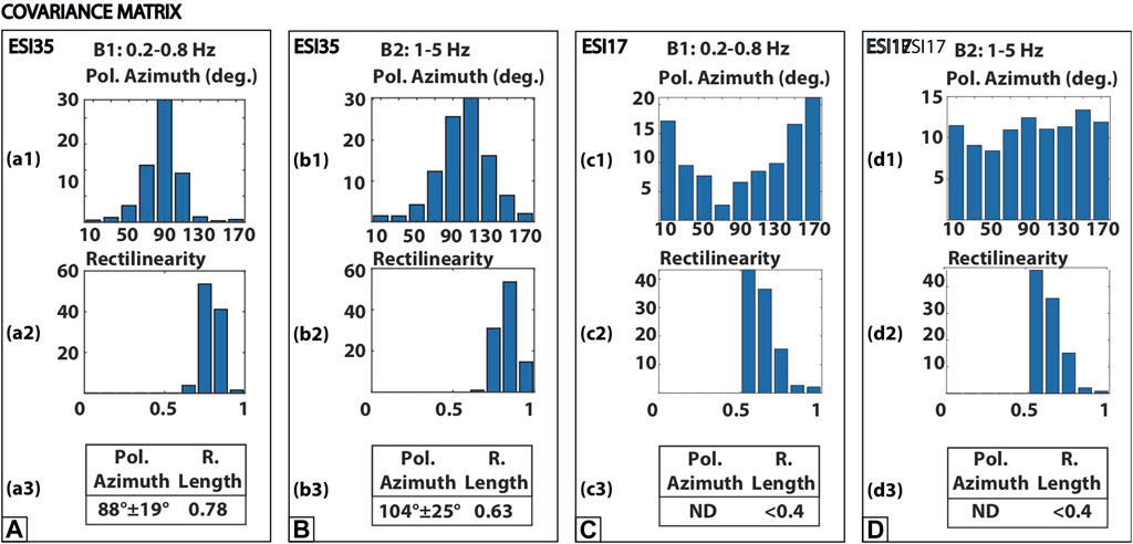
FIGURE 3. Results for ground motion polarization retrieved through the covariance matrix analysis at the two exemplificative stations ESI35 showing an effect, panels (A,B); and ESI17 not showing an effect, panels (C,D). Polarization azimuth is defined as the angle between the projection on the horizontal plane of the polarization vector and north, measured clockwise. This parameter gives a clear indication on the predominant polarization direction of horizontal ground motion (0° corresponds to geographic North; 90° and 180° correspond to geographic East and South, respectively). Histograms of polarization azimuth values are obtained in the frequency band 0.2–0.8 Hz (panels a1 and c1) and in the frequency band 1–5 Hz (panels b1 and d1). Similarly, in panels a2, b2, c2, and d2, we also add histograms of the rectilinearity values, given by Eq. 4. This parameter ranges between 0 (pure spherical motion) and 1 (pure rectilinear motion). Finally, in panels a3, b3, c3, and d3, we add final resulting parameters of the covariance matrix analysis: polarization azimuth and RL, the latter representing the concentration/spread of polarization azimuth distribution (Eq. 6).
In the Supplementary Material, we add results at the other recording stations, using a similar representation.
The time–frequency (TF) polarization analysis was proposed by Vidale (1986) and was subsequently used by Burjánek et al. (2012). This technique can provide robust results, overcoming the bias that could be introduced by the denominator spectrum in the HVSR calculation. The continuous wavelet transform (CWT, Kulesh et al., 2007) is applied to signals in order to select time windows whose length matches the dominant period: it affects all the polarization parameters and the analysis resolution. Signals are thus decomposed in the time–frequency domain, and the polarization analysis is applied. For each time–frequency pair, polarization is characterized by an ellipsoid from which the polarization azimuth is defined as the azimuth of the major axis projected to the horizontal plane from North.
In Figure 4, we show results obtained at stations ESI35 and ESI17. In panels a1 and b1, we plot the ellipticity versus frequency which is defined, according to Vidale (1986), as the ratio between the length of the minor and major axes: ellipticity approaches 0 when ground motion is linearly polarized. Unfortunately, in this dataset, we found that this parameter is not sensitive enough to distinguish linearly polarized motion. In fact, we obtained similar values at ESI35 and ESI17, while both the HVSR and covariance matrix techniques highlighted the occurrence of directional amplification at ESI35 and the absence of effects at ESI17. Therefore, it is hard to find a semi-quantitative criterion to interpret the polarization strength using ellipticity; thus, we use this technique only to validate results obtained through the HVSR and covariance matrix techniques in terms of polarization azimuth. Azimuth values obtained from all over the time series are cumulated and plotted in panels a2 and b2 and represented using polar plots. The contour scale represents the relative frequency of occurrence of each value; the distance to the center represents the signal frequency in Hz (panels a2 and b2); and white dotted circles indicate frequencies of 1 Hz, 3 Hz, and 8 Hz. The mean polarization azimuth and standard deviation are calculated at stations where the HVSR analysis highlighted the occurrence of directional amplification, at the frequency F0, as identified by the HVSR technique. At station ESI35, we obtained values of 83°±14° and 114°±22°, considering HVSR peak frequencies of 0.6 and 1.9, respectively. At station ESI17, such parameters were not defined since the HVSR technique did not reveal any directional amplification effects.
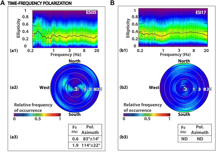
FIGURE 4. Results for time–frequency polarization analysis at stations ESI35 (A) and ESI17 (B). In panels a1 and b1, we show ellipticity versus frequency. It is defined as the ratio between the length of the minor and major axes and approaches 0 when ground motion is linearly polarized. In panels a2 and b2, polarization azimuth values obtained from all over the time series analyzed are cumulated and graphed using polar plots where the contour scale represents the relative frequency of occurrence of each value, and the distance to the center represents the signal frequency in Hz. Dashed circles depict frequencies of 1 Hz, 3 Hz, and 8 Hz. Finally, in panels a3 and b3, a summary of obtained results is shown.
In the Supplementary Material, we furnish the results at all stations.
In previous sections, we described the three methodologies and the analysis flow (Section 3) that we applied to investigate ground motion directional amplification and polarization. Their combined use furnished redundant results and led to a robust estimate of the observed effect overcoming limitations intrinsic to each of them. In the Supplementary Table S2, we report analysis results for the three techniques for the two frequency bands. They include the estimation of the following parameters:
- Directional amplification through HVSR calculation: F0, AMAX, polarization azimuth AZ (not associated standard deviation, see Section 3.1) and directionality index (DI). The common condition for amplification effects is AMAX>2 (according to SESAME 2004 guidelines). We, therefore, did not further analyze stations with HVSR not exceeding this threshold (indicated in Supplementary Table S2 as “no peaks”). Furthermore, we chose the condition for directional HVSR as DI > 1.4. When this condition was not satisfied, the parameter AZ was not estimated (indicated as “ND” in Supplementary Table S2).
- Covariance matrix analysis in the time domain after bandpass filtering signals in two frequency ranges, 0.2–0.8 Hz and 1–5 Hz: Polarization azimuth AZ (with associated standard deviation) and resultant length RL (Section 3.2). The condition for polarized ground motion is given by RL >0.4, and when not satisfied, the parameter AZ was not estimated (indicated as “ND” in Supplementary Table S2).
- Time–frequency analysis: Polarization azimuth AZ and standard deviation (Section 3.3) were evaluated in the frequency equal to F0 when DI>1.4 (otherwise indicated as “ND” in Supplementary Table S2).
At first, we investigate the consistency of results obtained from HVSR and covariance matrix analysis, in terms of the polarization strength (by comparing parameters DI and RL) and in terms of polarization azimuth values. In the frequency band 0.2–0.8 Hz, seven stations do not show any amplification effects; at seven stations, the results from the two techniques are not consistent (identified in Supplementary Table S2 in red as “discrepant res”); at 47 stations, the two techniques consistently highlight the occurrence of directional amplification and polarization effects; at 14 stations, the two techniques furnish consistent results but no directional effects (Supplementary Table S2). In the frequency band 1–5 Hz, 26 stations do not show any amplification effects; at eight stations, the results by the two techniques are not consistent (identified in Supplementary Table S2 in red as “discrepant res”); at 31 stations, the two techniques consistently highlight the occurrence of directional amplification and polarization effects; at 10 stations, the two techniques furnish consistent results but no directional effects (Supplementary Table S2).
Second, we compare polarization azimuth values obtained from the three techniques considering the two frequency bands, 0.2–0.8 Hz and 1–5 Hz (Supplementary Figure S13). We found that such values at all stations differ by less than 30°, which is an acceptable approximation range even considering that during the sensor placement in the ground, errors in the order of 10°–15° may frequently happen when manually aligning to geographic north. Therefore, in Supplementary Table S2, we give the final effect in terms of the geographical direction evaluated as a mean of azimuth values and in terms of the frequency band (from the HVSR analysis).
In Figure 2 and in Supplementary Figures S1–S11, we show results at all stations. Moreover, in Supplementary Figure S12, we add some examples for inconsistent results, suggesting that such discrepancies are related to the strict constraints that we use to distinguish between directional/non-directional and polarized/non-polarized motion.
In Figure 5, we summarize the results gathered by the covariance matrix analysis performed bandpass filtering in the two frequency bands, 0.2–0.8 Hz (top panel) and 1–5 Hz (bottom panel). Due to the high station density in Casamicciola village, on the left-bottom side of each panel, an inset is produced and focused on this area. In addition, we also add the mapped fault systems in the investigated area (Figure 1). Red triangles indicate stations at which the applied techniques consistently highlight the occurrence of directional amplification and polarization effects (Section 3.1), and polarization azimuth distribution is plotted as a rose diagram. The other stations not showing a directional effect are depicted using yellow triangles. In Figure 5, we also produce maps of the resultant length RL by using an inverse distance squared interpolation. In such contour plots, red colors correspond to linearly polarized motion, while blue colors correspond to non-polarized motion.
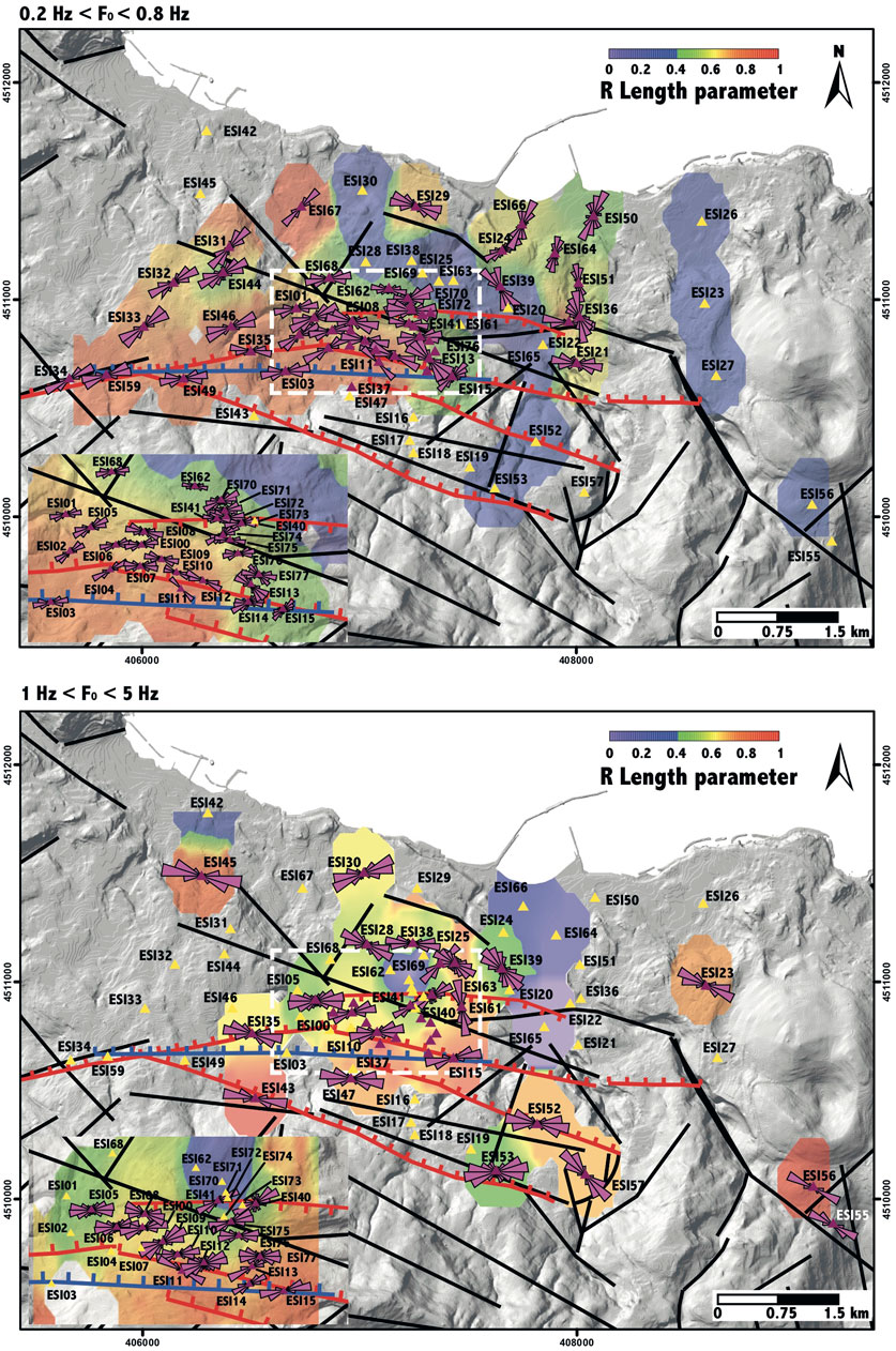
FIGURE 5. Results obtained in the two frequency bands, 0.2–0.8 Hz (top panel) and 1–5 Hz (bottom panel), through the covariance matrix analysis. The inset in the left-bottom is focused on Casamicciola village. Faults in the area are reported (red lines), as is the causative fault of the 2017 earthquake (blue line). Stations with directional amplification and polarization effects are depicted through red triangles, and the others, with yellow triangles. Polarization azimuth distribution is plotted as a rose diagram. Contour maps of the resultant length are produced using an inverse distance squared interpolation (red colors correspond to linearly polarized motion).
There are several stations arranged along two N–S trending strips, showing non-directional amplification effects (ESI19, 20, 22, 23, 25, 26, 27, 28, 30, 38, 52, 53, 61, and 63). In the northwestern sector of the studied area (Fango and Lacco Ameno villages, see Figure 1), stations show polarized motion, with high values of the RL parameter and polarization azimuth tending to be oriented in the NE–SW direction (stations ESI31, 32, 33, 44, and 67). Such observations agree with those of Martino et al. (2020), who found ground motion polarization mostly in the NE–SW direction on Zaro promontory, one km from our stations and along a fault system trending NW–SE. This polarization effect at a high angle to the fault strike could be ascribed to stiffness anisotropy caused by fracture rocks associated with fault damage zones (Pischiutta et al., 2017). The high-angle effects of the fault strike are also evident in the NE sector of the investigated area and close to the coast, with polarization tending to be oriented in the NNE–SSE direction (stations ESI36, 50, 51 64, and 66), nearly orthogonal to ESE–WSW faults). In both areas, polarization at a high angle to the fault strike is observed only in the frequency band 0.2–0.8 Hz, while they are absent in the frequency band 1–5 Hz, suggesting that such effects are produced by heterogeneities at deeper depth (hundreds of meters considering shear wave values in the order of 300–600 m/s).
However, when approaching the active normal fault (red lines in Figures 1, 3), polarization tends to be fault-parallel, even following fault strike oscillation from ENE–WSW to EW. This is also in agreement with the coseismic ruptures (yellow lines in Figures 1, 3) and causative fault of the 2017 earthquake (blue lines in Figures 1, 3). This effect is evident in both frequency bands (0.1–0.8 Hz and 1–5 Hz) and, due to the high number of installed stations, it is particularly clear in the sector of Casamicciola village that suffered the highest damage (X MCS) during the last earthquake (see the inset in the bottom panel).
In the lack of further constraints, we propose the following two hypothetical explanations for this parallel relation between ground motion polarization and the strike of these active system faults.
1) The active fault structure may act as a waveguide. Polarization parallel to the fault strike has been widely observed both in active (Lewis et al., 2005; Spudich & Olsen, 2001, and references therein) and inactive faults (Rovelli et al., 2002), where damaged rocks with high crack density produce low-velocity fault zone layers (Ben-Zion & Sammis 2003, and references therein) which act as a waveguide trapping seismic energy as a result of constructive interference of critically reflected phases (Ben-Zion and Aki 1990; Li & Leary 1990; Li et al., 1997).
2) Along the active fault system of the study area, most of the fluids rise from the deep to the superficial water (Di Napoli et al., 2009, and references therein). Crampin and Zatsepin (1997) observed that in the presence of fluid-saturated fractures, a 90°-flip occurs in the seismic anisotropy fast direction, and the anisotropy fast direction becomes orthogonal to cracks. This effect was related to pore pressure variation causing the reorganization of open and closed fluid-filled microcracks (Crampin et al., 2002; Crampin et al., 2004; Padhy & Crampin, 2006; Pastori et al., 2019). Moreover, a 90° flip was observed also by Bonness and Zoback, (2006) who ascribed this effect to structural anisotropy. Pischiutta et al. (2014 and 2015) and Panzera et al. (2017) found that in fault damage zones, ground motion polarization and velocity anisotropy show an orthogonal relation. Therefore, in the area hit by the 2017 earthquake, the presence of recently formed faults and coseismic ruptures affected by relevant hydrothermal fluid circulation (Di Napoli et al., 2009; Falanga et al., 2021) may cause a 90° flip of both ground motion polarization (which, thus, becomes parallel to fracture) and seismic anisotropy fast direction (which, thus, may become orthogonal to fractures). However, further analyses are needed to test this latter hypothesis, implying a study of seismic anisotropy to confirm the occurrence of a 90° flip. Unfortunately, during their short operating periods, our stations did not record any seismic events. Moreover, up to now, earthquake recordings at stations of the temporary network installed by INGV to detect aftershocks are poor and not appropriate for anisotropy studies.
A final consideration regards the possibility that observed amplification may be due to the Mt. Epomeo topography, such as due to constructive interference of seismic waves diffracted by the convex shape of topography, according to the “topo resonant model” (Burjanek et al., 2014a; Burjanek et al., 2014b), where the resonance frequency is related to the hill dimension and the mean shear-wave velocity (Géli et al., 1988). We exclude the role of Mt. Epomeo topography since the effect is clearly concentrated close to the causative fault of the 2017 earthquake, particularly in the frequency band 0.2–0.8 Hz. Moreover, amplification due to topography convexity is expected on the top, while here, stations showing amplification are mainly located at the lower slope of Mt. Epomeo, and stations installed at the middle slope do not show any effects (e.g., ESI16, ESI17, ESI18, ESI19, and ESI47).
These findings also confirm those of several recent papers highlighting that on topography, rather than the sole convex shape, other features in the subsoil can have a prevailing role in producing directional effects, such as impedance contrasts (Baron et al., 2021), large-scale open cracks (Moore et al., 2011; Burjánek et al., 2012), or microcracks in fractured rocks associated with fault activity (Martino et al., 2006; Marzorati et al., 2011; Pischiutta et al., 2017).
- We determined polarization and directional amplification patterns in northern Ischia, across active fault systems responsible for the 2017 Md 4.0 earthquake, considering both the main and secondary amplification peaks.
- Our observations suggest that horizontal polarization patterns depend on the site and are mainly controlled by the local geology, as suggested by several other studies on fault zones (Marzorati et al., 2011), volcanoes (Falsaperla et al., 2010; Cusano et al., 2020a; Cusano et al., 2020b), and landslides (Burjanek et al., 2010).
- On older faults and geomorphological lineaments, we found polarization at a high angle to the fault strike, consistent with several studies (Panzera et al., 2014).
- Conversely, across the active fault system, polarization becomes fault-parallel, suggesting a strong correlation with coseismic ruptures and active faults. This can be interpreted in terms of fault-guided waves, and/or furthermore, a role is probably played by the intense fluid circulation in the hydrothermal system, causing the 90° flip of polarization (and seismic anisotropy). Therefore, in this latter interpretation, time variations of ground motion polarization may be further investigated for seismic and geochemical monitoring because they can indicate some variations in the hydrothermal system (as fluid flow increase/decrease), as in Petrosino and De Siena, (2021).
The data analyzed in this study are subject to the following licenses/restrictions: Raw data (ambient noise recordings) for this research are still not publicly available because of another paper still in preparation by the INGV EMERSITO task force; the preliminary results are being shown at international meetings (Vassallo et al., 2018a; Vassallo et al., 2018b). Therefore, the access is currently restricted to the INGV EMERSITO task force, but the embargo will be released in the following months. We have begun archiving metadata in an appropriate repository, but the process is not complete. They include data files representing the polarization results and results of HVSR analysis. Software directional amplification was investigated by using the open source software “Geopsy” available at https://www.geopsy.org. Software for polarization analysis is available in this in-text data citation references: Petrosino and De Siena, (2021), at the Open Science Framework, link: osf.io/kqtbp. . Requests to access these datasets should be directed to emersito@ingv.it.
MP and SP contributed in the field by collecting seismic noise data. MP analyzed data to assess directional amplification and time–frequency polarization. SP analyzed data to assess ground motion polarization through the covariance matrix analysis. RN provided comparison with geological and structural data that she collected in other previous published works. MP wrote the manuscript draft and produced Figure 2 and the Supplementary Material. RN produced Figure 1, and SP realized Figure 3. All authors contributed to the manuscript writing and in result interpretation.
The authors are grateful to the INGV EMERSITO task force, which carried out data acquisition in the field after the 2017 Casamicciola earthquake. Part of this work has been developed in the framework of the INGV research project POLARTIME: POLARization analyses To Image crustal structure and fluid Migration Episodes at Ischia island (Ricerca Libera 2021).
The authors declare that the research was conducted in the absence of any commercial or financial relationships that could be construed as a potential conflict of interest.
All claims expressed in this article are solely those of the authors and do not necessarily represent those of their affiliated organizations, or those of the publisher, the editors, and the reviewers. Any product that may be evaluated in this article, or claim that may be made by its manufacturer, is not guaranteed or endorsed by the publisher.
The Supplementary Material for this article can be found online at: https://www.frontiersin.org/articles/10.3389/feart.2022.999222/full#supplementary-material
Acocella, V., and Funiciello, R. (1999). The interaction between regional and local tectonics during resurgent doming: The case of the island of Ischia, Italy. J. Volcanol. Geotherm. Res. 88, 109–123. doi:10.1016/s0377-0273(98)00109-7
Alessio, G., Esposito, E., Ferranti, L., Mastrolorenzo, G., and Porfido, S. (1999). Correlazione tra sismicità ed elementi strutturali nell’isola di Ischia. Italian J. Quat. Sci. 9, 303–308.
Baron, J., Primofiore, I., Klin, P., Vessia, G., and Laurenzano, G. (2021). Investigation of topographic site effects using 3D waveform modelling: Amplification, polarization and torsional motions in the case study of arquata del tronto (Italy). Bull. Earthq. Eng. 20 (2), 677–710. doi:10.1007/s10518-021-01270-2
Ben-Zion, Y., and Aki, K. (1990). Seismic radiation from an SH line source in a laterally heterogeneous planar fault zone. Bull. seism. Soc. Am. 80, 971–994.
Ben-Zion, Y., and Sammis, C. G. (2003). Characterization of fault zones. Pure appl. Geophys. 160, 677–715.
Boness, N. L., and Zoback, M. D. (2006). Mapping stress and structurally controlled crustal shear velocity anisotropy in California. Geol. 34 (10), 825–828. doi:10.1130/g22309.1
Bruno, P. P. G., de Alteriis, G., and Florio, G. (2002). The Western undersea section of the Ischia volcanic complex (Italy, Tyrrhenian Sea) inferred by marine geophysical data. Geophys. Res. Lett. 29 (9), 57-1–57-4. doi:10.1029/2001gl013904
Burjánek, J., Edwards, B., and Fäh, D. (2014a). Empirical evidence of local seismic effects at sites with pronounced topography: A systematic approach. Geophys. J. Int. 1, 608–619. doi:10.1093/gji/ggu014
Burjánek, J., Fäh, D., Pischiutta, M., Rovelli, A., Calderoni, G., and Bard, P.-Y. (2014b). Site effects at sites with pronounced topography: Overview & recommendations. Res. Rep. E. U. Proj. NERA-JRA1 Work. group 64. doi:10.3929/ethz-a-010222426
Burjanek, J., Gassner-Stamm, G., Poggi, V., Moore, J. R., and Fah, D. (2010). Ambient vibration analysis of an unstable mountain slope. Geophys. J. Int. 180, 820–828. doi:10.1111/j.1365-246x.2009.04451.x
Burjánek, J., Kleinbrod, U., and Fah, D. (2019). Modeling the seismic response of unstable rock mass with deep compliant fractures. Journal of geophysical research: Solid Earth. J. Geophys. Res. Solid Earth 124, 13, 039–113, 059. doi:10.1029/2019jb018607
Burjánek, J., Moore, J. R., Yugsi-Molina, F. X., and Fäh, D. (2012). Instrumental evidence of normal mode rock slope vibration. Geophys. J. Int. 188, 559–569. doi:10.1111/j.1365-246x.2011.05272.x
Calderoni, G., Di Giovambattista, R., Pezzo, G., Albano, M., Atzori, S., Tolomei, C., et al. (2019). Seismic and geodetic evidences of a hydrothermal source in the Md 4.0, 2017, Ischia earthquake (Italy). J. Geophys. Res. Solid Earth 124, 5014–5029. doi:10.1029/2018jb016431
Crampin, S., Peacock, S., Gao, Y., and Chastin, S. (2004). The scatter of time-delays in shear-wave splitting above small earthquakes. Geophys. J. Int. 156 (1), 39–44. doi:10.1111/j.1365-246x.2004.02040.x
Crampin, S., Volti, T., Chastin, S., Gudmundsson, A., and Stefánsson, R. (2002). Indication of high pore-fluid pressures in a seismically-active fault zone. Geophys. J. Int. 151 (2), F1–F5. doi:10.1046/j.1365-246x.2002.01830.x
Crampin, S., and Zatsepin, S. V. (1997). Modelling the compliance of crustal rock—II. Response to temporal changes before earthquakes. Geophys. J. Int. 129 (3), 495–506. doi:10.1111/j.1365-246x.1997.tb04489.x
Cubellis, E., and Luongo, G. (1998). “Il Contesto Fisico, in AA.VV., il Terremoto del 28 luglio 1883 a Casamicciola nell’isola di Ischia. Presidenza Consiglio dei Ministri,” in Servizio sismico Nazionale (Poligrafico e Zecca dello Stato: Roma: Italy), 49–123.
Cultrera, G., Rovelli, A., Mele, G., Azzara, R., Caserta, A., and Marra, F. (2003). Azimuth dependent amplification of weak and strong ground motions within a fault zone, Nocera Umbra, Central Italy. J. Geophys. Res. 108 (B3), 2156–2170. doi:10.1029/2002jb001929
Cusano, P., Petrosino, S., De Lauro, E., and Falanga, M. (2020a). The whisper of the hydrothermal seismic noise at Ischia Island. J. Volcanol. Geotherm. Res. 389, 106693. doi:10.1016/j.jvolgeores.2019.106693
Cusano, P., Petrosino, S., De Lauro, E., De Martino, S., and Falanga, M. (2020b). Characterization of the seismic dynamical state through joint analysis of earthquakes and seismic noise: The example of Ischia volcanic island (Italy). Adv. Geosci. 52, 19–28. doi:10.5194/adgeo-52-19-2020
De Vita, S., Sansivero, F., Orsi, G., Marotta, E., and Piochi, M. (2010). Volcanological and structural evolution of the Ischia resurgent caldera (Ischia) over the past 10 ka. Geol. Soc. Am. 464, 193–239. doi:10.1130/2010.2464(10)
Del Gaudio, V., and Wasowski, J. (2007). Directivity of slope dynamic response to seismic shaking. Geophys. Res. Lett. 34, L12301. doi:10.1029/2007gl029842
Del Prete, S., and Mele, R. (2006). Il contributo delle informazioni storiche per la valutazione della propensione al dissesto nell’Isola d’Ischia (Campania). Rend. Soc. Geol. It 2, 29–47.
Del Prete, S., and Mele, R. (1999). L'Influenza dei fenomeni d'instabilita di versante nel quadro morfoevolutivo della costa dell'isola d'Ischia. Boll. della Soc. Geol. Ital. 118 (2), 339–360.
Della Seta, M., Esposito, C., Marmoni, G. M., Martino, S., Paciello, A., Perinelli, C., et al. (2015). Geological constraints for a conceptual evolutionary model of the slope deformations affecting Mt. Nuovo at Ischia (Italy). Italian J. Eng. Geol. Environ. 15 (2), 15–28. doi:10.4408/IJEGE.2015-02.O-02
Di Giulio, G., Cara, F., Rovelli, A., Lombardo, G., and Rigano, R. (2009). Evidences for strong directional resonances in intensely deformed zones of the Pernicana fault, Mount Etna, Italy. J. Geophys. Res. 114. doi:10.1029/2009JB006393
Di Giulio, G., Punzo, M., Bruno, P. P., Cara, F., and Rovelli, A. (2019). Using a vibratory source at Mt. Etna (Italy) to investigate the wavefield polarization at Pernicana Fault. Near Surf. Geophys. 17, nsg.12051–329. doi:10.1002/nsg.12051
Di Napoli, R., Aiuppa, A., Bellomo, S., Brusca, L., D'Alessandro, W., Candela, E. G., et al. (2009). A model for Ischia hydrothermal system: Evidences from the chemistry of thermal groundwaters. J. Volcanol. Geotherm. Res. 186 (3-4), 133–159. doi:10.1016/j.jvolgeores.2009.06.005
Falanga, M., Cusano, P., De Lauro, E., and Petrosino, S. (2021). Picking up the hydrothermal whisper at Ischia Island in the Covid-19 lockdown quiet. Sci. Rep. 11, 8871. doi:10.1038/s41598-021-88266-9
Falsaperla, S., Cara, F., Rovelli, A., Neri, M., Behncke, B., and Acocella, V. (2010). Effects of the 1989 fracture system in the dynamics of the upper SE flank of etna revealed by volcanic tremor data: The missing link? J. Geophys. Res. 115, B11306. doi:10.1029/2010JB007529
Hailemikael, S., Lenti, L., Martino, S., Paciello, A., Rossi, D., and Scarascia Mugnozza, G. (2016). Ground-motion amplification at the colle di Roio ridge, central Italy: A combined effect of stratigraphy and topography. Geophys. J. Int. 206, 1–18. doi:10.1093/gji/ggw120
Häusler, M., Michel, C., Burjánek, J., and Fäh, D. (2019). Fracture network imaging on rock slope instabilities using resonance mode analysis. Geophys. Res. Lett. 46, 6497–6506. doi:10.1029/2019gl083201
Jurkevics, A. (1988). Polarization analysis of three component array data. Bull. seism. Soc. Am. 78, 1725–1743.
Kanasewich, E. R. (1981). Time sequence analysis in Geophysics. Edmonton: University of Alberta Press, 477.
Konno, K., and Ohmachi, T. (1998). Ground-motion characteristics estimated from spec- tral ratio between horizontal and vertical components of microtremor. Bull. Seismol. Soc. Am. 88, 228–241. doi:10.1785/bssa0880010228
Kulesh, M., Diallo, M., Holschneider, M., Kurennaya, K., Kruger, F., Ohrnberger, M., et al. (2007). Polarization analysis in the wavelet domain based on the adaptive covariance method. Geophys. J. Int. 170, 667–678. doi:10.1111/j.1365-246x.2007.03417.x
Lewis, M. A., Peng, Z., Ben-Zion, Y., and Vernon, F. L. (2005). Shallow seismic trapping structure in the San Jacinto fault zone near Anza, California. Geophys. J. Int. 162, 867–881. doi:10.1111/j.1365-246x.2005.02684.x
Li, Y. G., and Leary, P. C. (1990). Fault zone trapped seismic waves. Bull. Seismol. Soc. Am. 80, 1245–1271. doi:10.1785/bssa0800051245
Li, Y. L., Ellsworth, G. W., Thurber, C. H., Malin, P. E., and Aki, K. (1997). Observations of fault zone trapped waves excited by explosions at the San Andreas fault, central California. Bull. seism. Soc. Am. 87, 210–221.
Martino, S., Caprari, P., Della Seta, M., Esposito, C., Fiorucci, M., Hailemikael, S., et al. (2020). Influence of geological complexities on local seismic response in the Municipality of Forio (Ischia Island, Italy). Ital. J. Eng. Geol. Environ. 2, 43–62. doi:10.4408/IJEGE.2020-02.O-04
Martino, S., Minutolo, A., Paciello, A., Rovelli, A., Scarascia Mugnozza, G., and Verrubbi, V. (2006). Evidence of amplification effects in fault zone related to rock mass jointing. Nat. Hazards (Dordr). 39, 419–449. doi:10.1007/s11069-006-0001-2
Marzorati, S., Ladina, C., Falcucci, E., Gori, S., Saroli, A., Ameri, G., et al. (2011). Site effects “on the rock”: The case of castelvecchio subequo (L’aquila, central Italy). Bull. Earthq. Eng. 9, 841–868. doi:10.1007/s10518-011-9263-5
Moore, J. R., Geimer, P. R., Finnegan, R., and Thorne, M. (2018). Use of seismic resonance measurements to determine the elastic modulus of freestanding rock masses. Rock Mech. Rock Eng. 51 (12), 3937–3944. doi:10.1007/s00603-018-1554-6
Moore, J. R., Gischig, V., Burjánek, J., and Loew, S., Fäh D. (2011). site effects in unstable rock slopes: Dynamic behavior of the randa instability (Switzerland). Bull. Seismol. Soc. Am., 101. doi:10.1785/0120110127
Moore, J. R., Gischig, V., Burjànek, J., Loew, S., and Faeh, D. (2011). Site effects in unstable rock slopes: Dynamic behavior of the randa instability (Switzerland). Bull. Seismol. Soc. Am. 101, 3110–3116. doi:10.1785/0120110127
Nakamura, Y. (1989). A method for dynamic characteristics estimation of subsurface using microtremors on the ground surface. Q. Rep. RTRI Jpn. 30, 25–33.
Nappi, R., Alessio, G., and Bellucci Sessa, E. (2010). A case study comparing landscape metrics to geologic and seismic data from the Ischia Island (southern Italy). Appl. Geomat. 2, 73–82. doi:10.1007/s12518-010-0023-z
Nappi, R., Alessio, G., Gaudiosi, G., Nave, R., Marotta, E., Siniscalchi, V., et al. (2018a). The 21 August 2017 Md 4.0 Casamicciola earthquake: First evidence of coseismic normal surface faulting at the Ischia volcanic island. Seismol. Res. Lett. 89, 1323–1334. doi:10.1785/0220180063
Nappi, R., Alessio, G., Gaudiosi, G., Nave, R., Marotta, E., Siniscalchi, V., et al. (2018b). Reply to “comment on ‘the 21 August 2017 Md 4.0 Casamicciola earthquake: First evidence of coseismic normal surface faulting at the Ischia volcanic island’ by nappiet al.(2018)” by V. De novellis, S. Carlino, R. Castaldo, A. Tramelli, C. De luca, N. A. Pino, S. Pepe, V. Convertito, I. Zinno, P. De Martino, M. Bonano, F. Giudicepietro, F. Casu, G. Macedonio, M. Manunta, M. Manzo, G. Solaro, P. Tizzani, G. Zeni, and R. Lanari. 2018 90 (1), 316–321. doi:10.1785/0220180339
Nappi, R., Porfido, S., Paganini, E., Vezzoli, L., Ferrario, M. F., Gaudiosi, G., et al. (2021). The 2017, MD = 4.0, Casamicciola earthquake: ESI-07 scale evaluation and implications for the source model. Geosciences 11, 44. doi:10.3390/geosciences11020044
Nardone, L., Vassallo, M., Sapia, V., Petrosino, S., Pischiutta, M., Di Vito, M., et al. (2022). A geophysical multidisciplinary approach to investigate the shallow subsoil structures in volcanic environment: The case of Ischia island. J. Volcanol. Geotherm. Res.
Padhy, S., and Crampin, S. (2006). High pore-fluid pressures at Bhuj, inferred from 90-flips in shear-wave polarizations. Geophys. J. Int. 164 (2), 370–376. doi:10.1111/j.1365-246x.2006.02854.x
Panzera, F., Halldorsson, B., and Vogfjörðc, K. (2017). Directional effects of tectonic fractures on ground motion site amplification from earthquake and ambient noise data: A case study in South Iceland. Soil Dyn. Earthq. Eng. 97, 143–154. doi:10.1016/j.soildyn.2017.03.024
Panzera, F., Pischiutta, M., Lombardo, G., Monaco, C., and Rovelli, A. (2014). Wavefield polarization in fault zones of the Western flank of Mt. Etna: Observations and fracture orientation modelling. Pure Appl. Geophys. 171, 3083–3097. doi:10.1007/s00024-014-0831-x
Panzera, F., Tortorici, G., Romagnoli, G., Marletta, G., and Catalano, S. (2020). Empirical evidence of orthogonal relationship between directional site effects and fracture azimuths in an active fault zone: The case of the Mt. Etna lower eastern flank. Eng. Geol. 279, 105900. doi:10.1016/j.enggeo.2020.105900
Pastori, M., Baccheschi, P., and Margheriti, L. (2019). Shear wave splitting evidence and relations with stress field and major faults from the “Amatrice-Visso-Norcia Seismic Sequence”. Tectonics 38 (9), 3351–3372. doi:10.1029/2018tc005478
Petrosino, S., Damiano, N., Cusano, P., Vito, D., de Vita, S., and Del Pezzo, E. (2012). Subsurface structure of the Solfatara volcano (Campi Flegrei caldera, Italy) as deduced from joint seismic-noise array, volcanological and morphostructural analysis. Geochem. Geophys. Geosystems 13 (7). doi:10.1029/2011GC004030
Petrosino, S., and De Siena, L. (2021). Fluid migrations and volcanic earthquakes from depolarized ambient noise. Nat. Commun. 12 (1), 6656–6658. doi:10.1038/s41467-021-26954-w
Pischiutta, M. (2010). The polarization of horizontal ground motion: An analysis of possible causes, Ph.D. thesis, Universita` di Bologna: Alma Mater Studiorum’, 172.
Pischiutta, M., Cianfarra, P., Salvini, F., Cara, F., and Vannoli, P. (2018). A systematic analysis of directional site effects at stations of the Italian seismic network to test the role of local topography,. Geophys. J. Int. 214 (1), 635–650. doi:10.1093/gji/ggy133
Pischiutta, M., Fondriest, M., Demurtas, M., Magnoni, F., Di Toro, G., and Rovelli, A. (2017). Structural control on the directional amplification of seismic noise (Campo Imperatore, central Italy). Earth Planet. Sci. Lett. 471, 10–18. doi:10.1016/j.epsl.2017.04.017
Pischiutta, M., Pastori, M., Improta, L., Salvini, F., and Rovelli, A. (2014). Orthogonal relation between wavefield polarization and fast S-wave direction in the val d’Agri region: An integrating method to investigate rock anisotropy. J. Geophys. Res. Solid Earth 119, 396–408. doi:10.1002/2013jb010077
Pischiutta, M., Salvini, F., Fletcher, J. B., Rovelli, A., and Ben-Zion, Y. (2012). Horizontal polarization of ground motion in the hayward fault zone at fremont, California: Dominant fault-high-angle polarization and fault-induced cracks. Geophys. J. Int. 188 (3), 1255–1272. doi:10.1111/j.1365-246x.2011.05319.x
Pischiutta, M., Savage, M., Holt, R., and Salvini, F. (2015). Fracture-related wavefield polarization and seismic anisotropy across the Greendale Fault. J. Geophys. Res. Solid Earth 120, 7048–7067. doi:10.1002/2014jb011560
Rigano, R., Cara, F., Lombardo, G., and Rovelli, A. (2008). Evidence for ground motion polarization on fault zones of Mount Etna volcano. J. Geophys. Res. 113, B10306. doi:10.1029/2007jb005574
Rovelli, A., Caserta, A., Marra, F., and Ruggiero, V. (2002). Can seismic waves be trapped inside an inactive fault zone? The case study of nocera Umbra, central Italy. Bull. Seism. Bull. Seismol. Soc. Am. 92, 2217–2232. doi:10.1785/0120010288
Sbrana, A., Marianelli, P., and Pasquini, G. (2018). Volcanology of Ischia (Italy). J. Maps 14, 494–503. doi:10.1080/17445647.2018.1498811
Sepe, V., Atzori, S., and Ventura, G. (2007). Subsidence due to crack closure and depressurization of hydrothermal systems: A case study from Mt. Epomeo (Ischia island, Italy). Terra nova. 19, 127–132. doi:10.1111/j.1365-3121.2006.00727.x
SESAME (2004). Guidelines for the implementation of the H/V spectral ratio tech- nique on ambient vibrations: Measurements, processing and interpretation. SESAME (Site Effects Assessment Using Ambient Excitations, EC-RGD, Project No. EVG1-CT-2000–00026 SESAME), European Research Project WP12, deliverable D23.12, Available at: http://sesame-fp5.obs.ujfgrenoble.fr/Deliverables 2004.
Spudich, P., Hellweg, M., and Lee, W. H. K. (1996). Directional topographic site response at Tarzana observed in aftershocks of the 1994 Northridge, California, earthquake: Implications for mainshock motions. Bull. Seismol. Soc. Am. 86 (1B), S193–S208. doi:10.1785/bssa08601bs193
Spudich, P., and Olsen, K. B. (2001). Fault zone amplified waves as a possible seismic hazard along the Calaveras Fault in central California. Geophys. Res. Lett. 28 (13), 2533–2536. doi:10.1029/2000gl011902
Tibaldi, A., and Vezzoli, L. (2004). A new type of volcano flank failure: The resurgent caldera sector collapse, Ischia, Italy. Geophys. Res. Lett. 31, L14605. doi:10.1029/2004GL020419
Tibaldi, A., and Vezzoli, L. (1998). The space problem of caldera resurgence: An example from Ischia island, Italy. Geol. Rundsch. 87, 53–66. doi:10.1007/s005310050189
Vassallo, M., Galluzzo, D., Sapia, V., Nardone, L., Pischiutta, M., and Petrosino, S. (2018a). “Site effect studies following the 2017 Mw 3.9 Ischia earthquake: The Emersito++ task force activities,” in EGU General Assembly Conference Abstracts (EGU2018-16452-1), 16452.
Vassallo, M., Galluzzo, D., Sapia, V., Nardone, L., Pischiutta, M., Petrosino, S., et al. (2018b). “Seismological and geophysical studies for site effect characterization following the 2017 Mw 3.9 Ischia earthquake,” in Millennia of Stratification between Human Life and Volcanoes: Strategies for Coexistence,Abstracts Volume of the International Meeting “Cities on Volcanoes 10”, Napoli, Italy, 2-7September 2018, 565. Miscellanea INGV N.43.
Vezzoli, L. (1998). “Island of Ischia,” in Quaderni della Ricerca scientifica. Editor L. Vezzoli (Consiglio Nazionale delle Ricerche: Roma: Italy), 1–122.
Vidale, J. E. (1986). Complex polarization analysis of particle motion. Bull. Seism. Soc. Am. 76, 1393–1405.
Vignaroli, G., Giallini, S., Polpetta, F., Sirianni, P., Gaudiosi, I., Simionato, M., et al. (2019). Domains of seismic noise response in faulted limestone (central apennines, Italy): Insights into fault-related site effects and seismic hazard. Bull. Eng. Geol. Environ. 78, 2749–2768. doi:10.1007/s10064-018-1276-8
Keywords: site amplification effects, directional amplification, ground motion polarization, Casamicciola earthquake, fault damage zone, coseismic ruptures
Citation: Pischiutta M, Petrosino S and Nappi R (2022) Directional amplification and ground motion polarization in Casamicciola area (Ischia volcanic island) after the 21 August 2017 Md 4.0 earthquake. Front. Earth Sci. 10:999222. doi: 10.3389/feart.2022.999222
Received: 12 August 2022; Accepted: 11 November 2022;
Published: 12 December 2022.
Edited by:
Mourad Bezzeghoud, Universidade de Évora, PortugalReviewed by:
Yosuke Aoki, The University of Tokyo, JapanCopyright © 2022 Pischiutta, Petrosino and Nappi. This is an open-access article distributed under the terms of the Creative Commons Attribution License (CC BY). The use, distribution or reproduction in other forums is permitted, provided the original author(s) and the copyright owner(s) are credited and that the original publication in this journal is cited, in accordance with accepted academic practice. No use, distribution or reproduction is permitted which does not comply with these terms.
*Correspondence: M. Pischiutta, bWFydGEucGlzY2hpdXR0YUBpbmd2Lml0
Disclaimer: All claims expressed in this article are solely those of the authors and do not necessarily represent those of their affiliated organizations, or those of the publisher, the editors and the reviewers. Any product that may be evaluated in this article or claim that may be made by its manufacturer is not guaranteed or endorsed by the publisher.
Research integrity at Frontiers
Learn more about the work of our research integrity team to safeguard the quality of each article we publish.