Least-squares reverse time migration based on the viscoacoustic VTI pure qP-wave equation

With the deepening of oil and gas exploration and the increasing complexity of exploration targets, the influence of anisotropy and anelasticity of subsurface media on seismic imaging cannot be ignored. The least-squares reverse time migration is developed on the idea of linear inversion, which can effectively solve the amplitude imbalance, low resolution, and serious imaging noise problems of RTM. In this paper, based on the viscoacoustic pure qP-wave equation, the corresponding demigration operator, adjoint operator, and gradient-sensitive kernel are derived, and the least-square reverse time migration imaging algorithm of viscoacoustic pure qP-wave in VTI medium is proposed. During iterative inversion, the inverse of Hessian is approximately solved to achieve stable attenuation compensation. Finally, we verify the effectiveness and applicability of the proposed viscoacoustic VTI least-squares reverse time migration imaging algorithm through the model tests and field data. The numerical results show that the method can compensate for the amplitude loss and phase distortion caused by attenuation, and correct the anisotropy-induced misalignment of the reflection interfaces, which improves the accuracy and resolution of the imaging profile.

Introduction

Numerous theories and experiments have demonstrated the prevalence of seismic anelasticity and anisotropy in subsurface media (Thomsen, 1986; Robertsson et al., 1994). The inherent anelasticity of subsurface rock layers attenuates seismic wave, causing energy loss and phase distortion (White, 1975; Dvorkin and Mavko, 2006), which impacts the quality of seismic images. Meanwhile, the anisotropy of the subsurface medium caused by mineral particle arrangement in subsurface rocks, fracture direction, or thin layer development, provokes the wave velocity to vary with the propagation direction when seismic wave propagates in the subsurface rocks (Xu et al., 2020; He et al., 2021), and this kinematic property different from that of isotropic medium affects the traveltime information of seismic wave. Ignoring anisotropy might result in non-negligible inaccuracies when researching the seismic wave propagation characteristics in real Earth media and the imaging position of structures in migration profiles. Therefore, the effects of subsurface medium anisotropy and anelasticity in seismic data processing can no longer be disregarded as requirements for seismic data resolution and image quality improvement (Wu, 2006; Sun and Zhu, 2018; Fathalian et al., 2021).

Despite the difficulties of acquiring elastic wave seismic data, the complexity of waveform separation, and the enormous computational costs, the anisotropic acoustic wave equation under the acoustic approximation (Alkhalifah, 1998) is still widely used in seismic exploration (Zhang et al., 2011). In seismic wave numerical simulation and imaging in complex VTI media, the existence of qSV-wave can lead to numerical instability, and in addition, the qSV-wave artifacts need other processing methods to eliminate (Xu et al., 2020). To avoid the interference of qSV-wave artifacts, Liu et al. (2009) propose a directly decoupled pure qP-wave equation to solve the instability existing in the conventional coupled pseudo-acoustic wave equation. Du et al. (2007) and Chu et al. (2011) obtain an approximate pure qP-wave equation in TI media that can be solved using the finite-difference method (FDM) or pseudo-spectral method (PSM). Cheng et al. (2013) derive the qP-wave pseudo-pure mode equation which is applicable to arbitrary anisotropic media and used the polarization vector to separate the P- and S-wave to further reduce the computational costs and suppress the qSV-wave artifacts. Xu and Zhou (2014) propose the pure qP-wave equation in VTI media based on the acoustic approximation (Alkhalifah, 1998), which decouples the qP- and qS-wave using the pseudo-difference operator. According to the departure between the direction of the wave vector and SV-wave vibration, Cheng and Kang, (2016) extract the scalar pure qP-wave field from the coupled wavefield to improve the imaging accuracy. Li and Zhu (2018) derive the TTI pure qP-wave equation containing Poisson’s equation, which can be solved by the FDM.

In addition to research on anisotropy, scholars have made many studies and efforts in seismic wave propagation and imaging in anelasticity media. To compensate for the energy attenuation in seismic data, inverse Q filtering is developed (Bickel and Natarajan, 1985; Hargreaves and Calvert, 1991; Li and Wang, 2007). However, the theoretical basis of inverse Q filtering is wave propagation in a one-dimensional subsurface medium model, which is not applicable to inhomogeneous complex geological conditions (Zhang et al., 2010). Based on the continuous development of ray theory, one-way wave equation, and two-way wave equation methods, more accurate inverse Q migration algorithms are gradually developed in the field of prestack depth migration. The ray theory-based attenuation compensation migration method is difficult to solve the problem of multipath and caustics area of seismic wave, and therefore it is difficult to provide high-quality imaging results under complex geological conditions (Xie et al., 2009). Based on the one-way wave equation theory, Mittet et al. (1995) propose an attenuation compensation strategy, which is later applied to different wavefield extension operators by scholars (Wang, 2008; Valenciano et al., 2011). However, the one-way wave equation migration cannot effectively image steeply inclined reflection interfaces, which limits its application in complex geological regions. In contrast, the two-way wave equation reverse time migration (RTM) imaging method (Baysal et al., 1983; McMechan, 1983) is one of the most accurate imaging techniques which can handle all wave types, without angular constraints, and can handle velocity drastic variations. In recent years, Q-compensated RTM algorithms have been more widely studied and applied. In the RTM process, the way to compensate for the Q absorption attenuation effect is to make the seismic wave energy increase during the wavefield propagation (Zhu et al., 2014; Guo et al., 2016). During the backward propagation of the viscoacoustic seismic wavefield, the rapid growth of high-frequency components energy can lead to instability of the numerical results. To solve this problem, scholars have proposed methods such as adding regularization terms (Zhang et al., 2010; Tian et al., 2015; Zhao et al., 2018), and low-pass filtering (Bai et al., 2013; Zhu et al., 2014). However, none of these methods can fundamentally solve the instability problem.

To further improve the accuracy of Q-compensated imaging, scholars have developed the least-squares reverse time migration (LSRTM) for anelasticity media based on the inversion idea. LSRTM treats seismic migration as an inverse problem, which can suppress imaging noise using multiple iterations, while can eliminate the negative effects of wavelet band defects to some extent and improve imaging resolution (Nemeth et al., 1999; Gu et al., 2018). LSRTM in anelasticity media can be divided into two categories: one is to keep the wavefield attenuated without changing the sign of the amplitude attenuation term, and to achieve attenuation compensation through the inverse of the Hessian matrix. Dutta and Schuster (2014) propose a Q-compensated LSRTM by approximating the inverse of Hessian to avoid the instability problem of wavefield backward propagation. Guo et al. (2017) develop an adjoint pseudo-differential scale Q-compensated imaging method to achieve amplitude compensation and phase correction by approximating the inverse Hessian matrix. Chen et al. (2017) propose to approximate the inverse of Hessian using a viscoacoustic deblurring filter and use it as a precondition to construct the Q-compensated LSRTM. Chai et al. (2017) use the Born operator for forward propagation, and use the adjoint operator to carry out the backward propagation of the residual wavefield to achieve stable compensation, so as to realize the Q-compensation LSRTM without changing the symbol of the attenuation operator. Chen et al. (2020) establish the LSRTM based on the constant fractional-order viscoacoustic wave equation. Through the inversion idea, the predicted data are matched with the observed data to obtain accurate underground reflection coefficient information and avoid the instability caused by the exponential growth of wavefield energy. This kind of method needs to solve the inverse of the Hessian matrix approximately, requiring great computation costs and computer memory, but can avoid the instability problem caused by compensation naturally. The other one is to compensate the energy loss by reversing the sign of amplitude attenuation term in the process of wavefield backward propagation. Sun et al. (2016) develop a viscoacoustic LSRTM method based on the low-rank algorithm and use the Q-compensation strategy proposed by Zhu et al. (2014) to accelerate convergence. Wang and Ba (2018) derive a viscoacoustic wave equation based on the exact dispersion relation for standard linear solids (SLSs) and construct an LSRTM algorithm while adding a regularization term to maintain the stability of the compensation process. Qu et al. (2021) develop a Q-compensated LSRTM based on the first-order viscoacoustic pseudo-differential equation and achieve stable attenuation compensation by adding a regularization term. Such methods require additional means to address the instability caused by attenuation compensation.

In order to effectively improve the quality of seismic images in anisotropic attenuated media and achieve stable attenuation compensated imaging, an LSRTM method based on the viscoacoustic VTI pure qP-wave equation is proposed in this paper. Firstly, based on the viscoacoustic VTI pure qP-wave equation, the linear representation of the viscoacoustic VTI wave equation is given according to Born approximation theory, and the corresponding demigration operator of the LSRTM is given. Finally, the imaging results demonstrate the validity and feasibility of the proposed LSRTM imaging method in viscoacoustic VTI media and show that the method can effectively improve the imaging quality in anisotropic attenuated media.

Viscoacoustic VTI pure qP-wave least-squares reverse time migration

Demigration equation of viscoacoustic VTI least-squares reverse time migration

Based on the nearly constant Q model, the two-dimensional viscoacoustic VTI pure qP-wave equation can be expressed as (Zhang et al., 2022):

$\frac{{\partial }^{2}u\left(\mathit{x},t\right)}{\partial t^2}=V^2\left(\mathit{x}\right)S\left[\eta {\left(-\mathrm{\Delta }\right)}^{\gamma +1}+\psi \frac{\partial }{\partial t}{\left(-\mathrm{\Delta }\right)}^{\gamma +0.5}\right]u\left(x,t\right)(1)$

where

$\begin{array}{l}\eta =-v^{2\gamma }\left(x\right){\omega }_0^{-2\gamma }\cos \left(\pi \gamma \right)\\ \psi =-v^{2\gamma -1}\left(x\right){\omega }_0^{-2\gamma }\sin \left(\pi \gamma \right)\end{array}(2)$

and the operator $S$ is written as:

$S=\frac{1}{2}\left(1+2\mathrm{\epsilon }{n}_x^2+\sqrt{{\left(1+2\mathrm{\epsilon }{n}_x^2\right)}^2-8\left(\mathrm{\epsilon }-\delta \right)n_z^2{n}_x^2}\right)(3)$

where $u\left(x,t\right)$ denotes seismic wavefield, $x=\left(x,z\right)$ is spatial position, $t$ denotes time; $\mathrm{\Delta }={\partial }^2/\partial z^2+\left(1+2\mathrm{\epsilon }\right){\partial }^2/\partial x^2$ defined as the pseudo-Laplacian operator in VTI medium, $\mathrm{\epsilon }$ and $\delta$denote Thomsen (1986) anisotropic parameters, $\left(n_x,n_z\right)=\overrightarrow{k}/\left|\overrightarrow{k}\right|$ denotes wave propagation direction unit vector; $\gamma =\arctan \left(1/Q\right)/\pi$ is a dimensionless parameter; Q is the quality factor; $V\left(x\right)=v\left(x\right)\cos \left(\pi \gamma /2\right)$, and $v\left(x\right)$ denotes the phase velocity at the reference frequency ${\omega }_0$. The right hand of Eq. 1 contains two fractional Laplacian operators to describe the propagation of the seismic wave in VTI anelasticity media, where the first term describes the phase dispersion, and the second term describes the energy attenuation.

In this paper, we assume that the perturbation of the seismic wavefield is mainly caused by velocity perturbation. Based on the Born approximation theory, the phase velocity $v\left(x\right)$ at reference frequency ${\omega }_0$ is the superposition of background velocity $v_0\left(x\right)$ and perturbated velocity $\delta v\left(x\right)$:

$v\left(x\right)=v_0\left(x\right)+\delta v\left(x\right)(4)$

According to the superposition principle of seismic wavefield, the perturbation of velocity field will cause the disturbance of seismic wavefield. Then the seismic wavefield $u\left(x,t\right)$ based on the velocity model $v\left(x\right)$ will be composed of background wavefield $u_0\left(x,t\right)$ and perturbated wavefield $\delta u\left(x,t\right)$, which is expressed as:

$u\left(\mathit{x},t\right)=u_0\left(x,t\right)+\delta u\left(x,t\right)(5)$

The background wavefield $u_0\left(x,t\right)$ generated in the background velocity field $v_0\left(x\right)$ satisfies the following equation:

$\frac{1}{V_0^2\left(\mathit{x}\right)}\frac{{\partial }^2{u}_0\left(\mathit{x},t\right)}{\partial t^2}=S\left[{\eta }_0{\left(-\mathrm{\Delta }\right)}^{\gamma +1}+{\psi }_0\frac{\partial }{\partial t}{\left(-\mathrm{\Delta }\right)}^{\gamma +0.5}\right]u_0\left(x,t\right)(6)$

where $V_0\left(x\right)=v_0\left(x\right)\cos \left(\pi \gamma /2\right)$, ${\eta }_0=-v_0^{2\gamma }{\omega }_0^{-2\gamma }\cos \left(\pi \gamma \right)$, ${\psi }_0=-v_0^{2\gamma -1}{\omega }_0^{-2\gamma }\sin \left(\pi \gamma \right)$.

Here we define the reflectivity model as:

$m\left(x\right)=\frac{2\delta v\left(\mathit{x}\right)}{v_0\left(\mathit{x}\right)}(7)$

To obtain the perturbated wavefield, based on Taylor expansion, there are the approximations:

$\begin{array}{l}\frac{1}{v}=\frac{1}{v_0+\delta v}\approx \frac{1}{v_0}-\frac{\delta v}{v_0^2}\\ \frac{1}{v^2}=\frac{1}{{\left(v_0+\delta v\right)}^2}\approx \frac{1}{v_0^2}-\frac{2\delta v}{v_0^3}\end{array}(8)$

Substituting Eq. 8 into Eq. 6, combined with Eq. 1, applying the first-order Born approximation, and ignoring the high-order terms at the right end of the equation, we can obtain the demigration equation (Born equation) corresponding to the viscoacoustic VTI pure qP-wave equation:

$\frac{1}{V_0^2\left(\mathit{x}\right)}\frac{{\partial }^2\delta u\left(\mathit{x},t\right)}{\partial t^2}=S\left[{\eta }_0{\left(-\mathrm{\Delta }\right)}^{\gamma +1}+{\psi }_0\frac{\partial }{\partial t}{\left(-\mathrm{\Delta }\right)}^{\gamma +0.5}\right]\delta u\left(x,t\right)+F(9)$

where $F$ is the virtual source term of the demigration equation, which is expressed as:

$F=\frac{m\left(\mathit{x}\right)}{V_0^2\left(\mathit{x}\right)}\frac{{\partial }^2{u}_0\left(\mathit{x},t\right)}{\partial t^2}+m\left(x\right)S\left\{\gamma {\eta }_0{\left(-\mathrm{\Delta }\right)}^{\gamma +1}+\frac{\left(2\gamma -1\right)}{2}{\psi }_0\frac{\partial }{\partial t}{\left(-\mathrm{\Delta }\right)}^{\gamma +0.5}\right\}{u}_0\left(x,t\right)(10)$

Based on the theory of LSRTM, Eqs 6, 9 can be simplified in matrix form as follows:

$d=Lm(11)$

where $d$ is the demigration record in the viscoacoustic VTI medium, and $L$ is the demigration operator.

Adjoint equation and gradient sensitive-kernel of viscoacoustic VTI least-squares reverse time migration

LSRTM is an imaging method based on optimization inversion theory, which minimizes the residual between predicted and observed seismic data by constructing an optimization inverse problem and then obtains the imaging profile of underground structures. Here, we define the objective function $E\left(m\right)$:

$E\left(m\right)=\frac{1}{2}{\Vert d_{cal}-d_{obs}\Vert }_2^2(12)$

where $d_{cal}$ denotes the predicted data, that is namely demigration data; and $d_{obs}$ denotes the observed data.

Based on the least squares migration theory, the gradient of the objective function is expressed as:

$g\left(x\right)=\frac{\partial E\left(m\right)}{\partial m}=\frac{\partial d_{cal}\left({\mathit{x}}_r,t;{\mathit{x}}_s\right)}{\partial m}\delta d\left(x_r,t;x_s\right)(13)$

where $\delta d\left(x_r,t;x_s\right)=d_{cal}\left(x_r,t;x_s\right)-d_{obs}\left(x_r,t;x_s\right)$ denotes the residual between the predicted seismic data and the observed seismic data, $x_r$ is the spatial position of the detector point, and $x_s$ is the spatial position of the shot point. And the observed seismic data $d_{cal}\left(x_r,t;x_s\right)$ can be obtained by Eq. 11, where the demigration operator $L$ is:

$L=\frac{1}{V_0^2\left(\mathit{x}\right)}\frac{{\partial }^2}{\partial t^2}-S\left[{\eta }_0{\left(-\mathrm{\Delta }\right)}^{\gamma +1}+{\psi }_0\frac{\partial }{\partial t}{\left(-\mathrm{\Delta }\right)}^{\gamma +0.5}\right](14)$

Based on the adjoint state method, the gradient of the objective function can be further expressed as:

$g\left(x\right)=\left\{\begin{array}{l}\frac{1}{V_0^2\left(\mathit{x}\right)}\frac{{\partial }^2{u}_0\left(\mathit{x},t\right)}{\partial t^2}\\ +S\left[\gamma {\eta }_0{\left(-\mathrm{\Delta }\right)}^{\gamma +1}+\frac{\left(2\gamma -1\right)}{2}{\psi }_0\frac{\partial }{\partial t}{\left(-\mathrm{\Delta }\right)}^{\gamma +0.5}\right]u_0\left(x,t\right)\end{array}\right\}\lambda \left(x_r,t;x_s\right)(15)$

where $\lambda \left(x_r,t;x_s\right)=L^{†}\delta d\left(x_r,t;x_s\right)$ denotes adjoint wavefield, $L^{†}$ denotes adjoint operator. And the adjoint wavefield $\lambda \left(x_r,t;x_s\right)$ satisfies:

$\{\begin{array}{l}\frac{1}{V_0^2\left(\mathit{x}\right)}\frac{{\partial }^2\lambda \left({\mathit{x}}_r,t;{\mathit{x}}_s\right)}{\partial t^2}=S\left[{\eta }_0{\left(-\mathrm{\Delta }\right)}^{\gamma +1}+{\psi }_0\frac{\partial }{\partial t}{\left(-\mathrm{\Delta }\right)}^{\gamma +0.5}\right]\lambda \left(x_r,t;x_s\right)\\ \lambda \left(x_r,t;x_s\right)=\delta d\left(x_r,t;x_s\right)\end{array}(16)$

Viscoacoustic VTI pure qP-wave least-squares reverse time migration

Based on the demigration operator $L$ and adjoint operator $L^{†}$, the least square solution of underground medium reflectivity can be expressed as:

$m={\left(L^{†}L\right)}^{-1}{L}^{†}{d}_{obs}(17)$

where $L^{†}L$ represents the Hessian matrix, and each column can be obtained by one forward simulation and one adjoint migration calculation. Directly solving the inverse of the Hessian matrix requires a huge amount of computation and storage space. Therefore, Eq. 17 is approximated by solving the following linear optimization inversion problems in practice:

$m=\mathrm{a}\mathrm{r}\mathrm{g}\underset{m}{\min }{\Vert d_{cal}-d_{obs}\Vert }_2^2(18)$

For Eq. 18, the reflectivity profile $m$ of the underground medium can be iteratively solved by the steepest descent method or the conjugate gradient method (Fomel, 1996). Since the conjugate gradient method overcomes the shortcomings of slow convergence of the steepest descent method, the conjugate gradient method is used for iterative calculation in this paper. The specific process is expressed as:

$\begin{array}{l}{g}^{\left(k+1\right)}=L^{†}\left[L{m}^{\left(k\right)}-d_{obs}\right]\\ {\beta }^{\left(k+1\right)}=\frac{{\left[g^{\left(k+1\right)}\right]}^T{g}^{\left(k+1\right)}}{{\left(g^k\right)}^T{g}^{\left(k\right)}}\\ z^{\left(k+1\right)}=-g^{\left(k+1\right)}+{\beta }^{\left(k\right)}{z}^{\left(k\right)}\\ {\alpha }^{\left(k+1\right)}=\frac{{\left[z^{\left(k+1\right)}\right]}^T{g}^{\left(k+1\right)}}{{\left[L{z}^{\left(k+1\right)}\right]}^{T}L{z}^{\left(k+1\right)}}\\ m^{\left(k+1\right)}=m^{\left(k\right)}+{\alpha }^{\left(k+1\right)}{z}^{\left(k+1\right)}\end{array}(19)$

where $k$ represents the number of iterations, $\beta$ represents the conjugate gradient correction factor, $z$ represents the descent direction of the objective function, and $\alpha$ is the update step length.

Numerical examples

In this section, we use the gas block model, the Hess model, and the complex field data to verify the correctness and applicability of the viscoacoustic VTI LSRTM method proposed in this paper. The gas block model is mainly used to verify the correctness and effectiveness of the proposed imaging method, the Hess model is mainly used to test the effectiveness and applicability of the proposed imaging method in the complex model, and the actual data is used to verify the practicability of the proposed imaging method. In the numerical simulation of seismic wave, the simulated seismic records are obtained by solving Eq. 1. The time derivative is solved by the second-order precision FDM, the fractional-order spatial derivative is solved by the PSM, and the integer-order spatial derivative is solved by the tenth-order precision FDM. In addition, we define the velocity as the reference velocity at reference frequency.

Gas block model

Firstly, a simple model containing a gas block shown in Figure 1 is adopted to verify the correctness and effectiveness of the proposed viscoacoustic VTI LSRTM algorithm. The model size is 3600 m $\times$ 2600 m, with a spatial interval of 10 m in both directions. To obtain synthetic data, Eq. 6 is solved with a total of 73 shots. The first source position is (0 m, 0 m) with an interval of 50 m. And each shot has 361 channels, with an average distribution on both sides of the source and a channel spacing of 10 m. The duration of the seismic record is 4.0 s, and the time sampling interval is 0.25 ms. And the zero-phase Ricker wavelet with a dominant frequency of 25 Hz is used as the source function. In the process of LSRTM, the migration velocity model, anisotropic parameter model, and quality factor Q model are obtained by smoothing the actual model with 50 m $\times$ 50 m Gaussian filtering. The migration velocity model and reference reflectivity profile of the gas block model are shown in Figure 2.

FIGURE 1

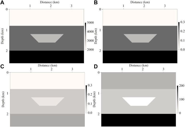
FIGURE 1. The gas block model. (A) Velocity model, (B) $ϵ$ model, (C) $\delta$ model, and (D) Q model.

FIGURE 2

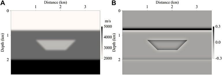
FIGURE 2. Migration and reference reflectivity models of the gas block model. (A) Migration velocity model, and (B) reference reflectivity model.

For the gas block model, we display the RTM images based on different methods in Figure 3, which are isotropic RTM, viscoacoustic RTM, VTI RTM, and viscoacoustic VTI RTM, respectively. In the isotropic RTM image (shown in Figure 3A), it can be seen that due to the absence of anisotropic correction and attenuation compensation, there are imaging noises and structural artifacts, and the diffraction wave cannot converge. The energy of the deep events is weak, and the quality of the image is poor. In the viscoacoustic RTM image (shown in Figure 3B), the energy of the deep layers is effectively restored, and the events are clearer. However, without considering the influence of anisotropy, the diffraction wave cannot be accurately imaged, resulting in certain imaging interference. In the result of the VTI RTM (shown in Figure 3C), the anisotropic migration imaging can effectively suppress the imaging noise and artifacts, and make the diffraction wave accurately homing. However, due to ignoring the absorption attenuation of the medium, the energy of the deep events is weak and the image is not clear enough. In the result of viscoacoustic VTI RTM (shown in Figure 3D), the imaging result can be regarded as an uncompensated VTI RTM image. The diffraction wave in the image converges and the imaging position of the reflection interface is more accurate. The deep energy is not restored, and the energy of the events is weak and not clear. There are low-frequency noise interference and unbalanced energy distribution in the imaging results of all methods.

FIGURE 3

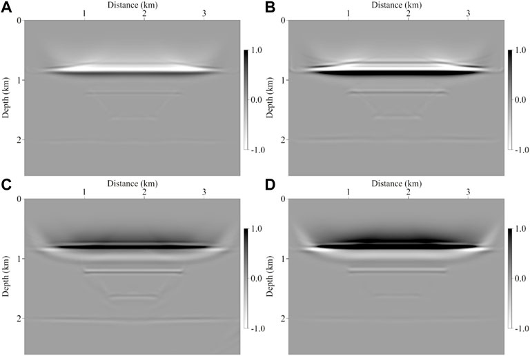
FIGURE 3. RTM images obtained by different methods of the gas block model. (A) Isotropic RTM image, (B) viscoacoustic RTM image, (C) VTI RTM image, and (D) viscoacoustic VTI RTM image. And the color scales of all the images are the same.

Figure 4 shows the LSRTM images based on different methods for the gas block model, which are isotropic LSRTM, viscoacoustic LSRTM, VTI LSRTM, and viscoacoustic VTI LSRTM, respectively. It can be seen that the low-frequency noise and artifacts in the profile are effectively suppressed, the energy distribution is balanced, and the resolution of the image is improved. Compared with the imaging results in Figure 3, it can be found that the viscoacoustic VTI LSRTM approximates the Hessian inverse by iteration, which can effectively compensate for the absorption attenuation. Meanwhile, the resolution and amplitude fidelity of the migration results obtained by the proposed imaging method are higher than those obtained by other methods, which shows that the viscoacoustic VTI LSRTM can accurately image the underground reflection interface, balance the amplitude of the profile, improve the profile resolution and quality.

FIGURE 4

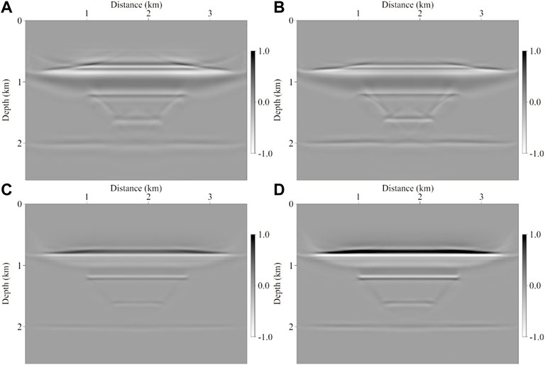
FIGURE 4. LSRTM images obtained by different methods of the gas block model. (A) LSRTM image, (B) viscoacoustic LSRTM image, (C) VTI LSRTM image, and (D) viscoacoustic VTI LSRTM image. And the color scales of all the images are the same.

Figure 5 displays the waveforms extracted from Figure 4 in the same range of x = 1.8 km, z = [1.5, 2.1] km. It can be seen that the VTI-Q-LSRTM can not only compensate for the energy loss, but also correct the phase distortion.

FIGURE 5

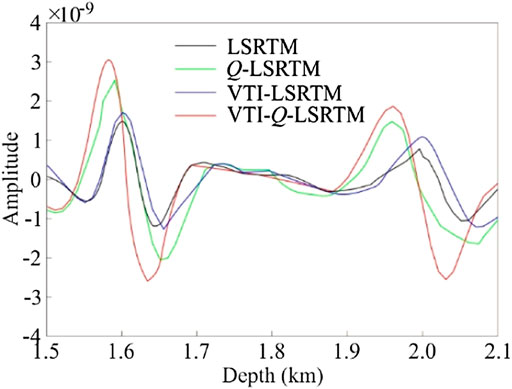
FIGURE 5. Comparison of waveforms extracted from Figure 4, which are in the range of x=1.8 km, z = [1.5, 2.1] km. The curves denote waveforms of LSRTM (black), viscoacoustic LSRTM (green), viscoacoustic VTI LSRTM (blue), and viscoacoustic VTI LSRTM (red), respectively.

Figure 6 displays the normalized convergence curve comparison of the gas block model based on different LSRTM methods. Among them, the black curve is normalized data residuals of the LSRTM, the green curve is normalized data residuals of the viscoacoustic LSRTM, the blue curve is normalized data residuals of the VTI LSRTM, and the red curve is normalized data residuals of the viscoacoustic VTI LSRTM. It can be discovered that the viscoacoustic VTI LSRTM has the fastest convergence speed and the best convergence effect. All these results demonstrate that the viscoacoustic VTI LSRTM proposed in this paper can effectively correct the influence of anelasticity and anisotropy on the migration results, improve the imaging quality, and provide an image with higher resolution, more balanced energy, and fewer artifacts.

FIGURE 6

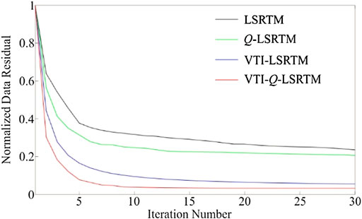
FIGURE 6. Convergence curves of different LSRTM for the gas block model. The curves denote normalized data residuals of LSRTM (black), viscoacoustic LSRTM (green), viscoacoustic VTI LSRTM (blue), and viscoacoustic VTI LSRTM (red), respectively.

Hess model

In this section, the Hess model shown in Figure 7 is employed to verify the effectiveness and applicability of the proposed algorithm in complex models. The model size is 9000 m $\times$ 3750 m, and with a spatial interval of 10 m in both directions. A total of 90 shots are deployed, with the starting point at (0 m, 0 m) and a shot interval of 100 m. Each shot has 451 receivers, with an average distribution on both sides of the source and a channel spacing of 10 m. The length of the seismic record is 4.0 s, and the time sampling interval is 0.5 ms. The zero-phase Ricker wavelet with a dominant frequency of 30 Hz is used as the source function.

FIGURE 7

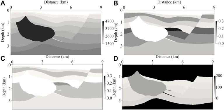
FIGURE 7. The Hess model. (A) Velocity model, (B) $ϵ$ model, (C) $\delta$ model, and (D) Q model.

Figure 8 is the comparison of acoustic and viscoacoustic VTI seismic records of the Hess model. It can be seen that the viscoacoustic VTI seismic record can more accurately reflect the distortion of seismic waveform caused by the anisotropy of the medium, as well as the energy attenuation and phase dispersion caused by the viscosity of the medium. And it indicates that only by thoroughly considering the medium properties can the propagation characteristics of the seismic wave be accurately described, hence providing an accurate data basis for the seismic data imaging processing.

FIGURE 8

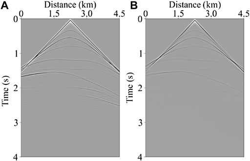
FIGURE 8. The 45th common-shot gather of the Hess model. (A) Acoustic record, and (B) Viscoacoustic VTI record.

Based on the viscoacoustic VTI synthetic data, we perform the migration imaging with four different methods, which are isotropic LSRTM, viscoacoustic LSRTM, VTI LSRTM, and viscoacoustic VTI LSRTM, respectively. Figures 9, 10 show the migration images of the Hess model at the 1st and 30th iterations, respectively. In the RTM image (shown in Figure 9), there are low-frequency noise and artifacts in the shallow layer, the energy of the deep events is weak, and the imaging performance is imperfect. After the LSRTM imaging (shown in Figure 10), the shallow imaging noise and artifacts are suppressed, the overall energy distribution of the profile is more balanced, and the imaging quality is improved significantly. By comparing the LSRTM results with different methods, it can be seen that after anisotropic correction and attenuation compensation, the energy in the middle and deep layers is obviously compensated, and high-quality imaging can be obtained below the attenuation region. The description of the middle-deep structure is clearer and more continuous, the diffraction wave converges, the reflection interfaces can be accurately positioned, and the description of faults and pinch-out structures is more refined. Overall, viscoacoustic VTI LSRTM can effectively improve the resolution and quality of the imaging profile. The advantages of viscoacoustic VTI LSRTM are more detailed in Figure 11 (zoomed views of Figure 9) and Figure 12 (zoomed views of Figure 10).

FIGURE 9

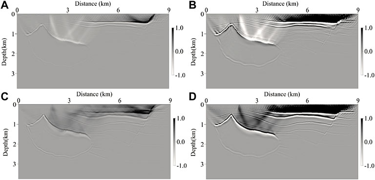
FIGURE 9. RTM images obtained by different methods of the Hess model. (A) Isotropic RTM image, (B) viscoacoustic RTM image, (C) VTI RTM image, and (D) viscoacoustic VTI RTM image. And the color scales of all the images are the same.

FIGURE 10

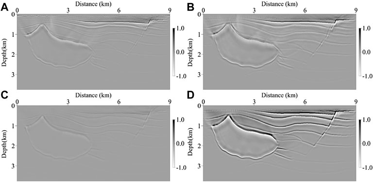
FIGURE 10. LSRTM images obtained by different methods of the Hess model. (A) LSRTM image, (B) viscoacoustic LSRTM image, (C) VTI LSRTM image, and (D) viscoacoustic VTI LSRTM image. And the color scales of all the images are the same.

FIGURE 11

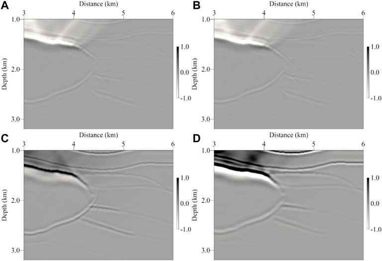
FIGURE 11. Zoomed views of RTM images shown in Figure 9. (A) Isotropic RTM image, (B) viscoacoustic RTM image, (C) VTI RTM image, and (D) viscoacoustic VTI RTM image. And the color scales of all the images are the same.

FIGURE 12

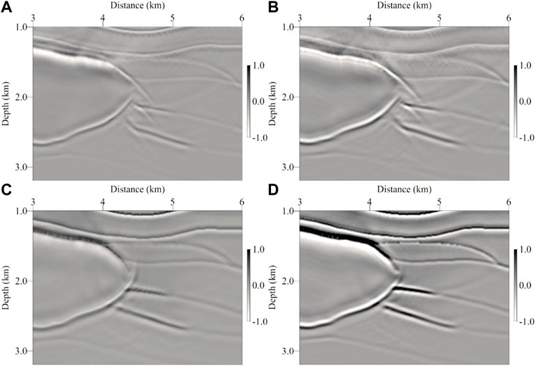
FIGURE 12. Zoomed views of LSRTM images shown in Figure 10. (A) LSRTM image, (B) viscoacoustic LSRTM image, (C) VTI LSRTM image, and (D) viscoacoustic VTI LSRTM image. And the color scales of all the images are the same.

To further reflect the advantages of the LSRTM proposed in this paper, we compare the wavenumber spectrum (shown in Figure 13) of the imaging results. The first row is the wavenumber spectrum of the RTM images (from Figure 9), and the second row is the wavenumber spectrum of the LSRTM images (from Figure 10). Compared with the wavenumber spectrum of the same row, it can be found that the wavenumber spectrum of anisotropic and attenuation compensation imaging contains more abundant wavenumber components, and the high-wavenumber components in the imaging profile are widened. By comparing the wavenumber spectra of the same column, it can be found that compared with the RTM results, the wavenumber components contained in the LSRTM results are more comprehensive, and the low-wavenumber components are supplemented, which indicates that the resolution and quality of the viscoacoustic VTI LSRTM image after multiple iterations are improved.

FIGURE 13

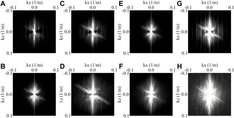
FIGURE 13. Wavenumber spectrum comparison of images shown in Figures 8, 9 for the Hess model. (A) RTM, (B) LSRTM, (C) viscoacoustic RTM, (D) viscoacoustic LSRTM, (E) VTI RTM, (F) VTI LSRTM, (G) viscoacoustic VTI RTM, and (H) viscoacoustic VTI LSRTM. And the color scales of all the images are the same.

Figure 14 displays the comparison of the 45th Born modeling common-shot gather calculated by the RTM (shown in the first row) of the Hess model and the LSRTM (shown in the second row). Among them, from left to right are the Born modeling records calculated by the isotropic, viscoacoustic, VTI, and viscoacoustic VTI wave equation, respectively. Compared with the Born modeling records under different iterations (shown in the same column), it can be seen that the Born modeling records obtained by LSRTM contain more reflection events, the waveform information is richer, the reflectivity profile is corrected, and the Born modeling records are gradually consistent with the real records. By comparing the Born modeling records of the same row, it can be found that the events energy of the Born modeling record obtained by viscoacoustic VTI imaging is restored, the wavefield contains more anisotropic information, and the events are richer and clearer.

FIGURE 14

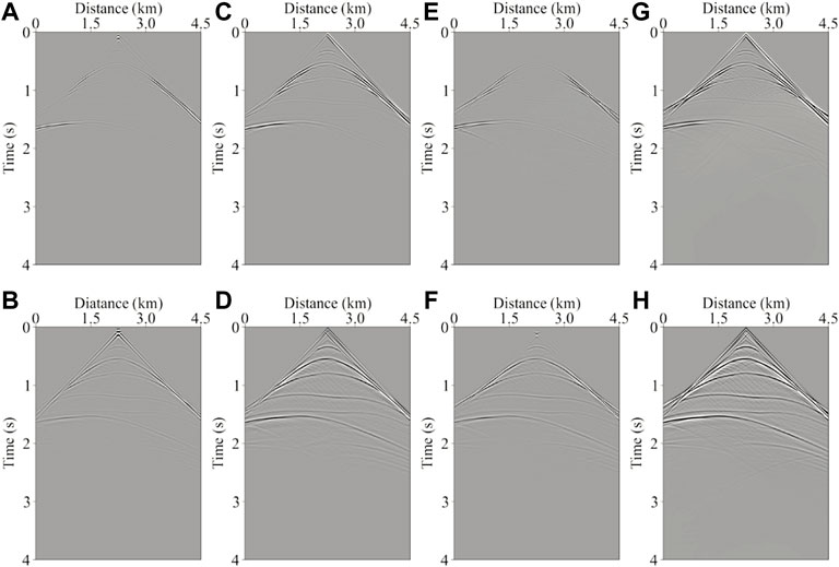
FIGURE 14. The 45th Born modeling common-shot gather of the Hess model. (A) RTM, (B) LSRTM, (C) viscoacoustic RTM, (D) viscoacoustic LSRTM, (E) VTI RTM, (F) VTI LSRTM, (G) viscoacoustic VTI RTM, and (H) viscoacoustic VTI LSRTM. And the color scales of all the images are the same.

Figure 15 displays the convergence curves of the LSRTM for the Hess model under different imaging methods. Among them, the black, green, blue, and red curves represent the convergence curves of the isotropic, viscoacoustic, VTI, and viscoacoustic VTI LSRTM, respectively. From the comparison of different curves, it can be found that in the previous iterations, the objective function of the four migration methods decline rapidly, among which the decline rate of isotropic LSRTM is the slowest, and the decline rate of viscoacoustic VTI LSRTM is the fastest. After more iterations, the decline rate of the objective function gradually becomes slower, and the imaging method without attenuation compensation gradually stabilizes to about 0.3, while the imaging method with attenuation compensation decreases to less than 0.2. The convergence rate of viscoacoustic VTI LSRTM is the fastest, and its relative error converges to the minimum, indicating that the consistency between the imaging profile and the reference reflectivity profile is the highest, and the imaging quality is the best.

FIGURE 15

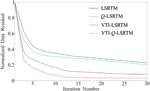
FIGURE 15. Convergence curves of different LSRTM for Hess model. The curves denote normalized data residuals of LSRTM (black), viscoacoustic LSRTM (green), viscoacoustic VTI LSRTM (blue), and viscoacoustic VTI LSRTM (red), respectively.

Field data test

To further verify the practicability of the viscoacoustic VTI LSRTM method in the field data, this section is based on the field data collected in Bohai Bay. Figure 16 shows the field data migration parameters, where the model size is 15 km $\times$ 5 km. The migration velocity field and anisotropic parameters of the data are obtained by the multi-parameter tomography modeling method. The quality factor Q is calculated by the empirical equation $Q=3.516v^{2.2}$ from the velocity field, and the minimum value is 20, indicating that there is a strong attenuation medium in the working zone. A total of 399 shots of data are collected, with a total of 1300 channels per shot. The time interval of each channel is 2 ms, the total length of recording is 4.0 s, the interval between channels is 12.5 m, and the interval between shots is 37 m. The right excitation method is adopted. In the wavefield propagation of viscoacoustic VTI LSRTM, the number of horizontal and vertical grid points is 1801 $\times$ 1001, the spatial interval is 12.5 m in horizontal and 5.0 m in vertical, the time interval is 1.0 ms, and the dominant frequency is 20 Hz Rick wavelet is used as the source function.

FIGURE 16

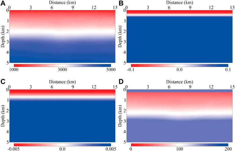
FIGURE 16. Migration models of the field data. (A) Velocity model, (B) $ϵ$ model, (C) $\delta$ model, and (D) Q model.

We display the migration results of the field data in Figure 17, where Figure 17A displays the viscoacoustic VTI RTM and Figure 17B displays the viscoacoustic VTI LSRTM, respectively. Compared with the migration results, it can be discovered that the low-frequency noise in the shallow layer and the structural illusion in the profile are well suppressed in the viscoacoustic VTI LSRTM image. The fault structure is more detailed, the imaging is more clear and accurate, the breakpoints are clearly depicted, and the continuity of the section is enhanced. The imaging quality of the thin layers in the shallow region is improved, and the resolution of the events is enhanced. The energy in the middle and deep layers is well recovered after compensation, the events are more continuous and clearer, and its structural form is well characterized. Therefore, viscoacoustic VTI LSRTM proposed can improve formation imaging quality.

FIGURE 17

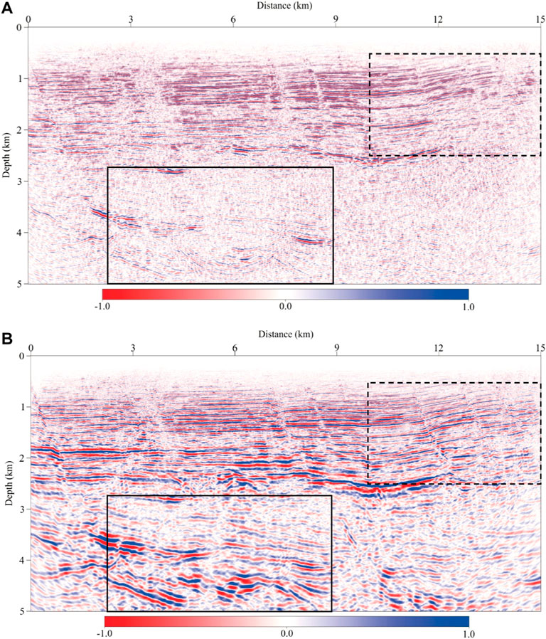
FIGURE 17. Migration images of field data. (A) Viscoacoustic VTI RTM, and (B) viscoacoustic VTI LSRTM. And the color scales of all the images are the same.

Figure 18 shows the zoomed views for the black dashed box area in Figure 17. The area is located in the shallow and middle layers of the field data, and there are rich fault structures. It can be seen that the region can be imaged through RTM, but the energy of the events in the profile is weak, and the overall amplitude is not balanced. In the fault region, the imaging of some faults is not clear and accurate, the continuity of the section is not strong, and the breakpoint is not clear. In the LSRTM image, the energy of the events is restored and enhanced, the energy distribution of the profile is more balanced, and the resolution is improved. In the fault region, the imaging of the faults is clearer and more accurate, the continuity of the section is enhanced, the characterization of the breakpoint is clearer, and the overall imaging quality is improved.

FIGURE 18

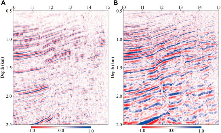
FIGURE 18. Zoomed views of dashed box in Figure 17. (A) Viscoacoustic VTI RTM, and (B) viscoacoustic VTI LSRTM. And the color scales of all the images are the same.

Figure 19 shows the zoomed views for the black solid box area in Figure 17. The region in the box is in a deep position of the field data, and it is difficult to obtain ideal imaging results in conventional processing methods. In the results of RTM, the events of the region are obviously disordered, the energy is weak, and there are serious artifacts. After several iterations of viscoacoustic VTI LSRTM, anisotropy and attenuation are corrected at the same time, the deep energy is compensated and restored, the diffraction wave is better convergent and homing, the artifacts are suppressed, the energy of the events is better focused, and the imaging is more continuous and clear. The imaging resolution and quality of the profile are improved.

FIGURE 19

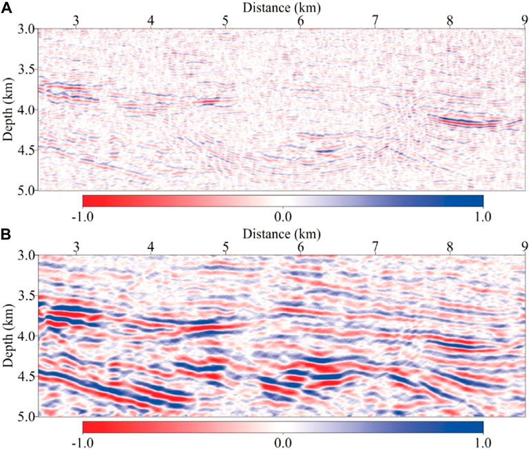
FIGURE 19. Zoomed views of solid box in Figure 17. (A) Viscoacoustic VTI RTM, and (B) viscoacoustic VTI LSRTM. And the color scales of all the images are the same.

To fully reflect the advantages of viscoacoustic VTI LSRTM imaging, we display the wavenumber spectrum of the whole migration images in Figure 20, where Figures 20A,B are the wavenumber spectrum of the VTI LSRTM result and viscoacoustic VTI LSRTM result, respectively. From the comparison of the two images, it can be seen that after iterations, the low wavenumber and high wavenumber components in the imaging results have been supplemented, the wavenumber range has been widened to a certain extent, and the wavenumber components in the profile are more comprehensive and richer, which shows that the resolution of the viscoacoustic VTI LSRTM image is improved.

FIGURE 20

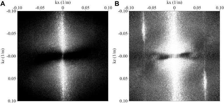
FIGURE 20. Comparison of wavenumber spectra of field data imaging results. (A) Viscoacoustic VTI RTM, and (B) viscoacoustic VTI LSRTM. And the color scales of all the images are the same.

Figure 21 is the comparison between field data and the 316th Born modeling common-shot gather after multiple iterations, where Figure 21A is the field data, Figure 21B is the Born modeling common-shot gather of VTI RTM, and Figure 21C is the Born modeling common-shot gather of viscoacoustic VTI LSRTM. Compared to the field data, the common-shot gather calculated by VTI RTM contains fewer reflection wave events, whose waveform is similar to the field data. However, the energy of these events is weaker while the resolution is lower, which is not matched well with the field data. In the contrast, there are significant improvements in the events in the viscoacoustic VTI LSRTM Born modeling common-shot gather. The record contains more abundant waveform information and the energy of the events is compensated and restored, whose resolution is somewhat enhanced. And the wavefield is matched well with the field data, which demonstrates the correctness and effectiveness of the proposed imaging method.

FIGURE 21

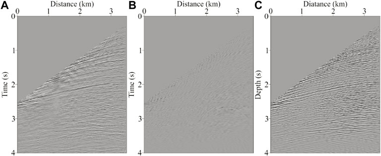
FIGURE 21. Comparison between field data and Born modeling wavefield. (A) Field data, (B) the 316th Born modeling common-shot gather of viscoacoustic VTI RTM, and (C) the 316th Born modeling common-shot gather of viscoacoustic VTI LSRTM.

Figure 22 shows the objective function convergence curve of viscoacoustic VTI LSRTM for the field data. It can be seen that in the previous iterations, the relative error of the objective function rapidly decreased to around 0.3. With the increase of iterations, the decline rate of the relative error gradually slowed down, and finally stabilized below 0.2. This shows that the LSRTM with anisotropy and attenuation compensation can continuously optimize the objective function by iteration, provide a more consistent reflectivity profile with the actual, and can achieve better imaging results in practical data applications.

FIGURE 22

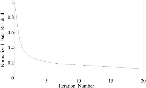
FIGURE 22. Convergence curve of the field data.

Discussion

The dependence analysis of least-squares reverse time migration on migration parameters

In the process of LSRTM, the selection of imaging parameters, imaging conditions, and seismic wavelets will have different degrees of influence on imaging accuracy. In this section, the effects of the migration velocity field, anisotropic parameters, quality factor Q, and wavelet selection on imaging accuracy are compared, and other factors are the same.

Figure 23 shows the imaging results of the Hess model under different migration parameters. By comparing Figures 23A,B, it can be seen that when the migration velocity is 10% lower than the real velocity, the depth value of each interface becomes smaller, and the deep imaging is seriously distorted, which cannot accurately reflect the form of underground structure. When the migration velocity is 10% higher than the real velocity, the depth of each interface becomes larger, and the general structural shape changes little. The depth change after the migration velocity increases is larger than that after the migration velocity decreases, but the structural shape changes little. Compared with the case of small velocity, the change in the general structure of the imaging results is smaller and the change in the depth position is more obvious when the migration velocity is larger.

FIGURE 23

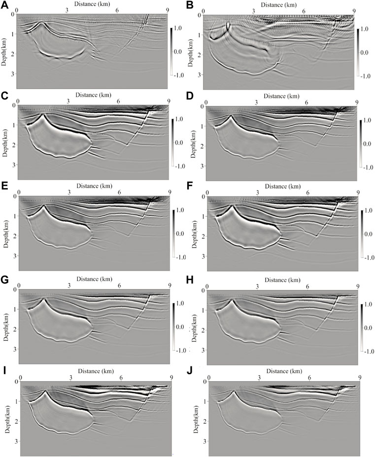
FIGURE 23. Error analysis of the LSRTM parameters for the Hess model. (A) 10% decrease in velocity, (B) 10% increase in velocity, (C) 10% decrease in $ϵ$, (D) 10% increase in $ϵ$, (E) 10% decrease in $\delta$, (F) 10% increase in$\delta$, (G) 10% decrease in Q, and (H) 10% increase in Q, (I) 30° phase rotation of wavelet, (J) 90° phase rotation of wavelet. And the color scales of all the images are the same.

In the error comparison of anisotropic parameters (shown in Figures 23C–F), it can be seen that the change of anisotropic parameters has a certain influence on the migration results. When the anisotropic parameters are inaccurate, imaging noise interference and imaging position error will occur in the imaging profile. In theory, the anisotropic parameter $\mathrm{\epsilon }$ is related to the transverse propagation velocity of the seismic wave, and the parameter $\delta$ determines the correction velocity of the P-wave relative to the symmetric axis. In the case of ignoring the perturbation of anisotropic parameters, the influence on the imaging profile is not obvious compared with the influence of velocity error.

In the parameter error comparison of the quality factor (shown in Figures 23G,H), it can be seen that the change in the quality factor has a certain influence on the migration results. When the perturbation of the quality factor is ignored, the influence of the quality factor error within a certain range on the imaging profile is weaker than that of the velocity error. When the quality factor error exceeds a certain range, it will cause insufficient energy compensation and incomplete phase distortion correction in the profile. Therefore, it is necessary to make a relatively accurate estimation of the quality factor model to show that the attenuation compensation can significantly improve the quality of imaging results.

According to Zhang et al. (2016), the source-independent LSRTM is insensitive to the source wavelet and can still produce an amplitude-preserving image even using an incorrect wavelet without the source estimation. Due to the wavelet after 30° phase rotation, the wavelet with a little time shift and amplitude errors is similar to the original true wavelet, the LSRTM can obtain a satisfactory image (Figure 23I). When the wavelet after 90° phase rotation is used, the LSRTM image becomes blurring (Figure 23J), but still is an amplitude-preserving image. Compared to the velocity error, it can be seen that the proposed LSRTM algorithm is insensitive to the phase of the source wavelet.

Overall, the imaging profile is most sensitive to the accuracy of the migration velocity field, and the sensitivity to anisotropic parameters, quality factor, and the phase of the source wavelet are relatively low. Therefore, the imaging quality of LSRTM is affected by migration velocity, medium anisotropy, and quality factor. Accurate migration parameters and the development of attenuation anisotropy RTM imaging methods can achieve high-quality imaging results.

Conclusion

Based on the viscoacoustic VTI pure qP-wave equation, we deduce the demigration operator, adjoint operator, and gradient sensitivity-kernel, and construct the LSRTM algorithm in the viscoacoustic VTI medium. In the implementation process of this algorithm, the adjoint wavefield keeps attenuation which can avoid the instability caused by the exponential growth of high-frequency components energy. Numerical examples of synthetic and field data demonstrate that the proposed method can perform high-quality imaging in the attenuation region, enrich the wavenumber components, broaden the bandwidth in the imaging profile, and improve the imaging resolution and accuracy of the underground medium. Through the analysis and comparison of parameter errors, it can be seen that compared with the anisotropic parameters and quality factor Q, the LSRTM method is most sensitive to the migration velocity. Therefore, improving the accuracy of migration parameters can effectively improve the quality of the imaging profile.

Data availability statement

The original contributions presented in the study are included in the article/Supplementary Material, further inquiries can be directed to the corresponding author.

Author contributions

SZ and BG contributed to the conception and design of the study. SZ organized the database and performed the statistical analysis. ZL modified the manuscript. All authors have read the manuscript and agreed to publish it.

Funding

This research is supported by the National Natural Science Foundation of China (grant nos. 42004093, 42074133), the Major Scientific and Technological Projects of CNPC (no. ZD 2019-183-003), and the Shandong Province Natural Science Foundation, China (grant no. ZR2020QD050).

Acknowledgments

The authors are grateful to the editors and reviewers for their review of this manuscript. Meanwhile, the authors would like to thank the SWPI group for providing excellent support for this reaearch.

Conflict of interest

The authors declare that the research was conducted in the absence of any commercial or financial relationships that could be construed as a potential conflict of interest.

Publisher’s note

All claims expressed in this article are solely those of the authors and do not necessarily represent those of their affiliated organizations, or those of the publisher, the editors and the reviewers. Any product that may be evaluated in this article, or claim that may be made by its manufacturer, is not guaranteed or endorsed by the publisher.

References

Alkhalifah, T. (1998). Acoustic approximations for processing in transversely isotropic media. Geophysics 63 (2), 623–631. doi:10.1190/1.1444361

CrossRef Full Text | Google Scholar

Bai, J. Y., Chen, G. Q., and Yingst, D. (2013). “Attenuation compensation in viscoacoustic reverse time migration,” in Proceeding of the 83rd Annual International Meeting, Texas United States, 19 Aug 2013 (Houston, TX: SEG), 3825–3830. doi:10.1190/segam2013-1252.1

CrossRef Full Text | Google Scholar

Baysal, E., Kosloff, D. D., and Sherwood, J. W. (1983). Reverse time migration. Geophysics 48 (11), 1514–1524. doi:10.1190/1.1441434

CrossRef Full Text | Google Scholar

Bickel, S. H., and Natarajan, R. R. (1985). Plane wave Q deconvolution. Geophysics 50 (9), 1426–1439. doi:10.1190/1.1442011

CrossRef Full Text | Google Scholar

Chai, X. T., Wang, S. X., Tang, G. Y., and Meng, X. (2017). Stable and efficient Q-compensated least-squares migration with compressive sensing, sparsity-promoting, and preconditioning. J. Appl. Geophys. 145, 84–99. doi:10.1016/j.jappgeo.2017.07.015

CrossRef Full Text | Google Scholar

Chen, H. M., Zhou, H., and Tian, Y. K. (2020). Least-squares reverse-time migration based on a fractional Laplacian viscoacoustic wave equation. Oil Geophys. Prospect. (in Chin. 55 (3), 616–626.

Google Scholar

Chen, Y. Q., Dutta, G., Dai, W., and Schuster, G. T. (2017). Q-least-squares reverse time migration with viscoacoustic deblurring filters. Geophysics 82 (6), S425–S438. doi:10.1190/geo2016-0585.1

CrossRef Full Text | Google Scholar

Cheng, J. B., and Kang, W. (2016). Simulating propagation of separated wave modes in general anisotropic media, Part II: qS-wave propagators. Geophysics 81 (2), C39–C52. doi:10.1190/geo2015-0253.1

CrossRef Full Text | Google Scholar

Cheng, J. B., Kang, W., and Wang, T. F. (2013). Description of qP-wave propagation in anisotropic media. Part Ⅰ: Pseudo-pure-mode wave equations. Chin. J. Geophys. (in Chinese) 56 (10), 3474–3486. doi:10.6038/cjg20131022

CrossRef Full Text | Google Scholar

Chu, C. L., Macy, B. K., and Anno, P. D. (2011). Approximation of pure acoustic seismic wave propagation in TTI media. Geophysics 76 (5), WB97–WB107. doi:10.1190/geo2011-0092.1

CrossRef Full Text | Google Scholar

Du, X., Bancroft, J. C., and Lines, L. R. (2007). Anisotropic reversetime migration for tilted TI media. Geophys. Prospect. 55 (6), 853–869. doi:10.1111/j.1365-2478.2007.00652.x

CrossRef Full Text | Google Scholar

Dutta, G., and Schuster, G. T. (2014). Attenuation compensation for least-squares reverse time migration using the viscoacoustic-wave equation. Geophysics 79 (6), S251–S262. doi:10.1190/geo2013-0414.1

CrossRef Full Text | Google Scholar

Dvorkin, J. P., and Mavko, G. (2006). Modeling attenuation in reservoir and nonreservoir rock. The Leading Edge 25 (2), 194–197. doi:10.1190/1.2172312

CrossRef Full Text | Google Scholar

Fathalian, A., Trad, D. O., and Innanen, K. A. (2021). Q-compensated reverse time migration in tilted transversely isotropic media. Geophysics 86 (1), S73–S89. doi:10.1190/geo2019-0466.1

CrossRef Full Text | Google Scholar

Fomel, S. (1996). Least-square inversion with inexact adjointsMethod of conjugate direction: A tutorial. Stanf Explor Proj 92, 253–265.

Google Scholar

Gu, B. L., Li, Z. C., and Han, J. G. (2018). A wavefield-separation-based elastic least-squares reverse time migration. Geophysics 83 (3), S279–S297. doi:10.1190/geo2017-0131.1

CrossRef Full Text | Google Scholar

Guo, P., Guan, H. M., Nammour, R., and Duquet, B. (2017). “A stable Q compensation approach for adjoint seismic imaging by pseudodifferential scaling,” in Proceeding of the 87th Annual International Meeting, Texas United States, 17 Aug 2017 (SEG), 4566–4571. doi:10.1190/segam2017-17747338.1

CrossRef Full Text | Google Scholar

Guo, P., McMechan, G. A., and Guan, H. (2016). Comparison of two viscoacoustic propagators for Qcompensated reverse time migration. Geophysics 81 (5), S281–S297. doi:10.1190/geo2015-0557.1

CrossRef Full Text | Google Scholar

Hargreaves, N. D., and Calvert, A. J. (1991). Inverse Q filtering by Fourier transform. Geophysics 56 (4), 519–527. doi:10.1190/1.1443067

CrossRef Full Text | Google Scholar

He, B. S., Gao, K. P., and Xu, G. H. (2021). Elastic wave reverse time migration in anisotropic media: State of the art and perspectives. Geophysical Prospecting for Petroleum 61 (2), 210–223.

Google Scholar

Li, X. Y., and Zhu, H. J. (2018). A finite-difference approach for solving pure quasi-P wave equations in transversely isotropic and orthorhombic media. Geophysics 83 (4), C161–C172. doi:10.1190/geo2017-0405.1

CrossRef Full Text | Google Scholar

Li, Z. C., and Wang, Q. Z. (2007). A review of research on mechanism of seismic attenuation and energy compensation. Progress in Geophys 22 (4), 1147–1152.

Google Scholar

Liu, F. Q., Morton, S. A., Jiang, S. S., Ni, L., and Leveille, J. P. (2009). “Decoupled wave equations for P and SV waves in an acoustic VTI media,” in Proceeding of the 79th Annual International Meeting, Texas United States, 14 Oct 2009 (SEG), 2844–2848. doi:10.1190/1.3255440

CrossRef Full Text | Google Scholar

McMechan, G. A. (1983). Migration by extrapolation of time-dependent boundary values. Geophys. Prospect. 31 (3), 413–420. doi:10.1111/j.1365-2478.1983.tb01060.x

CrossRef Full Text | Google Scholar

Mittet, R., Sollie, R., and Hokstad, K. (1995). Prestack depth migration with compensation for absorption and dispersion. Geophysics 60 (5), 1485–1494. doi:10.1190/1.1443882

CrossRef Full Text | Google Scholar

Nemeth, T., Wu, C. J., and Schuster, G. T. (1999). Least-squares migration of incomplete reflection data. Geophysics 64 (1), 208–221. doi:10.1190/1.1444517

CrossRef Full Text | Google Scholar

Qu, Y. M., Wang, Y. X., Li, Z. C., and Liu, C. (2021). Q least-squares reverse time migration based on the first-order viscoacoustic quasidifferential equations. Geophysics 86 (4), S283–S298. doi:10.1190/geo2020-0712.1

CrossRef Full Text | Google Scholar

Robertsson, J. O., Blanch, J. O., and Symes, W. W. (1994). Viscoelastic finite-difference modeling. Geophysics 59 (9), 1444–1456. doi:10.1190/1.1443701

CrossRef Full Text | Google Scholar

Sun, J. Z., Fomel, S., Zhu, T. Y., and Hu, J. (2016). Q-compensated least-squares reverse time migration using low-rank one-step wave extrapolation. Geophysics 81 (4), S271–S279. doi:10.1190/geo2015-0520.1

CrossRef Full Text | Google Scholar

Sun, J. Z., and Zhu, T. Y. (2018). Strategies for stable attenuation compensation in reverse time migration. Geophysical Prospecting 66 (3), 498–511. doi:10.1111/1365-2478.12579

CrossRef Full Text | Google Scholar

Thomsen, L. (1986). Weak elastic anisotropy. Geophysics 51 (10), 1954–1966. doi:10.1190/1.1442051

CrossRef Full Text | Google Scholar

Tian, K., Huang, J. P., Bu, C., Guolei, L., Xinhua, Y., Jinfeng, L., et al. (2015). “Viscoacoustic reverse time migration by adding a regularization term,” in Proceeding of the 85th Annual International Meeting, Texas United States, 19 Aug 2015 (SEG), 4127–4131. doi:10.1190/segam2015-5932246.1

CrossRef Full Text | Google Scholar

Valenciano, A., Chemingui, N., Whitmore, D., and Brandsberg-Dahl, S. (2011). “Wave equation migration with attenuation and anisotropy compensation,” in Proceeding of the 81st Annual International Meeting, Texas United States, 08 Aug 2011 (SEG), 232–237. doi:10.1190/1.3627674

CrossRef Full Text | Google Scholar

Wang, E. J., and Ba, J. (2018). “Q-compensated reverse time migration and least square reverse time migration methods,” in Proceeding of the 88th Annual International Meeting, Texas United States, 27 Aug 2018 (SEG), 4503–4507. doi:10.1190/segam2018-2996850.1

CrossRef Full Text | Google Scholar

Wang, Y. H. (2008). Inverse-Q filtered migration. Geophysics 73 (1), S1–S6. doi:10.1190/1.2806924

CrossRef Full Text | Google Scholar

White, J. E. (1975). Computed seismic speeds and attenuation in rocks with partial gas saturation. Geophysics 40 (2), 224–232. doi:10.1190/1.1440520

CrossRef Full Text | Google Scholar

Wu, G. C. (2006). Seismic wave propagation and imaging in anisotropic media in Chinese. Dongying: China University of Petroleum Press.

Google Scholar

Xie, Y., Xin, K., Sun, J. Z., Notfors, Y., Biswal, A., and Balasubramaniam, M. (2009). “3D prestack depth migration with compensation for frequency dependent absorption and dispersion,” in Proceeding of the 79th Annual International Meeting, Texas United States, 14 Oct 2009 (SEG), 2919–2923. doi:10.1190/1.3255457

CrossRef Full Text | Google Scholar

Xu, S. B., Stovas, A., Alkhalifah, T., and Mikada, H. (2020). New acoustic approximation for transversely isotropic media with a vertical symmetry axis. Geophysics 85 (1), C1–C12. doi:10.1190/geo2019-0100.1

CrossRef Full Text | Google Scholar

Xu, S., and Zhou, H. B. (2014). Accurate simulations of pure quasi-P-waves in complex anisotropic media. Geophysics 79 (6), T341–T348. doi:10.1190/geo2014-0242.1

CrossRef Full Text | Google Scholar

Zhang, Q. C., Zhou, H., Chen, H. M., and Wang, J. (2016). Least-squares reverse time migration with and without source wavelet estimation. Journal of Applied Geophysics 134, 1–10. doi:10.1016/j.jappgeo.2016.08.003

CrossRef Full Text | Google Scholar

Zhang, S. S., Gu, B. L., Ding, Y., Wang, J., and Li, Z. (2022). Reverse time migration of viscoacoustic anisotropic pure qP-wave based on nearly constant Q model. Chinese J. Geophysics. doi:10.6038/cjg2022P0570

CrossRef Full Text | Google Scholar

Zhang, Y., Zhang, H. Z., and Zhang, G. Q. (2011). A stable TTI reverse time migration and its implementation. Geophysics 76 (3), WA3–WA11. doi:10.1190/1.3554411

CrossRef Full Text | Google Scholar

Zhang, Y., Zhang, P., and Zhang, H. Z. (2010). “Compensating for visco-acoustic effects with reverse time migration,” in Proceeding of the 80ed Annual International Meeting, Texas United States, 21 Oct 2010 (SEG), 3160–3164. doi:10.1190/1.3513503

CrossRef Full Text | Google Scholar

Zhao, X. B., Zhou, H., Wang, Y. F., Chen, H., Zhou, Z., Sun, P., et al. (2018). A stable approach for Q-compensated viscoelastic reverse time migration using excitation amplitude imaging condition. Geophysics 83 (5), S459–S476. doi:10.1190/geo2018-0222.1

CrossRef Full Text | Google Scholar

Zhu, T. Y., Harris, J. M., and Biondi, B. (2014). Q-compensated reverse-time migration. Geophysics 79 (3), S77–S87. doi:10.1190/geo2013-0344.1

CrossRef Full Text | Google Scholar