A numerical study of 3D topographic site effects considering wavefield incident direction and geomorphometric parameters

The topographic site effect plays a vital role in controlling the characteristics of earthquake ground motions. Due to its complexity, the factors affecting topographic amplification have not been fully identified. In this study, 100 ground motion simulations generated by double-couple point sources in the homogeneous linear elastic half-space are performed based on the 3D (three-dimensional) Spectral Element Method, taking the Menyuan area of Qinghai Province, China as a local testbed site. A relationship between incident direction and the strength of topographic amplification has been observed. The horizontal ground motion is affected by the back-azimuth, which is typically chosen to be the direction from seismic station to seismic source measured clockwise from north. Specifically, the east-west PGA (Peak Ground-motion Acceleration) is significantly amplified when back-azimuth is about $90°$ or $270°$, and the north-south PGA is significantly amplified when back-azimuth is around $0°$ or $180°$. The vertical ground motion is affected by the dipping angle, which is the angle from vertical at which an incoming seismic wave arrives. The vertical PGA is strongly amplified when the seismic wave is almost horizontally incident (e.g., dipping angle = $78°$). A correlation study between geomorphometric parameters and frequency-dependent topographic amplification indicates that relative elevation and smoothed curvature contain similar information, both of which are closely related to the topographic amplification of horizontal components, but not the vertical component. Our study reveals the influence of source and propagation path on topographic amplification and provides a reference for considering the topographic site effect in real engineering sites.

Introduction

The topographic site effect refers to the scattering of seismic waves by topographic irregularities, which generally manifests as the ground motion amplified at the convex features such as hilltops and deamplified at the concave features such as valleys. The interaction between seismic waves and irregular topographic features can be dramatic: a high peak ground acceleration (PGA) of 1.78 g was recorded at the Tarzana hilltop stations during the 1994 Northridge earthquake (Bouchon and Barker, 1996; Ashford and Sitar, 1997); A PGA of 1.25 g recorded by the Pacoima Dam site during the 1971 San Fernando earthquake (Trifunac and Hudson, 1971); For moderate earthquakes, severe damage can also be partially attributed to the scattering effect of topography (e.g., Kang et al. 2019).

Although empirical evidence pointing out the contributions of topography do exist in various seismic scenarios (Hartzell et al., 1994; Harris, 1998; Buech et al., 2010; Hough et al., 2010; Pischiutta et al., 2010; Luo et al., 2014), topographic site effects have received less attention compared with stratigraphic site effects. Topographic site effects are often invoked to explain abnormal ground motion amplitudes in local areas, and its complexity makes the relevant research encounter challenges in reproducing the amplification value accurately. More specifically, the relevant information of the source, propagation path, and engineering site are all covered in the ground motion records. Among these, the site condition includes stratified soil, topography, sedimentary basin structure, etc. To perform quantitative analysis, the contribution of the topography itself needs to be extracted separately from the ground motion records, and the influence of source, stratified soil, and other factors on the topographic amplification value cannot be ignored. Asimaki and Mohammadi (2018) emphasized a non-linear coupling between the amplification effects from surface topography and subsurface stratified soil. The thickness, shear wave velocity, damping ratio, and lateral heterogeneity of the underlying geologic materials all affect the topographic amplification (Assimaki and Gazetas, 2004; Assimaki et al., 2005a; Assimaki et al., 2005b; Bouckovalas and Papadimitriou, 2005; Wang et al., 2019; Luo et al., 2020; Song et al., 2020). The source and propagation path indirectly affect the topographic site effect by determining the azimuth and frequency content of the incoming wavefield, and there are few related studies. Using three-dimensional finite difference methods, Mayoral et al. (2019) indicates that for hill slopes, subduction earthquakes led to deep failure surfaces, whereas normal events to shallow failure surfaces.

At present, there are three kinds of methods to study the topographic site effects: experimental method (e.g., Tucker et al., 1984; Wood and Cox, 2016; Stolte et al., 2017), analytical and semi-analytical method (e.g., Yuan and Liao, 1996; Paolucci, 2002) and numerical simulation methods (e.g., Boore, 1972; Geli et al., 1988; Hartzell et al., 2017). The standard spectral ratio (SSR) method (Borcherdt, 1970) is the spectral ratio of ground motions between the target station and the adjacent reference station. It is widely used in the study of topographic site effects due to its ease of operation and clear physical context, but the reference station needs to be located on the bedrock site and cannot be affected by the adjacent topographic features, which limits the amount of available ground motion data. The Nakamura (HVSR, horizontal-to-vertical spectral ratio) method, which avoids the selection of the reference station by using the horizontal to the vertical spectral ratio of the same station to characterize site effects (Nakamura, 1989). However, the topographic amplification of vertical ground motion reduces the accuracy of the estimation of amplification. Some scholars used microtremors to make up for the lack of ground motion records (e.g., Stolte et al., 2017; La Rocca et al., 2020). Numerical simulations also have helped augment the observational record, but the numerical results are usually smaller than those of experiments (Geli et al., 1988; Lovati et al., 2011). The reason is that the underground shear wave velocity structure and soil layer information are usually unclear, and the accuracy of the elevation data used in the numerical simulation is also limited, which greatly affects the accuracy of the numerical modeling (Moore et al., 2011; Burjánek et al., 2012; Burjánek et al., 2014). However, with the growth in computational capabilities, the development of codes capable of handling complex topographies, and more high-quality near-surface geologic data available, it is becoming easier to directly model ground-motion amplification due to topography. Some studies that consider surface topography has obtained simulation results that are in good agreement with observed ground motions (Magnoni et al., 2013; Galvez et al., 2021; Wang et al., 2021).

In this paper, we first adopt the spectral element method to establish a ground motion synthetic database, and then explore the influence of the incident direction of the incoming seismic wavefield on the topographic amplification; in addition, the correlation between geomorphometric parameters, which commonly used to build the ground-motion models (GMMs), and topographic amplification values have also been analyzed. Finally, we discuss the physical mechanism behind the source-site interaction and make recommendations for considering the topographical site effect in real engineering sites.

Ground-motion synthetic database

A powerful and freely available spectral element software, called SPECFEM3D, is adopted to generate the synthetic ground motion data. The Spectral Element Method (SEM) enjoys the geometrical flexibility of the Finite Element Method and the accuracy of the Pseudo-Spectral Method. High-degree Lagrange interpolants are used to express functions in SEM. Therefore, the accuracy of the simulation can be ensured by adjusting the polynomial degree and the representative element size. The polynomial degree is set to 4 in our study [following Komatitsch et al., 2005; Igel, 2017; Yuan et al., 2021], which means one SEM element per wavelength has been found to be accurate. As a comparison, the spatial element size in some finite difference methods must be smaller than approximately one-tenth to one-eighth of the wavelength, which leads to a great number of elements (e.g., Ma et al., 2021). The SEM allows for systematic diagonalization of the mass matrix, which then allows for easy parallelization.

Menyuan area, Qinghai Province, China is located northeast of the Qinghai Tibet Plateau, with a great difference in elevation and the average elevation is 2,866 m. The overall terrain is high in the northwest, low in the southeast, high in the north and south, and low in the middle. The north is adjacent to the Qilian Mountains, and the Datong River Valley in the middle is relatively flat. As shown in Figure 1A, the topography is complex, including ridges, isolated hills, valleys, canyons, and flat surfaces, which cover a large variety of topographic features often present in real cases in which 3D site effects may occur. Therefore, A 3D model with dimensions of $41\times 44\times 15$ km³ surrounding the Menyuan area is established to understand the mechanism of topographic site effect. The digital elevation data comes from the ASTER Global Digital Elevation Model (GDEM) Version 3, with a spatial resolution of 1 arc-s (approximately 30-m horizontal posting at the equator). 3,721 virtual receivers (black dots in Figure 1B) are regularly distributed in a $30\times 30$ km² area that covers the main topographic features of the computational domain. The ground motion of three components [corresponding to east-west (X), north-south (Y), and vertical (Z)] can be recorded by each receiver.

FIGURE 1

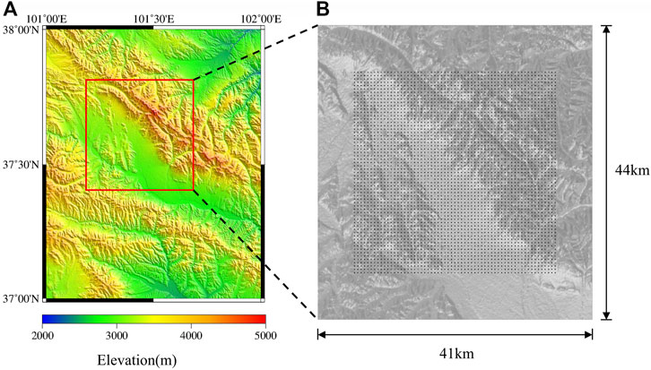
FIGURE 1. (A) Menyuan area elevation map and study region (red box); (B) Locations of the square array of 3,721 virtual receivers (black dots, one station every 500 m).

To isolate topographic site effects from heterogeneities in the subsurface materials, we assume isotropic homogeneous linear elastic half-space with properties given by $V_p=5600$ m/s, $V_s=3354$ m/s, and $\rho =2636$ kg/m³ (Brocher, 2005; Zuo and Chen, 2018). Therefore, the grid size needs to be less than 670 m to simulate ground motion below 5 Hz. The size of the lower grid cell is set to about 620 m, and the size of the upper grid cell is about 210 m, as illustrated in Figure 2A. Two buffer layers (a smoothed version of the surface topography) are introduced to damped mesh distortions of the surface topography (Lee et al., 2008) (Figure 2B). In addition, the mesh between the two buffer layers is refined after balancing the computation cost and accuracy of surface topography modeling.

FIGURE 2

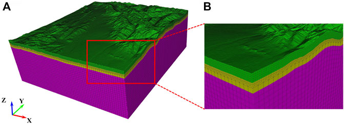
FIGURE 2. (A) Global view of the 3D SEM model; (B) Buffer layer indicate by the red box in (A).

100 Mw 4.5 double couple point sources with Gaussian source time function are used as the input of simulations. The focal mechanisms and locations of each source are randomly generated by uniform distribution, and the rise time is obtained by the empirical scaling relations (Somerville et al., 1999). It should be noted that the rupture area of Mw 4.5 is generally about 2–3 km² (Somerville et al., 1999; Leonard, 2010). The hypocenter depth is limited to above 5 km to ensure the validity of the point source hypothesis. Finding a suitable reference site is not an easy task in the empirical method. But this problem can be easily solved by numerical simulation. An SEM model with a flat ground surface is adopted (the size, medium parameters, and receiver locations of the model are consistent with the previous model) to simulate the reference ground motion. All raw ground motion records in our database need to be filtered by a 4th order Butterworth low-pass filter with a cut-off frequency of 5 Hz before subsequent analysis. Then the three-component ground motion amplification factors of 3,721 receivers can be obtained with the input of each double couple source.

Influence of incident direction on topographic site effects

The amplification factor of PGA, $A{F}_{PGA}$, is defined as the PGA on the topography surface divided by the PGA on the flat ground surface. The data set is divided into 360 subsets based on different back-azimuths (taking $1°$ as the interval), and then the relationship between the mean $A{F}_{PGA}$ of each subset (Abbreviated as $A{F}_{PGA\_BAZ}$) and the back-azimuth is obtained, as shown in Figure 3. The LQT coordinate system is obtained by rotating the XYZ coordinate system based on the specified dipping angle and azimuth, and L, Q, and T represent the polarization directions of P, SV, and SH waves respectively. It can be observed that the $A{F}_{PGA\_BAZ}$ of the T component is consistent with the Y component when the back-azimuth equals to $90°$ or $270°$, and consistent with the X component when the back-azimuth equals to $0°$ ($360°$) or $180°$, which demonstrates that the coordinate rotation is correct.

FIGURE 3

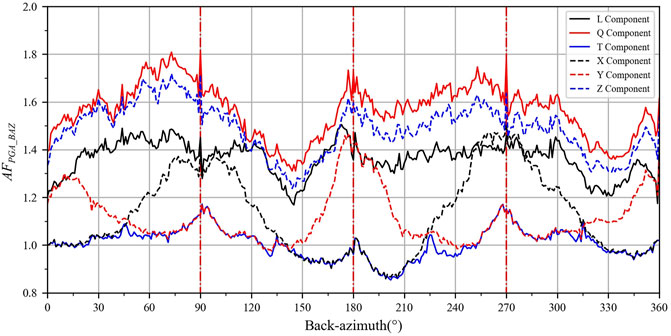
FIGURE 3. The relationship of $A{F}_{PGA\_BAZ}$ with back-azimuth, taking $1°$ as the interval. The solid black, red, and blue lines correspond to the L, Q, and T components, respectively; the dashed black, red, and blue lines correspond to the X, Y, and Z components, respectively. The red vertical dashdot lines are at $0°$ ($360°$), $90°$, $180°$, and $270°$for reference.

For the LQT coordinate system (solid line in Figure 3), the PGA of L and Q components is significantly amplified by the topography, while the $A{F}_{PGA\_BAZ}$ of T component varies around 1.0. The topographic amplification value of SV wave exceeds those of P wave. The curve shapes of L and Q components in Figure 3 are similar, and they both have no obvious correlation with the back-azimuth. For the XYZ coordinate system (dashed line in Figure 3), the $A{F}_{PGA\_BAZ}$ of X component is relatively larger when the back-azimuth is around $90°$ or $270°$; the $A{F}_{PGA\_BAZ}$ of Y component is relatively larger when the back-azimuth is around $0°$ ($360°$) or $180°$. Considering that 80% of the dipping angles in our database are greater than $45°$, the particle motion of P wave is mainly projected on the horizontal plane, resulting in the ground motion amplification of X component (or Y component) being more consistent with that of L component (P wave) in the corresponding back-azimuth. For example, since the topographic amplification of P wave is stronger than that of SH wave, the $A{F}_{PGA}$ of X component will be relatively higher when the particle motion direction of P wave coincides with the X direction (back-azimuth=$90°$ or $270°$), and relatively small when the particle motion direction of SH wave coincides with the X direction (back-azimuth=$0°$ or $180°$).

The maximum $A{F}_{PGA}$ of one receiver with 100 source inputs is defined as $A{F}_{PGA\_\mathit{MAX}}$. The back-azimuths corresponding to the $A{F}_{PGA\_\mathit{MAX}}$ in X, Y, and Z components of all 3,721 receivers is counted, and the density distribution with an interval of $1°$ is shown in Figure 4. The distribution of back-azimuths of the overall database (red solid line) is uniform in the range of $0°$ to $360°$. 41.6% of the $A{F}_{PGA\_\mathit{MAX}}$ in X component occurred in the back-azimuth range of $90°\pm 15°$ and $270°\pm 15°$, 55.1% of the $A{F}_{PGA\_\mathit{MAX}}$ in Y component occurred in the back-azimuth range of $0°\pm 15°$ and $180°\pm 15°$. Compared with Figures 3, 4 further illustrates that the $A{F}_{PGA\_\mathit{MAX}}$ of horizontal components are correlated with the back-azimuth.

FIGURE 4

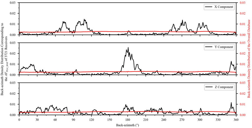
FIGURE 4. The density distribution of back-azimuth. The black solid line represents the density distribution of the back-azimuth corresponding to the $A{F}_{PGA\_\mathit{MAX}}$ of 3,721 receivers (From top to bottom: the X, Y, and Z components, respectively); the solid red line represents the back-azimuth density distribution of the overall database.

The data set is also divided into 90 subsets based on different dipping angles (taking $1°$ as the interval), the mean $A{F}_{PGA}$ of each subset is defined as $A{F}_{PGA\_DIP}$. The influence of dipping angles on $A{F}_{PGA}$ is also shown in Figure 5. As expected, the $A{F}_{PGA\_DIP}$ of Z component in Figure 5A (blue dashed line) is close to that of the L component (black solid line) when dipping angle is equal to $0°$ and close to that of the Q component (red solid line) when the dipping angle is about $80°$. Ding et al. (2017) and Gu et al. (2017) analyzed the seismic ground motion of the scarp topography, and reported that when the slope angle is unchanged, for the inclined P waves, the amplification factor of X component increases, while the amplification factor of Z component decrease with the increase of dipping angle; for the inclined SV waves, the amplification factor of X component decrease, while the amplification factor of Z component increase with the increase of dipping angle. The reason for this phenomenon is also that the increase of the dipping angle will make the P wave project more on the horizontal plane and make the SV wave project more in the vertical direction. It worth noting that topography itself has no influence on dipping angle, but the combination of topographic relief and different dipping angles leads to different forms of ground motion amplification. Due to the amplification of P and SV waves by topography, the $A{F}_{PGA\_DIP}$ of Z component presents a shape of high on both sides and low in the middle. It is worth noting that the double-couple point source and real topographic surface are adopted in this study, so the situation is more complicated than Ding et al. (2017) and Gu et al. (2017).

FIGURE 5

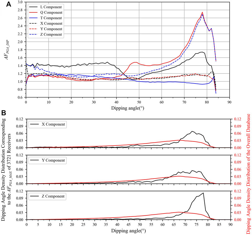
FIGURE 5. The influence of dipping angle on $A{F}_{PGA}$. (A) The relationship of $A{F}_{PGA\_DIP}$ with dipping angle, taking $1°$ as the interval; (B) The density distribution of dipping angle.

The dipping angle density distribution of the overall database is mainly concentrated above 45° (red solid line in Figure 5B), which leads to the particle motion of SV wave is mainly projected in the vertical direction, so the $A{F}_{PGA\_BAZ}$ of Z component is more consistent with that of Q component (SV wave). The $A{F}_{PGA\_BAZ}$ of Z component is greater than that of horizontal components due to that the topographic amplification of SV wave is greater than that of the P and SH waves.

Figure 5B further indicates that the PGA of Z component is strongly amplified when the incident seismic wave is approximately horizontal. For example, 74.5% of the $A{F}_{PGA\_\mathit{MAX}}$ in Z component occurred in the dipping angle range of $75°\pm 5°$, while only 24.8% of the dipping angle in the overall database is in the range of $75°\pm 5°$.

Our simulation data show that the amplification of P and SV waves is independent of back-azimuth, but correlates with dipping angle. Taking the SV wave as an example, when the dipping angle is smaller than $45°$, the $A{F}_{PGA\_DIP}$ of Q component is small; when the dipping angle is larger than $55°$, the $A{F}_{PGA\_DIP}$ of Q component increases with the dipping angle, and reaches the peak when the dipping angle is about $78°$, then decreases rapidly. This phenomenon may be related to the scattering effect of topography, which will be discussed in Discussion section.

Figure 6 represents the density distribution of the dipping angle and the incidence angle, where the incidence angle refers to the angle between the incident direction of seismic wave and the normal to the topography surface at the location of the receiver. The incidence angle in this study is also mainly above 45°, and the relationship between PGA amplification factor and dipping angle is similar to that of the incidence angle, so we will not repeat them here.

FIGURE 6

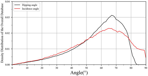
FIGURE 6. Density distribution of dipping angle (black solid line) and incidence angle (red solid line) in the overall database.

Correlation between geomorphometric parameters and topographic site effects

Topographic site effect prediction models based on geomorphometric parameters have been established by previous studies (Maufroy et al., 2015; Zhou et al., 2020). However, due to topographic site effects varying strongly with the stratigraphy and material properties of the underlying geologic material, some researchers believe that topographic site effects cannot be well characterized by studying the effects of ground surface geometry alone (Asimaki and Mohammadi, 2018; Pitarka et al., 2021). Based on the synthetic database, this section studies the correlation between commonly used geomorphometric parameters and topographic amplification to explore whether this correlation can remain stable with different incident directions. The relative elevation and smoothed curvature are initially selected.

Relative elevation ($H_r$) is defined as the difference between the elevation at a point on the surface and the mean elevation within a specified neighborhood of the point. A circular neighborhood with a radius $r$ is used to compute the mean elevation. A positive $H_r$ of a point indicates that the point has a higher elevation relative to the surrounding area, such as the crest; a negative $H_r$ of a point indicates that the point has a lower elevation relative to the surrounding area, such as a valley or the base of a ridge. Note that the value of $H_r$ also depends on the selection of $r$. The $H_r$ is smooth and continuous with the different $r$, and the $H_r$ at a position may both have positive and negative values. The $r$ in this study is set to half of the seismic wavelength, as shown in Eq. 1, where $\lambda$ is the seismic wavelength and the seismic frequency $f$ ranges from 0.4 to 5 Hz with intervals of 0.1 Hz. The minimum value of the frequency range is limited by the size of the model. Our leftmost station is 5500 m from the left boundary of the model. Therefore, the radius we use to calculate the relative elevation cannot exceed 5500 m. Bring it into Eq. 1, and we can get the highest frequency of 0.304 Hz. So we set the lower limit of the frequency range to 0. 4 Hz.The maximum value of the frequency range is limited by the grid division. So we set the upper limit of the frequency range to 5 Hz.The variation range of $r$ in this study is 335.4–4,192.5 m.

$r=\frac{\lambda }{2}=\frac{V_s}{2f}(1)$

Referring to $A{F}_{PGA\_\mathit{MAX}}$, the mean $A{F}_{PGA}$ of one receiver with 100 source inputs is defined as $A{F}_{PGA\_MEAN}$. The Pearson correlation coefficients (Abbreviated as PCC) between $A{F}_{PGA\_MEAN}$ of different components and $H_r$ by varying the radius of surrounding circular area are shown in Figure 7A, in which the $PGA$ of Horizontal component ($PG{A}_{hor}$) and 3D component ($PG{A}_{3D}$) are obtained following Eq. 2, in which $Acc\left(t\right)$ is the acceleration time history of ground motion and the subscripts X, Y and Z indicate the corresponding components respectively.

$\begin{array}{c}PG{A}_{hor}=Maximum\left(\sqrt{Ac{c}_X{\left(t\right)}^2+Ac{c}_Y{\left(t\right)}^2}\right)\\ PG{A}_{3D}=Maximum\left(\sqrt{Ac{c}_X{\left(t\right)}^2+Ac{c}_Y{\left(t\right)}^2+Ac{c}_Z{\left(t\right)}^2}\right)\end{array}(2)$

FIGURE 7

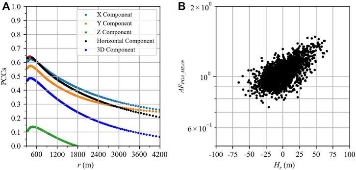
FIGURE 7. Correlation between $A{F}_{PGA\_mean}$ and $H_r$. (A) PCCs of serval components obtained between $H_r$ and $A{F}_{PGA\_MEAN}$; (B) The horizontal $A{F}_{PGA\_MEAN}$ and $H_r$ of the 3,721 receivers indicated by the red dot in (A).

It can be observed from Figure 7A that the PCCs of all components increase first and then decrease with $r$, and $A{F}_{PGA\_MEAN}$ no longer correlate with $H_r$ when $r$ is large to a certain extent, which demonstrates that for a specific site, its topographic site effect ($A{F}_{PGA}$) is affected by the surrounding topographic features within a certain range, but not by the topography at a long distance. The $A{F}_{PGA\_MEAN}$ of X and Y components are found to have a strong correlation with the relative elevation, but not that of Z component. Therefore, the PCC of the horizontal component is greater than that of the 3D component and reaches the peak of 0.64 when $r$ is equal to 400 (red dot in Figure 7A). The increase of $A{F}_{PGA\_MEAN}$ with $H_r$ can be observed in the Figure 7B, which is consistent with our expectation. That is, the amplification of ground motion is easy to occurs near the crest with large $H_r$, while the de-amplification generally occurs near the foot of the hill or valley with small $H_r$.

Wang et al. (2018) also studied the correlation between geomorphometric parameters and PGA amplification. They used the vertically incident plane wave as the input ground motion, without considering the variation of incidence angle. After considering the incidence angle, Figure 7 shows that the correlation is found to be weaker than that of Wang et al. (2018). In addition, Figure 7 also indicates that it is hard to determine the $r$ when $A{F}_{PGA\_MEAN}$ and $H_r$ is best correlated, and the distribution of the scatter points in Figure 7B is quite dispersed, which suggesting that topography-induced PGA amplification cannot be accurately estimated by relying on relative elevation alone.

Topographic amplification is frequency-dependent. The ground motion spectral amplification in this study is defined as $AF\left(f\right)$, which varying with frequency $f$. The Fourier amplitude spectrum $O\left(f\right)$ is obtained by transforming the acceleration time history $Acc\left(t\right)$ from time domain to frequency domain. The amplitude spectra of the horizontal and 3D components are both obtained from the vector amplitudes; that is, $O_{hor}\left(f\right)=\sqrt{O_X{\left(f\right)}^2+O_Y{\left(f\right)}^2}$ and $O_{3D}\left(f\right)=\sqrt{O_X{\left(f\right)}^2+O_Y{\left(f\right)}^2+O_Z{\left(f\right)}^2}$, respectively. Then the spectrum is smoothed by a 0.2 Hz Parzen window. After that$AF\left(f\right)$ can be obtained by dividing the Fourier amplitude spectra of the receiver on the topography surface by the receiver on the flat ground surface.

We calculate the PCCs between $AF\left(f_i\right)$ of 3,721 receivers at the sampling frequency $f_i$ and relative elevation $H_r$ with varying $r$.When $f_i$ is unchanged, each $r$ corresponds to a PCC. All PCCs of $f_i$ can be obtained after traversing all $r$ values, and the relationship between the $r$ value corresponding to the largest PCC and the seismic wavelength $\lambda$ at the $f_i$ is shown in Figure 8A. It is found that when the seismic wavelength is about 2.5 times the $r$, the $AF\left(f\right)$ except for the Z component is best correlated with the $H_r$, and the maximum PCC over different seismic wavelengths is given in Figure 8B. Among all the components, relative elevation $H_r$ has the strongest correlation with $AF\left(f\right)$ of horizontal component and the weakest correlation with $AF\left(f\right)$ of Z component. The PCC between $AF\left(f\right)$ and $H_r$ is larger at low frequency (large wavelength) than at high frequency (small wavelength), and the reason can be attributed to two aspects: the first is the selection of $r$ value. As mentioned earlier, $AF\left(f\right)$ and $H_r$ are most correlated when the wavelength is equal to 2.5 times $r$, but the $r$ is set to half the wavelength [see Eq. 1]. This means that in the high-frequency band, the $r$ corresponding to the maximum PCC will be outside the range of $r$. For example, the wavelength of a 5 Hz seismic wave in this study is 670.8 m, and the $r$ corresponding to the maximum PCC should equal to 670.8/2.5 = 268.32 m, but the minimum value of $r$ is only 335.4 m. Second, the 4th order Butterworth low-pass filter cannot completely filter out the ground motion information above 5 Hz, and the accuracy of numerical simulation may also decline in the high-frequency band.

FIGURE 8

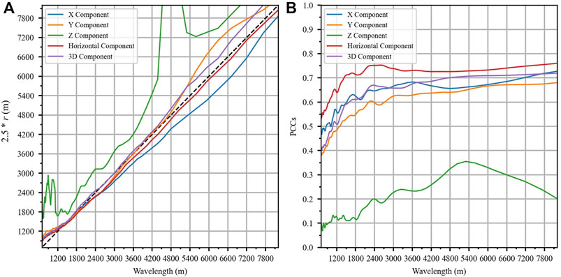
FIGURE 8. The relationship between $AF\left(f\right)$ and $H_r$; (A) The relationship between wavelength and $r$ when $AF\left(f\right)$and $H_r$is best correlated; (B) The maximum PCCs over different seismic wavelengths. Solid lines of different colors in (A) and (B) correspond to different components (see legend in the upper left for details), and the black dashed line in (A) indicates that the value of the abscissa is equal to the ordinate.

By comparing Figure 7A with Figure 8B, we can easily find that $H_r$ has stronger correlation with $AF\left(f\right)$ than that of $A{F}_{PGA}$. We infer that the frequency-dependent topographic amplification is closely related to the scale of topography: large-scale features are correlated to amplification of low-frequency waves, and small-scale features are correlated to amplification of high-frequency waves. $H_r$ with varying $r$ covers topographic feature information in different scales and can better describe $AF\left(f\right)$.

The surface curvature is defined as the second spatial derivative of the elevation map. Following the work of Zevenbergen and Thorne (1987), the Digital Elevation Model (DEM) of the region E should be a rectangular matrix of evenly spaced elevation values with space increment $h$, note that $h$ should be in the same units as the elevations in E (e.g., meters in our study). The curvature at any point $\left(x_i,y_i\right)$ is given by

$\mathit{C}\left(x_i,y_i\right)={\mathit{E}}^{″}\left(x_i,y_i\right)\approx -2\left(\delta +\epsilon \right)\times 100(3)$

In which $\delta$ and $\epsilon$ are second-order derivatives of elevation in x and y components, which are approximated by finite differences as

$\delta =\frac{1}{h^2}\left[\frac{\mathit{E}\left(x_{i-1},y_i\right)+\mathit{E}\left(x_{i+1},y_i\right)}{2}-\mathit{E}\left(x_i,y_i\right)\right](4)$

and

$\epsilon =\frac{1}{h^2}\left[\frac{\mathit{E}\left(x_i,y_{i-1}\right)+\mathit{E}\left(x_i,y_{i+1}\right)}{2}-\mathit{E}\left(x_i,y_i\right)\right](5)$

As shown in Table 1, the PCCs between smoothed curvature and $A{F}_{PGA}$ is low. However, we can find that horizontal PCCs are greater than that of vertical, which means that smoothed curvature also mainly contains information of the horizontal topographic amplification.

TABLE 1

TABLE 1. PCCs between smoothed curvature and $A{F}_{PGA}$.

To characterize the spatial correlation between smoothed curvature and ground-motion amplification as a function of frequency, Maufroy et al. (2015) introduced a smoothing operator, which is to convolve matrix $\mathit{C}$ twice (one per derivative) with a $n\times n$ unit matrix normalized by a factor $n^4$. The smoothed curvature ${\mathit{C}}_s$ is given by

${\mathit{C}}_s=\frac{1}{n^4}\left[\mathit{C}*\left(\begin{array}{ccc}{1}_{11}& \cdots & 1_{1n}\\ ⋮& \ddots & ⋮\\ 1_{n1}& \cdots & 1_{nn}\end{array}\right)*\left(\begin{array}{ccc}{1}_{11}& \cdots & 1_{1n}\\ ⋮& \ddots & ⋮\\ 1_{n1}& \cdots & 1_{nn}\end{array}\right)\right](6)$

The characteristic length is defined as $L_s=2\times n\times h$. According to Maufroy et al. (2015), the highest correlation between frequency-dependent topographic amplification and the smoothed curvature is reached when the curvature is smoothed over a characteristic length equal to half of the S wavelength, which is also confirmed in Figure 9A. In addition, Figures 7–9 show that the geomorphometric parameters have the best correlation with the horizontal topographic amplification and the worst in the vertical component.

FIGURE 9

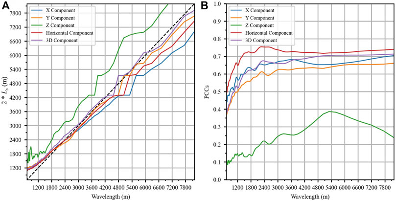
FIGURE 9. The relationship between $AF\left(f\right)$ and $C_s$; (A) The relationship between wavelength and $L_s$ when $AF\left(f\right)$and ${\mathit{C}}_s$is best correlated; (B) The maximum PCCs over different seismic wavelengths. Solid lines of different colors in (A,B) correspond to different components (see legend in the upper left for details), and black dashed line in (A) indicates that the value of the abscissa is equal to the ordinate.

Based on the above analysis, it is easy to notice the strong similarity between relative elevation $H_r$ and smoothed curvature ${\mathit{C}}_s$. Rai et al. (2016) demonstrated that $H_r$ and ${\mathit{C}}_s$ are highly correlated. Wang et al. (2018) took Hong Kong Island as a local testbed site and used a square neighborhood with the length defined as $L_h$ to calculate $H_r$. They found that the best correlation between $H_r$ and ${\mathit{C}}_s$ is obtained when $L_h=1.5\times L_s$ and the corresponding coefficient of determination R² is as high as 0.94. Based on the DEM of this study, the relationship between relative elevation and smooth curvature is analyzed. As shown in Figure 10, the R² between $H_r$ and ${\mathit{C}}_s$ in this study is as high as 0.975 when $L_s=1.25r$. Considering that a circular area of radius $r$ is used in this study, Figure 10 is consistent with Wang et al. (2018). In addition, Figure 10 further indicates that the strong correlation between $H_r$ and ${\mathit{C}}_s$ is not limited by the study area, which means that relative elevation and smooth curvature with given length scales represent the same information of the topography. The initially acquired surface topography data is usually unprocessed digital elevation data, and considering the algorithmic complexity, relative elevation $H_r$ is recommended as a proxy for topographic site effects.

FIGURE 10

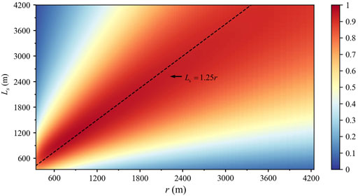
FIGURE 10. Coefficients of determination between relative elevation and smoothed curvature with various $r$ and $L_s$.

Discussion

The influence of the incident direction of seismic waves on the topographic site effect is revealed in this work based on a large number of 3D numerical simulations, which is useful for us to explain the spatial distribution characteristics of ground motion. However, the applicability of these findings in real earthquake scenarios needs to be discussed.

The homogeneous velocity model introduced in this study leads to some discrepancies between the numerical simulation results and the real earthquake cases, one of which is the difference in dipping angle. In real earthquake scenarios, the shear velocity increase with depth whether it is homogeneous rock or unconsolidated sediments (Kanamori and Schubert, 2015). Based on Snell’s law, when the seismic wave is transmitted from the larger shear velocity medium to the smaller shear velocity medium, the direction of the refracted wave will approach the normal direction. Even if the initial dipping angle is very large, the propagating path of the seismic wave will become approximately vertical in the near-surface after several refractions. Since seismic waves do not refract in the medium with uniform shear velocity (e.g., numerical models used in this work), the dipping angle of seismic waves at the ground surface will be much larger than that in the real world. Based on the discussion of Figure 5 above, the larger dipping angle is part of the reason why the $A{F}_{PGA}$ of vertical component is greater than that of the horizontal components, while investigation of historical earthquakes generally shows that topography has a much larger ground motion amplification effect on the horizontal components than on the vertical component. The relationship between back-azimuth and the strength of topographic amplification should be available at bedrock sites [such as Classes A in NEHRP (National Earthquake Hazards Reduction Program) Site Classification] under shallow earthquakes with large hypocenter distances (The point source assumptions). While the point source assumption is not met, there is not a clear relationship between the back-azimuth and the degree of amplification (e.g., Stone et al., 2022).

Numerical simulations and model experiment show that the scattering of body waves to surface waves can be induced by topographic features in homogeneous linear elastic half-space (Gangi and Wesson, 1978; Boore et al., 1981; Ohtsuki and Harumi, 1983; Li and Liao, 2002). We also confirm the existence of converted surface wave based on the spectral element method, see Supplementary Material document for details. The dipping angle may be related to the strength of the generated surface wave. Li and Liao (2002) indicates that the top corner of cliff scatter stronger Rayleigh wave under inclined body waves than vertical body waves and the maximum amplitude of converted Rayleigh wave is about 1.1 times of the free field surface displacement. Assimaki et al. (2005a) demonstrated that all the incident energy with the critical incidence angle (i.e., $\arcsin \left(\raisebox{1ex}{$V_S$}\!\left/ \!\raisebox{-1ex}{$V_P$}\right.\right)$ for Poisson’s ratio of the elastic medium is 0.35) practically transforms into surface waves. Tsai et al. (2017) and Kang et al. (2019) also indicated that large incidence angles increase the possibility of surface wave generation. We speculate that the increase of dipping angle will strengthen the converted surface wave, and then the constructive interference between the generated surface wave and the direct SV wave results in the strong amplification of L and Q components. Since the total energy remains unchanged, the amplification factors of T component become decrease.

Although numerical simulations alone are not as powerful as simulations used in conjunction with real data, it is currently one of the best ways to understand the mechanisms of topographic site effects. The role of different factors in controlling the highly variable amplification effects is unclear, and the numerical simulation methods are very flexible and can solve these problems to a certain extent. Previous studies have built appropriate models according to the research targets to study the influence of a specific factor on the ground motion (e.g., Lee et al., 2009a; Lee et al., 2009b). It is difficult to explore the influence of back-azimuth on topographic site effect based on real data. The challenges are mainly manifested in two aspects: the first is there are many limitations when selecting a reference station, which is related to the reliability of the topographic amplification factors. The second is that there should be enough historical ground motion records. To ensure the robustness of the conclusion, at least one or two historical earthquakes are required in every $1°$ back-azimuth. However, with the construction of stations and the increase of observation records, our conclusions are expected to be verified in the future.

We found that the relative elevation is indeed closely related to the horizontal ground motion amplification, but even for the idealized numerical model used in this paper, this correlation still shows a certain discreteness, which imposes a challenge to the accuracy of the GMM; on the other hand, post-earthquake disaster assessment generally focuses on specific sites that including both muti-layer subsurface structures and topographic features, which imposes a challenge to the applicability of the GMM. Therefore, we plan to classify the topographic features based on the geomorphometric parameters, and then combine it with the site classification (e.g., NEHRP site classification) to evaluate the ground motion amplification level in the real engineering site.

Conclusion

In this paper, we study the influence of back-azimuth and dipping angle on the topographic amplification based on the ground motion synthetic database constructed by the spectral element method. In addition, the correlation between geomorphometric parameters (relative elevation and smooth curvature) and frequency-dependent topographic amplification value is also analyzed. For the isotropic homogeneous numerical model with double couple point sources as the input, the following conclusions can be obtained:

(1) When the dipping angle is smaller than $45°$, topography has a strong amplification effect on P waves; When the dipping angle is greater than $45°$, topography has a strong amplification effect on SV wave, followed by P wave, and it has the least amplification effect on SH wave.

(2) When the dipping angle is large, the topographic amplification of P wave is more projected on the horizontal components. More specifically, When the back-azimuth angle is around 90° or 270°, the PGA amplification of the X component increases obviously; when the back-azimuth is around 0° or 180°, the PGA amplification of the Y component increases obviously. The PGA amplification of Z component is independent of the back-azimuth and similar to that of SV wave.

(3) The relative elevation and smoothed curvature cover the same information of topography, Considering the algorithmic complexity, relative elevation is recommended as a proxy for topographic site effects.

(4) The correlation of geomorphometric parameters (relative elevation and smoothed curvature) with spectral amplification is stronger than that of geomorphometric parameters with PGA amplification.

(5) The relative elevation and smoothed curvature are both closely related to the horizontal topographic amplification, but independent of that in the vertical component.

Data availability statement

The original contributions presented in the study are included in the article/Supplementary Material, further inquiries can be directed to the corresponding author.

Author contributions

FW implemented the numerical simulations and specifically writing the initial draft. QM determined the research goals and contributed to designing the methodology. DT and QX provided important suggestions for the interpretation of the results and revised the manuscript. All authors contributed to the redaction and final revision of the manuscript.

Funding

This research was partially supported by Scientific Research Fund of Institute of Engineering Mechanics, China Earthquake Administration (Grant No. 2016A03), and National Natural Science Foundation of China (Grant No. U2039209 and 5150082083).

Acknowledgments

We thank NASA’s (National Aeronautics and Space Administration) EOSDIS (Earth Observing System Data and Information System) (https://search.earthdata.nasa.gov) for providing DEM (Digital Elevation Model) data. Some plots were made using Generic Mapping Tools v.5.2.1 and the matplotlib module in Python.

Conflict of interest

The authors declare that the research was conducted in the absence of any commercial or financial relationships that could be construed as a potential conflict of interest.

Publisher’s note

All claims expressed in this article are solely those of the authors and do not necessarily represent those of their affiliated organizations, or those of the publisher, the editors and the reviewers. Any product that may be evaluated in this article, or claim that may be made by its manufacturer, is not guaranteed or endorsed by the publisher.

Supplementary material

The Supplementary Material for this article can be found online at: https://www.frontiersin.org/articles/10.3389/feart.2022.996389/full#supplementary-material

SUPPLEMENTARY TABLES S1–S2 | Show the coordinate positions of seismic events and stations in the numerical model, respectively.

References

Ashford, S. A., and Sitar, N. (1997). Analysis of topographic amplification of inclined shear waves in a steep coastal bluff. Bull. Seismol. Soc. Am. 87, 692–700. doi:10.1785/BSSA0870030692

CrossRef Full Text | Google Scholar

Asimaki, D., and Mohammadi, K. (2018). On the complexity of seismic waves trapped in irregular topographies. Soil Dyn. Earthq. Eng. 114, 424–437. doi:10.1016/j.soildyn.2018.07.020

CrossRef Full Text | Google Scholar

Assimaki, D., Gazetas, G., and Kausel, E. (2005a). Effects of local soil conditions on the topographic aggravation of seismic motion: Parametric investigation and recorded field evidence from the 1999 athens earthquake. Bull. Seismol. Soc. Am. 95, 1059–1089. doi:10.1785/0120040055

CrossRef Full Text | Google Scholar

Assimaki, D., and Gazetas, G. (2004). Soil and topographic amplification on canyon banks and the 1999 Athens earthquake. J. Earth. Eng. 8, 1–43. doi:10.1142/S1363246904001250

CrossRef Full Text | Google Scholar

Assimaki, D., Kausel, E., and Gazetas, G. (2005b). Soil-dependent topographic effects: A case study from the 1999 athens earthquake. Earthq. Spectra 21, 929–966. doi:10.1193/1.2068135

CrossRef Full Text | Google Scholar

Boore, D. M. (1972). A note on the effect of simple topography on seismic SH waves. Bull. Seismol. Soc. Am. 62, 275–284. doi:10.1785/BSSA0620010275

CrossRef Full Text | Google Scholar

Boore, D. M., Harmsen, S. C., and Harding, S. T. (1981). Wave scattering from a step change in surface topography. Bull. Seismol. Soc. Am. 71, 117–125. doi:10.1785/BSSA0710010117

CrossRef Full Text | Google Scholar

Borcherdt, R. D. (1970). Effects of local geology on ground motion near San Francisco Bay. Bull. Seismol. Soc. Am. 60, 29–61. doi:10.1785/BSSA0600010029

CrossRef Full Text | Google Scholar

Bouchon, M., and Barker, J. S. (1996). Seismic response of a hill: The example of Tarzana, California. Bull. Seismol. Soc. Am. 86, 66–72. doi:10.1785/BSSA08601A0066

CrossRef Full Text | Google Scholar

Bouckovalas, G. D., and Papadimitriou, A. G. (2005). Numerical evaluation of slope topography effects on seismic ground motion. Soil Dyn. Earthq. Eng. 25, 547–558. doi:10.1016/j.soildyn.2004.11.008

CrossRef Full Text | Google Scholar

Brocher, T. M. (2005). Empirical relations between elastic wavespeeds and density in the earth's crust. Bull. Seismol. Soc. Am. 95, 2081–2092. doi:10.1785/0120050077

CrossRef Full Text | Google Scholar

Buech, F., Davies, T., and Pettinga, J. (2010). The little red hill seismic experimental study: Topographic effects on ground motion at a bedrock-dominated mountain edifice. Bull. Seismol. Soc. Am. 100, 2219–2229. doi:10.1785/0120090345

CrossRef Full Text | Google Scholar

Burjánek, J., Edwards, B., and Fäh, D. (2014). Empirical evidence of local seismic effects at sites with pronounced topography: A systematic approach. Geophys. J. Int. 197, 608–619. doi:10.1093/gji/ggu014

CrossRef Full Text | Google Scholar

Burjánek, J., Moore, J. R., Yugsi Molina, F. X., and Fäh, D. (2012). Instrumental evidence of normal mode rock slope vibration. Geophys. J. Int. 188, 559–569. doi:10.1111/j.1365-246X.2011.05272.x

CrossRef Full Text | Google Scholar

Ding, H., Yu, Y., and Zheng, Z. (2017). Effects of scarp topography on seismic ground motion under inclined P waves. Rock Soil Mech. 38, 1716–1724+1732. doi:10.16285/j.rsm.2017.06.021

CrossRef Full Text | Google Scholar

Galvez, P., Petukhin, A., Somerville, P., Ampuero, J. P., Miyakoshi, K., Peter, D., et al. (2021). Multicycle simulation of strike-slip earthquake rupture for use in near-source ground-motion simulations. Bull. Seismol. Soc. Am. 111, 2463–2485. doi:10.1785/0120210104

CrossRef Full Text | Google Scholar

Gangi, A. F., and Wesson, R. L. (1978). P-wave to Rayleigh-wave conversion coefficients for wedge corners; model experiments. J. Comput. Phys. 29, 370–388. doi:10.1016/0021-9991(78)90140-7

CrossRef Full Text | Google Scholar

Geli, L., Bard, P.-Y., and Jullien, B. (1988). The effect of topography on earthquake ground motion: A review and new results. Bull. Seismol. Soc. Am. 78, 42–63. doi:10.1785/BSSA0780010042

CrossRef Full Text | Google Scholar

Gu, L., Ding, H., and Yu, Y. (2017). Effects of scarp topography on seismic ground motion under inclined SV waves. J. Nat. Disast. 26, 39–47. doi:10.13577/j.jnd.2017.0405

CrossRef Full Text | Google Scholar

Harris, R. A. (1998). Forecasts of the 1989 loma prieta, California, earthquake. Bull. Seismol. Soc. Am. 88, 898–916. doi:10.1785/BSSA0880040898

CrossRef Full Text | Google Scholar

Hartzell, S. H., Carver, D. L., and King, K. W. (1994). Initial investigation of site and topographic effects at Robinwood Ridge, California. Bull. Seismol. Soc. Am. 84, 1336–1349. doi:10.1785/BSSA0840051336

CrossRef Full Text | Google Scholar

Hartzell, S., Ramírez-Guzmán, L., Meremonte, M., and Leeds, A. (2017). Ground motion in the presence of complex topography II: Earthquake sources and 3D simulations. Bull. Seismol. Soc. Am. 107, 344–358. doi:10.1785/0120160159

CrossRef Full Text | Google Scholar

Hough, S. E., Altidor, J. R., Anglade, D., Given, D., Janvier, M. G., Maharrey, J. Z., et al. (2010). Localized damage caused by topographic amplification during the 2010 M 7.0 Haiti earthquake. Nat. Geosci. 3, 778–782. doi:10.1038/ngeo988

CrossRef Full Text | Google Scholar

Igel, H. (2017). Computational seismology: A practical introduction. Oxford, United Kingdom: Oxford University Press.

Google Scholar

Kanamori, H., and Schubert, G. (2015). Treatise on geophysics: Earthquake seismology. Amsterdam, Netherlands: Elsevier Press.

Google Scholar

Kang, S., Kim, B., Cho, H., Lee, J., Kim, K., Bae, S., et al. (2019). Ground-motion amplifications in small-size hills: Case study of gokgang-ri, South Korea, during the 2017 M_L 5.4 pohang earthquake sequence. Bull. Seismol. Soc. Am. 109, 2626–2643. doi:10.1785/0120190064

CrossRef Full Text | Google Scholar

Komatitsch, D., Tsuboi, S., Tromp, J., Levander, A., and Nolet, G. (2005). The spectral-element method in seismology. Geoph. Mono. Am. Geoph.Un. 157, 205.

Google Scholar

La Rocca, M., Chiappetta, G. D., Gervasi, A., and Festa, R. L. (2020). Non-stability of the noise HVSR at sites near or on topographic heights. Geophys. J. Int. 222, 2162–2171. doi:10.1093/gji/ggaa297

CrossRef Full Text | Google Scholar

Lee, S.-J., Chan, Y.-C., Komatitsch, D., Huang, B.-S., and Tromp, J. (2009a). Effects of realistic surface topography on seismic ground motion in the Yangminshan region of Taiwan based upon the Spectral-Element Method and LiDAR DTM. Bull. Seismol. Soc. Am. 99, 681–693. doi:10.1785/0120080264

CrossRef Full Text | Google Scholar

Lee, S.-J., Chen, H.-W., Liu, Q., Komatitsch, D., Huang, B.-S., and Tromp, J. (2008). Three-dimensional simulations of seismic-wave propagation in the Taipei Basin with realistic topography based upon the spectral-element method. Bull. Seismol. Soc. Am. 98, 253–264. doi:10.1785/0120070033

CrossRef Full Text | Google Scholar

Lee, S.-J., Komatitsch, D., Huang, B.-S., and Tromp, J. (2009b). Effects of topography on seismic-wave propagation: An example from northern Taiwan. Bull. Seismol. Soc. Am. 99, 314–325. doi:10.1785/0120080020

CrossRef Full Text | Google Scholar

Leonard, M. (2010). Earthquake fault scaling: Self-consistent relating of rupture length, width, average displacement, and moment release. Bull. Seismol. Soc. Am. 100, 1971–1988. doi:10.1785/0120090189

CrossRef Full Text | Google Scholar

Li, S. Y., and Liao, Z. P. (2002). Wave-type conversion caused by a step topography subjected to inclined seismic body wave. Earthq. Eng. Eng. Vib. 22, 9–15. doi:10.13197/j.eeev.2002.04.002

CrossRef Full Text | Google Scholar

Lovati, S., Bakavoli, M. K. H., Massa, M., Ferretti, G., Pacor, F., Paolucci, R., et al. (2011). Estimation of topographical effects at Narni ridge (Central Italy): Comparisons between experimental results and numerical modelling. Bull. Earthq. Eng. 9, 1987–2005. doi:10.1007/s10518-011-9315-x

CrossRef Full Text | Google Scholar

Luo, Y., Del Gaudio, V., Huang, R., Wang, Y., and Wasowski, J. (2014). Evidence of hillslope directional amplification from accelerometer recordings at qiaozhuang (sichuan — China). Eng. Geol. 183, 193–207. doi:10.1016/j.enggeo.2014.10.015

CrossRef Full Text | Google Scholar

Luo, Y., Fan, X., Huang, R., Wang, Y., Yunus, A. P., and Havenith, H.-B. (2020). Topographic and near-surface stratigraphic amplification of the seismic response of a mountain slope revealed by field monitoring and numerical simulations. Eng. Geol. 271, 105607. doi:10.1016/j.enggeo.2020.105607

CrossRef Full Text | Google Scholar

Ma, Q., Wang, F., Tao, D., Xie, Q., Liu, H., and Jiang, P. (2021). Topographic site effects of Xishan Park ridge in Zigong city, Sichuan considering epicentral distance. J. Seismol. 25, 1537–1555. doi:10.1007/s10950-021-10048-7

CrossRef Full Text | Google Scholar

Magnoni, F., Casarotti, E., Michelini, A., Piersanti, A., Komatitsch, D., Peter, D., et al. (2013). Spectral-Element simulations of seismic waves generated by the 2009 L’Aquila earthquake. Bull. Seismol. Soc. Am. 104, 73–94. doi:10.1785/0120130106

CrossRef Full Text | Google Scholar

Maufroy, E., Cruz-Atienza, V. M., Cotton, F., and Gaffet, S. (2015). Frequency-Scaled curvature as a proxy for topographic site-effect amplification and ground-motion variability. Bull. Seismol. Soc. Am. 105, 354–367. doi:10.1785/0120140089

CrossRef Full Text | Google Scholar

Mayoral, J. M., De la Rosa, D., and Tepalcapa, S. (2019). Topographic effects during the September 19, 2017 Mexico city earthquake. Soil Dyn. Earthq. Eng. 125, 105732. doi:10.1016/j.soildyn.2019.105732

CrossRef Full Text | Google Scholar

Moore, J. R., Gischig, V., Burjanek, J., Loew, S., and Fäh, D. (2011). Site effects in unstable rock slopes: Dynamic behavior of the Randa instability (Switzerland). Bull. Seismol. Soc. Am. 101, 3110–3116. doi:10.1785/0120110127

CrossRef Full Text | Google Scholar

Nakamura, Y. (1989). A method for dynamic characteristics estimation of subsurface using microtremor on the ground surface. Q. Rep. Railw. Tech. Res. Inst. 30, 25–33.

Google Scholar

Ohtsuki, A., and Harumi, K. (1983). Effect of topography and subsurface inhomogeneities on seismic SV waves. Earthq. Eng. Struct. Dyn. 11, 441–462. doi:10.1002/eqe.4290110402

CrossRef Full Text | Google Scholar

Paolucci, R. (2002). Amplification of earthquake ground motion by steep topographic irregularities. Earthq. Eng. Struct. Dyn. 31, 1831–1853. doi:10.1002/eqe.192

CrossRef Full Text | Google Scholar

Pischiutta, M., Cultrera, G., Caserta, A., Luzi, L., and Rovelli, A. (2010). Topographic effects on the hill of Nocera Umbra, central Italy. Geophys. J. Int. 182, 977–987. doi:10.1111/j.1365-246X.2010.04654.x

CrossRef Full Text | Google Scholar

Pitarka, A., Akinci, A., De Gori, P., and Buttinelli, M. (2021). Deterministic 3D ground-motion simulations (0–5 Hz) and surface topography effects of the 30 October 2016 Mw 6.5 Norcia, Italy, earthquake. Bull. Seismol. Soc. Am. 112, 262–286. doi:10.1785/0120210133

CrossRef Full Text | Google Scholar

Rai, M., Rodriguez-Marek, A., and Yong, A. (2016). An empirical model to predict topographic effects in strong ground motion using California small- to medium-magnitude earthquake database. Earthq. Spectra 32, 1033–1054. doi:10.1193/113014eqs202m

CrossRef Full Text | Google Scholar

Somerville, P., Irikura, K., Graves, R., Sawada, S., Wald, D., Abrahamson, N., et al. (1999). Characterizing crustal earthquake slip models for the prediction of strong ground motion. Seismol. Res. Lett. 70, 59–80. doi:10.1785/gssrl.70.1.59

CrossRef Full Text | Google Scholar

Song, J., Gao, Y., and Feng, T. (2020). Influence of interactions between topographic and soil layer amplification on seismic response of sliding mass and slope displacement. Soil Dyn. Earthq. Eng. 129, 105901. doi:10.1016/j.soildyn.2019.105901

CrossRef Full Text | Google Scholar

Stolte, A. C., Cox, B. R., and Lee, R. C. (2017). An experimental topographic amplification study at Los Alamos National Laboratory using ambient vibrations. Bull. Seismol. Soc. Am. 107, 1386–1401. doi:10.1785/0120160269

CrossRef Full Text | Google Scholar

Stone, I., Wirth, E. A., and Frankel, A. D. (2022). Topographic response to simulated Mw 6.5–7.0 earthquakes on the seattle fault. Bull. Seismol. Soc. Am. 112, 1436–1462. doi:10.1785/0120210269

CrossRef Full Text | Google Scholar

Trifunac, M. D., and Hudson, D. E. (1971). Analysis of the Pacoima Dam accelerogram-san Fernando, California, earthquake of 1971. Bull. Seismol. Soc. Am. 61, 1393–1141. doi:10.1785/BSSA0610051393

CrossRef Full Text | Google Scholar

Tsai, V. C., Bowden, D. C., and Kanamori, H. (2017). Explaining extreme ground motion in Osaka basin during the 2011 Tohoku earthquake. Geophys. Res. Lett. 44, 7239–7244. doi:10.1002/2017GL074120

CrossRef Full Text | Google Scholar

Tucker, B. E., King, J. L., Hatzfeld, D., and Nersesov, I. L. (1984). Observations of hard-rock site effects. Bull. Seismol. Soc. Am. 74, 121–136. doi:10.1785/BSSA0740010121

CrossRef Full Text | Google Scholar

Wang, G., Du, C., Huang, D., Jin, F., Roo, R. C. H., and Kwan, J. S. H. (2018). Parametric models for 3D topographic amplification of ground motions considering subsurface soils. Soil Dyn. Earthq. Eng. 115, 41–54. doi:10.1016/j.soildyn.2018.07.018

CrossRef Full Text | Google Scholar

Wang, L., Wu, Z., Xia, K., Liu, K., Wang, P., Pu, X., et al. (2019). Amplification of thickness and topography of loess deposit on seismic ground motion and its seismic design methods. Soil Dyn. Earthq. Eng. 126, 105090. doi:10.1016/j.soildyn.2018.02.021

CrossRef Full Text | Google Scholar

Wang, X., Wang, J., Zhang, L., and He, C. (2021). Broadband ground-motion simulations by coupling regional velocity structures with the geophysical information of specific sites. Soil Dyn. Earthq. Eng. 145, 106695. doi:10.1016/j.soildyn.2021.106695

CrossRef Full Text | Google Scholar

Wood, C. M., and Cox, B. R. (2016). Comparison of field data processing methods for the evaluation of topographic effects. Earthq. Spectra 32, 2127–2147. doi:10.1193/111515eqs170m

CrossRef Full Text | Google Scholar

Yuan, X., and Liao, Z. (1996). Scattering of plane SH waves by arbitrary circular convex topography. Earthq. Eng. Eng. Vib. 16, 1–13. doi:10.13197/j.eeev.1996.02.001

CrossRef Full Text | Google Scholar

Yuan, Y. O., Lacasse, M. D., and Liu, F. (2021). Full-wavefield, full-domain deterministic modeling of shallow low-magnitude events for improving regional ground-motion predictions. Bull. Seismol. Soc. Am. 111, 2617–2634. doi:10.1785/0120210031

CrossRef Full Text | Google Scholar

Zevenbergen, L. W., and Thorne, C. R. (1987). Quantitative analysis of land surface topography. Earth Surf. Process. Landf. 12, 47–56. doi:10.1002/esp.3290120107

CrossRef Full Text | Google Scholar

Zhou, H., Li, J., and Chen, X. (2020). Establishment of a seismic topographic effect prediction model in the Lushan Ms 7.0 earthquake area. Geophys. J. Int. 221, 273–288. doi:10.1093/gji/ggaa003

CrossRef Full Text | Google Scholar

Zuo, K., and Chen, J. (2018). 3D body-wave velocity structure of crust and relocation of earthquakes in the Menyuan area. Chin. J. Geophys. 61, 2788–2801. doi:10.6038/cjg2018L0537

CrossRef Full Text | Google Scholar