 Jinmeng Bi
 Fengling Yin
 Changsheng Jiang
 Xinxin Yin1,3
95% of researchers rate our articles as excellent or good
Learn more about the work of our research integrity team to safeguard the quality of each article we publish.
Find out more
ORIGINAL RESEARCH article
Front. Earth Sci. , 16 January 2023
Sec. Solid Earth Geophysics
Volume 10 - 2022 | https://doi.org/10.3389/feart.2022.994850
This article is part of the Research Topic From Preparation to Faulting: Multidisciplinary Investigations on Earthquake Processes View all 12 articles
Strong aftershocks, especially the disaster-causing M≥5.0 kind, are a key concern for mitigation of seismic risks because they often lead to superimposed earthquake damage. However, the real-time forecasting results of the traditional probability prediction models based on statistics are usually far from accurate and therefore unsatisfactory. Borrowing an idea from the foreshock traffic light system (FTLS), which is based on observations of decreasing b-values or increasing differential stress just before a strong aftershock, we constructed a strong aftershock traffic light system (SATLS) that uses data-driven technology to improve the reliability of time sequence b-value calculations, and analyzed the b-value variations of strong aftershocks in the China continent. We applied this system to the MS6.9 Menyuan earthquake occurred on 8 January 2022. The earthquake occurrence rates before the largest aftershock (MS5.2) forecast by the Omi-R-J model were too low, although the model could accurately forecast aftershock rates for each magnitude interval in most time-periods. However, reliable b-values can be calculated using the time-sequence b-value data-driven (TbDD) method, and the results showed that the b-values continued declining from 1.3 days before the MS5.2 aftershock and gradually recovered afterward. This would suggest that the stress evolution in the focal area can provide data for deciding when to post risk alerts of strong aftershocks. In the process of building the SATLS, we studied thirty-four M≥6.0 intraplate earthquake sequences in the China continent and concluded that the differences between the b-values of the aftershock sequences and of the background events, △b = bafter - bbg = ±0.1, could be used as thresholds to determine whether M≥5.0 aftershocks would occur. The △b value obtained using the events before the MS5.2 aftershock of the MS6.9 Menyuan sequence was about -0.04, which would have caused the SATLS to declare a yellow alert, but there would have been some gap expected before a red alert was triggered by the b-value difference derived from the events associated with this strong aftershock. To accurately forecast a strong aftershock of M≥5.0, a deeper understanding of the true b-value and a detailed description of the stress evolution state in the source area is necessary.
The disastrous effects of superimposed strong aftershocks on buildings and structures have aggravated casualties and property losses, such as occurred in the M7.1 Luanxian strong aftershock and the M6.9 Ninghe strong aftershock after the 1976 M7.8 Tangshan earthquake (Lv et al., 2007) and the strong M6.3 aftershock after the 2010 M7.1 earthquake in New Zealand (Zhang et al., 2011). Accurate and reliable forecasting of strong aftershocks is of great importance to post-earthquake emergency evacuation, secondary disaster disposal, and decision-making for restoration and reconstruction (Woessner et al., 2011; Nanjo et al., 2012; Ogata et al., 2013). Traditional strong aftershock forecasting, which is realized mainly by short-term probability forecasting models (Jiang et al., 2018; Bi et al., 2020; Bi and Jiang, 2020) such as the Reasenberg–Jones (R-J) model (Reasenberg and Jones, 1989), the epidemic-type aftershock sequence (ETAS) model (Ogata, 1989), and the Omi-R-J model (Omi et al., 2013, 2015, 2016), still faces great challenges in real-time functionality and accuracy (Lippiello et al., 2017). For example, the Japan Meteorological Agency (JMA) announced a low-probability forecast of M≥5.5 aftershocks for the 2005 M7.0 earthquake off the coast of western Fukuoka Prefecture, Kyushu District, Japan; but, in fact, the earthquake was followed by the largest aftershock of M5.8 (Ogata, 2006). In addition, using only the ETAS model to predict the frequency of strong aftershocks in Japan and Southern California (Grimm et al., 2021) and the largest expected aftershock of the 2019 Ridgecrest earthquake sequence in the United States (Shcherbakov, 2021) revealed the model’s obvious shortcomings.
In recent years, a new route for the development of strong aftershock forecasting technology has employed the concept of graded risk assessment to improve the operability of forecasting based on abnormal aftershock activity (Matsu’ura, 1986; Ogata, 2001). Gulia and Wiemer (2019) proposed the foreshock traffic light system (FTLS), which uses b-values that are sensitive to stress changes, and achieved good results in earthquake cases studies. The theoretical basis of FTLS posits that the b-value in relation to G-R can be used as an indirect description of underground differential stress (Gutenberg and Richter, 1944; Scholz, 1968; Scholz, 2015), and that the change in b-value is related to the state of underground stress load (Chan and Chandler, 2001; Nandan et al., 2017; Si and Jiang, 2019); some earthquake cases studies showed that the b-value can increase by 20% after the main shock and decrease by 10% or more before the strong aftershock (Gulia et al., 2018; Gulia and Wiemer, 2019). Nanjo et al. (2022) further improved FTLS by combining local aseismic slips with stress changes. In addition, the idea of a risk classification traffic light system was also widely applied in research of induced earthquake risk control (Jiang et al., 2021b), aftershock hazard analysis (Gulia et al., 2020), and risk assessment of cumulative structural damage caused by aftershocks (Trevlopoulos et al., 2020). However, there is still room for further development in the technical route of strong aftershock forecasting. This can be accomplished through improvements in the risk classification method by an empirical understanding that the b-value change of aftershocks compared to that before the earthquake is universal in different tectonic regions and an increased awareness of the influence of subjectivity in the calculation of time series b-values (Jiang et al., 2021a; Jiang et al., 2021).
On 8 January 2022, an MS6.9 earthquake struck Menyuan County, Qinghai Province, northwestern China, and ruptured the Tuolaishan fault (TLSF) and the Lenglongling fault (LLLF) for about 415 km. It affected nearly 6,000 people, damaged more than 4,000 homes and buildings, and caused a large number of secondary disasters such as local slope collapse, rolling stones, cracking of frozen soil, and arch deformation of ice surfaces (https://m.gmw.cn/baijia/2022-01/20/35460649.html). Two strong aftershocks of MS5.1 and MS5.2 occurred on January 8 and January 12, respectively, and the latter caused the aftershock area to extend more than 10 km toward the southeast, which was close to the aftershock area of the 2016 MS6.4 Menyuan earthquake. This phenomenon brought widespread concerns about the strong aftershock risk of the 2022 MS6.9 Menyuan earthquake. To investigate this risk, we first carried out quantitative aftershock probability forecasting and analyzed the forecasting effectiveness. Second, based on cases studies of the time evolution of b-values of intraplate earthquake sequences in the China continent and the occurrence regularity of strong aftershocks, we constructed a strong aftershock traffic light system (SATLS), which is more universal than the FTLS, to qualitatively evaluate the risk of strong aftershocks after the 2022 MS6.9 Menyuan earthquake. This study provides a scientific basis for improving the forecasting of strong aftershocks following similar complex earthquake sequences.
We used the Omi-R-J model (Omi et al., 2013) to conduct aftershock probability forecasting for the MS6.9 Menyuan earthquake sequence and evaluated the performance of this forecasting method. The Omi-R-J model, which combines the traditional R-J model (Reasenberg and Jones, 1989) with the OK1993 model (Ogata and Katsura, 1993) describing the magnitude–frequency relationship in the form of a continuous function, can make full use of a large number of small earthquakes below the completeness magnitude in the early stages of an earthquake sequence and produce relatively reliable and stable results in terms of parameter fitting to the model and forecasting of the aftershock occurrence rate. Under the conditions of a non-cumulative magnitude–frequency distribution, the OK1993 model is expressed as:
where M is magnitude and
where the parameter
Given a set of magnitudes
Furthermore, we can obtain the parameters β, σ, and the dynamic
In the study of the 2022 MS6.9 Menyuan earthquake sequence, we used the catalog provided by the China Earthquake Networks Center (37.6–37.9°N, 100.9–101.6°E) between 2022/01/08 and 2022/01/13. Statistically, the aftershock sequence of the M6.9 Menyuan earthquake included two M≥5.0 aftershocks, nine M4.0∼4.9 earthquakes, and forty-one M3.0∼3.9 earthquakes (Figure 1). Parameter fitting and aftershock forecasting were performed using the Omi-R-J model, from 0.05 days after the main shock until 5.15 days, with steps of 0.05 days, totaling 103 time periods. It can be seen from Figure 2 that the expected parameters of the early post-earthquake sequence (t2 = 1.00 days) are β =1.927 ± 0.083, k = 0.004 ± 0.002, p = 0.900 ± 0.051, and c = 0.004 ± 0.002, where the parameter β was calculated from β = ln(10)×b. In order to illustrate the evaluation results, Figures 2B,D depict the forecasted occurrence rates of M>2.95 for two periods of 1.00∼2.00 days and 1.00∼4.00 days after the main shock. The observed earthquake numbers for the two time periods were both within the 95% confidence intervals of the forecasted numbers, and the score values were [0.4238, 0.7283] and [0.4009, 0.7067] by the N-test (Kagan and Jackson, 1995; Schorlemmer et al., 2007; Zechar, 2010), respectively.
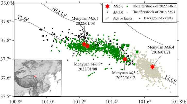
FIGURE 1. Spatial distribution of epicenters. The black dots represent background events before the Menyuan MS6.9 since 1970. The gray dot represents the 2016 MS6.4 Menyuan earthquake sequence, and the green dots represent the 2022 MS6.9 Menyuan earthquake sequence. LLLF stands for Lenglongling fault, NTLSF is the north Lenglongling fault, and TLSF is the Tuolaishan fault.
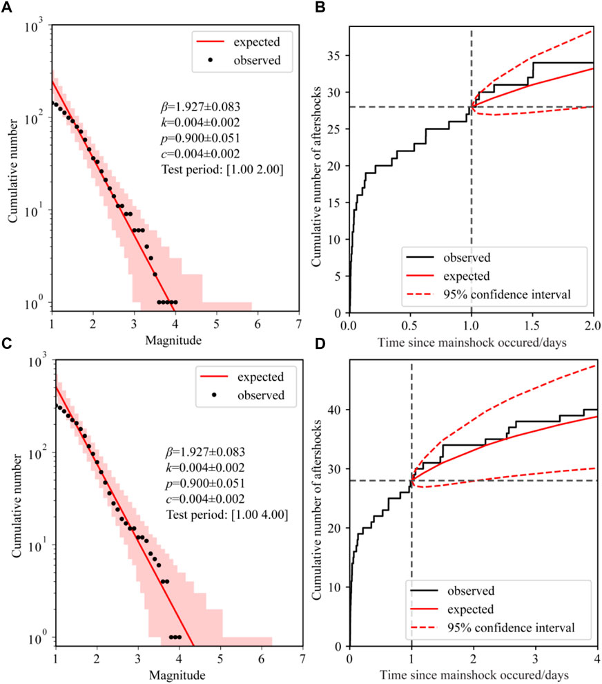
FIGURE 2. Future 1-day and 3-day aftershock forecasting for the Menyuan MS6.9 earthquake sequence using the Omi-R-J model. (A,B) Time period of 1.00–2.00 days and (C,D) time period of 1.00–4.00 days after the main shock. (A,C) Comparison of magnitude–cumulative frequency between forecasting (red lines) and actual observed aftershocks (black dots) and their 95% confidence intervals (pink areas). (B,D) Comparison of magnitude–cumulative frequency between forecasting (red curves) and actual observed aftershocks (black curves) of M>2.95 and their 95% confidence intervals (red dashed lines), and the forecasting starting and ending times (black vertical dashed lines) are delineated.
The N-test was intended to measure how well the total number of forecasted earthquakes matched the number of events observed. We used a one-sided test with an effective significance value, αeff, which is half of the intended significance value, α. In other words, we intended to maintain an error rate of α= 5% and to compare both δ1 and δ2 with a critical value of αeff = 0.025. If δ1 is less than αeff, the forecast rate is too low (under-prediction) and if δ2 is less than αeff, the forecast rate is too high (over-prediction). To quantitatively investigate the accuracy of the forecasted occurrence rates of strong aftershocks for different target magnitudes, MT = [3.0, 3.5, 4.0] of the MS6.9 Menyuan earthquake sequence, the N-test method was used to evaluate the performance results (Figure 3). The gray vertical line denotes the connection between the δ1 score and the δ2 score. Black diamonds and blue squares represent the results of δ1<0.025 and δ2<0.025, respectively. There is no blue square (δ2 <0.025) in Figure 3, which indicates that there was no over-prediction in the forecasting period. The Omi-R-J method shows good forecasting ability for early strong aftershocks, and the blank space indicates that the actual number of earthquakes was zero. Ignoring the influence of ‘no earthquakes’, there was no over-prediction forecasting. The Omi-R-J model had 9, 8, and 7 forecasting failures before and after the strong aftershocks of MS5.2 with respect to MT = [3.0, 3.5, 4.0]; thus, for complex earthquake sequences, the Omi-R-J model with good fitting performance has some limitations. Further analysis of the period of forecasting failure shows that before and after the MS5.2 strong aftershock of January 12, there was obvious under-prediction forecasting, which coincides with the main period of forecasting failure.
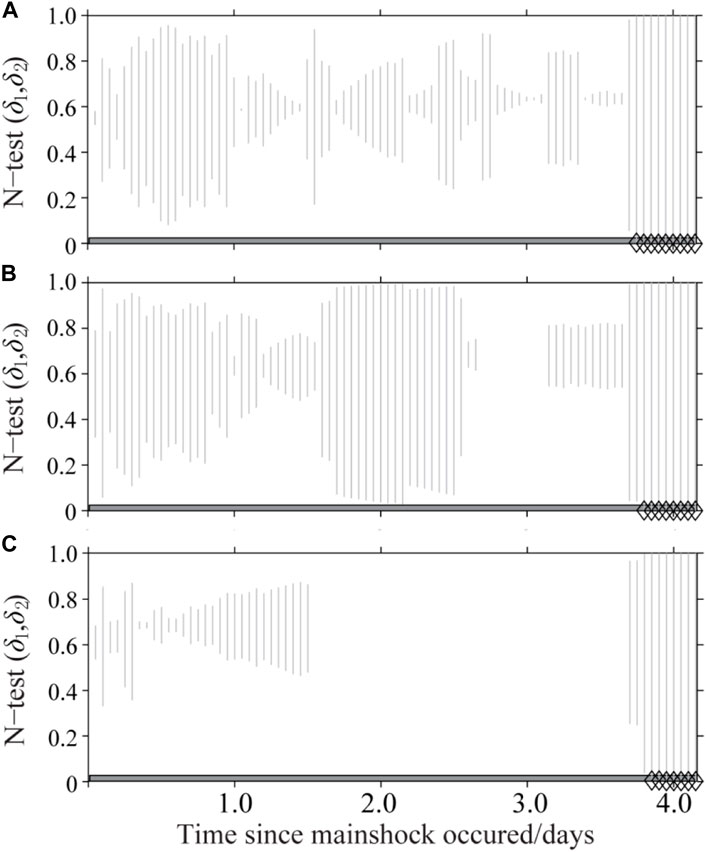
FIGURE 3. N-test results for future 1-day aftershock forecasting of the Menyuan MS6.9 earthquake sequence. (A–C) Forecasting performance evaluation of the Omi-R-J model for the three target magnitudes, 3.0, 3.5, 4.0, respectively. The vertical gray dashed lines connect the δ1 and δ2 values, while the black diamonds and blue squares show the results with δ1<0.025 and δ2<0.025, respectively. The blank area indicates that no event of corresponding magnitudes have occurred in the forecasting period.
Data-driven technology provides a new solution to the problem of subjectivity of model selection in the calculation of seismicity parameters. In this paper, we utilized the time-sequence b-value data-driven (TbDD) method proposed by Jiang et al. (2021a) to analyze the MS6.9 Menyuan earthquake sequence. The TbDD method consists of three major steps:
1) Selection of the magnitude–frequency distribution function. TbDD adopts the OK1993 model of a continuous distribution function given by Ogata and Katsura (1993) in a magnitude–frequency distribution relationship, which makes it superior by simultaneously determining the minimum magnitude of completeness and obtaining b-values.
2) Random partitioning in the time axis. In the model construction, it is necessary to randomly partition the given research time period [t0, t1] between the start time, t0, and the end time, t1.① A random number generator was used to generate random time nodes, T = {T1, T2, … , Tk}, where k is the number of time nodes. Correspondingly, the time period [t0, t1] was divided into time segments S = {S1, S2, … , Sk+1}, which constitute a model. ② We repeated step ① w times to obtain the w group partitioning schemes {Pi, i = 1, 2, … , w} on the time axis, that is, w models. ③ We repeated the aforementioned partitioning steps ① and ② with increasing k from 1 to n, where n is the maximum number of time nodes. For the time segments S = {S1, S2, … , Sk+1} of each model (or each partitioning scheme), the parameters of the OK1993 model [β, μ, σ] can be calculated using the events included in each time segment, and the total number of calculations was w×(n+1) times.
For any moment ti in the time interval (t0, t1), the b-value is derived from the events both before and after ti. For the moment t0, the b-value is calculated by using only the events after t0, and for the moment t1, the b-value is obtained by using only the events before t1. Therefore, only at the moment of t1, the TbDD method has the characteristic of forward-forecasting. As time continues to move forward, the b-value at the original t1 will be changed and updated.
3) Selection of the optimal models and calculation of ensemble median b-values. In order to select the optimal models most likely to reflect the final calculation results among a large number of models, the TbDD method adopted Bayesian information criteria (BIC) (Schwarz, 1978):
where
We implemented TbDD to calculate the b-values of the MS6.9 Menyuan earthquake sequence, attempting to use different maximum time segments (n+1) and different partitioning times (w). The models with the 5% lowest BIC values were taken as the optimal models, and the ensemble median values of the b-values were calculated as the final result. The BIC value distribution and the b-values of time sequences with the number of time segments n + 1 = {2,3,...11} and w = 100 are shown in Figures 4A,B, separately. For the partitioning with n + 1 = {2,3,...21} and w = 300, the results are shown in Figures 4C,D and for the partitioning with n + 1 = {2,3,...21} and w = 1000, the results are shown in Figures 4E,F. From the aforementioned calculation results, it can be seen that the b-values obtained under different combinations of maximum time segments (n + 1) and various partitioning times w are relatively close, which confirms the stability of the TbDD method. It is worth noting that, from 1.3 days before the January 12 MS5.2 strong aftershock, the b-value dropped significantly, from b = 0.93 to b = 0.63, with a drop as high as △b = 0.30, which is the only time that the b-value of aftershocks dropped significantly over the study period. This phenomenon makes it possible to give an alarm before this strong aftershock.
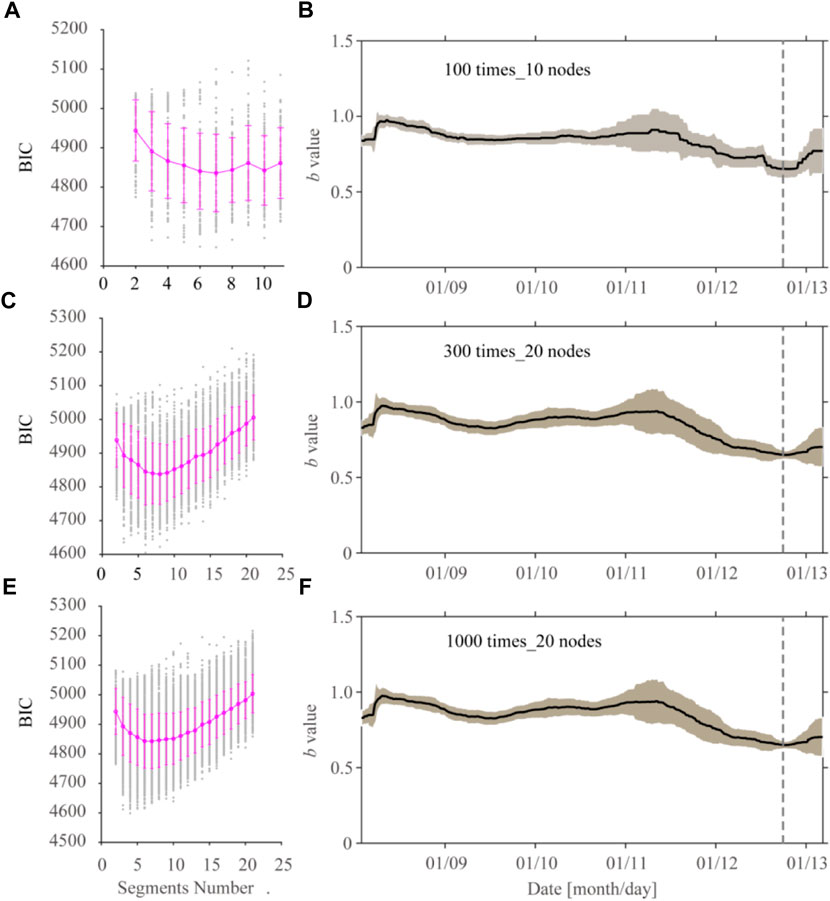
FIGURE 4. TbDD method calculation results for the 8 January 2022 Menyuan MS6.9 earthquake sequence. (A,C,E) BIC value distribution under different partition periods. The gray dots denote the calculation results of BIC values, and the pink dots and vertical lines denote the corresponding means and standard deviations of the BIC values, respectively. (B,D,F) Time-sequence changes of b-values calculated by TbDD. The black curves indicate the ensemble medians of b-values, the gray areas indicate the MAD of corresponding b-values, and the gray vertical dotted lines show the time of occurrence of strong aftershocks of the Menyuan MS5.2 aftershock on 12 January 2022.
To obtain a general threshold standard for the b-value changes of time series of strong aftershock risk alerts, which we used as a reference to conduct the strong aftershock forecasting of the MS6.9 Menyuan earthquake sequence, we studied the b-value changes of time series before strong aftershocks of M≥5.0 based on 86 intraplate earthquake sequences in the China continent whose main shock had a magnitude of MS≥6.0, as screened by Bi et al. (2022).We used the National Unified Official Catalogue produced by the China Earthquake Networks Center (CENC). Since 1 January 1970, the catalog has provided earthquake locations, occurrence times, and local magnitudes, ML, obtained using the same formula (Mignan et al., 2013). Thus the homogeneity of the reported magnitude was ensured for the whole period. Since the National Unified Official Catalogue starts from 1970, earthquakes were selected from the period between 1970/01/01 and the time immediately before each of 86 main shocks, as well as spatial restrictions on the distribution of aftershocks. Then we used the Gardner–Knopoff method (Gardner and Knopoff, 1974) to decluster catalogs to obtain the background seismicity of the corresponding earthquake sequence. Because of the absence of a large number of aftershock events in the early post-earthquake period, which seriously affected the stability of model parameters, only the events from 0.50 days after the main shock to the occurrence of the strongest aftershock were used to ensure the stability and quality of parameter fitting. Additionally, both the number of background events and aftershocks of the selected earthquake sequence amounted to no fewer than 30 results in a total of 34 earthquake sequences. The parameters of 34 main shocks are shown in Table 1, and the spatial distribution of the epicenters of the main shocks is mapped in Figure 5A.
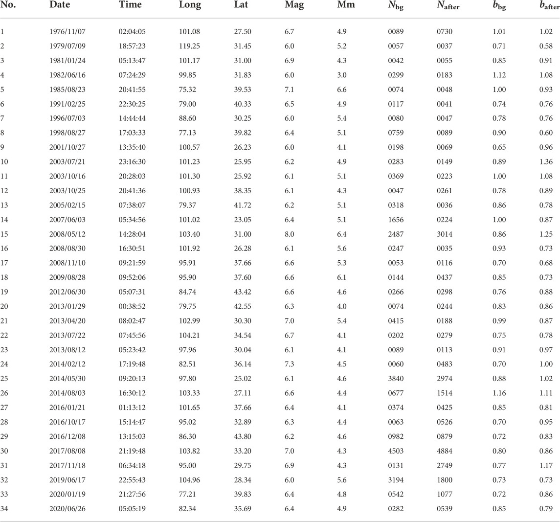
TABLE 1. Sequence parameters of intraplate earthquakes built for the SATLS in the China continent.
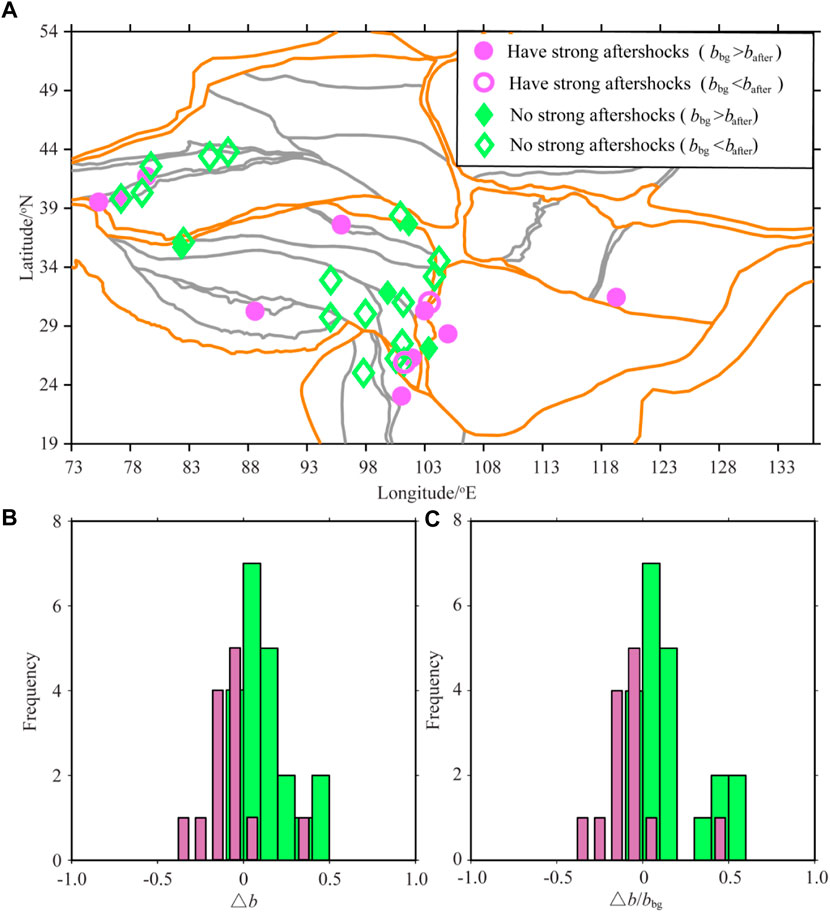
FIGURE 5. Distribution characteristics of 34 MS≥6.0 earthquake sequences in the China continent. (A) Distribution of the epicenters of the main shocks. They are classified according to the presence or absence of strong aftershocks of M≥5.0 and the relative size relationship between b-values of background events (bbg) and that of aftershocks (bafter), and indicated by different colors. The brown represents the boundary line of the primary plate, and the gray represents the boundary line of the secondary plate. (B) Statistical distribution of differences between background events bbg and aftershock bafter, △b. (C) Statistical relationship of △b/bbg. In (B,C), light red represents the earthquake sequences having strong aftershocks of M≥5.0, and light green represents the earthquake sequences having no strong aftershocks of M≥5.0.
The parameters of 34 earthquake sequences were fitted using the OK1993 model, and the b-values of both background events (bbg) and aftershocks (bafter) are shown in Table 1. Statistical analyses indicated 13 earthquake sequences with M≥5.0 aftershocks. The average was bbg = 0.87 ± 0.11 and bafter = 0.81 ± 0.19, and bbg>bafter accounted for 84.62% (11/13) and bbg<bafter accounted for 15.38% (2/13); there were 21 earthquake sequences without strong M≥5.0 aftershocks in the fitting period, with average bbg = 0.83 ± 0.13 and bafter = 0.95 ± 0.15, of which bbg>bafter accounted for 19.05% (4/21) and bbg<bafter accounted for 80.95% (17/21). The statistical distribution of the differences in b-values between the background events bbg and the aftershocks bafter, (△b = bafter - bbg), and the ratio △b/bbg are given in Figures 5B,C. The results show that the mean △b value and the median △b value of the sequences having strong aftershocks of M≥5.0 were −0.13 and −0.16, separately, and that the mean and the median of △b/bbg were −0.06 and −0.08, separately. However, the △b of the sequences without strong aftershocks of M≥5.0 had a mean value of 0.27 and a median value of 0.15, and the mean value of △b/bbg was 0.16 and the median value was 0.08.
The aforementioned analysis shows that bafter<bbg for the sequences with M≥5.0 aftershocks and bafter>bbg for the sequences without M≥5.0 aftershocks are statistically significant. If we conduct the risk assessment of M≥5.0 aftershocks according to the aforementioned relationship, it can be seen that when △b>0, two earthquake sequences have M≥5.0 aftershocks, and 17 earthquake sequences have no aftershocks with M≥5.0; when △b<0, eleven earthquake sequences have M≥5.0 aftershocks, and four earthquake sequences have no aftershocks with M≥5.0. Furthermore, when △b>0.1, only one earthquake event had aftershocks of M≥5.0, while when △b<-0.1, all earthquake sequences had aftershocks of M≥5.0. The statistical results are illustrated in Figure 6A. This shows that the possibility of strong aftershocks with M≥5.0 can be reliably determined by defining △b=±0.1. Moreover, from Figure 6A, when △b<0, especially △b<-0.1, the magnitude difference between a main shock and its largest aftershock mainly ranged from 0 to 1.5. While, when △b>0, the magnitude difference ranged from 1.5 to 3.0.
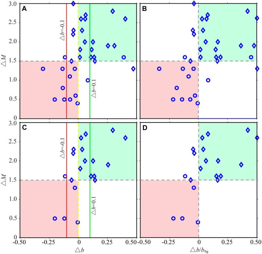
FIGURE 6. Relationship between magnitude difference and sequence parameters. (A) Relationship between △M and △b (△b = bafter - bbg) (1970.01.01–2020.07.30); (B) relationship between △M and △b/bbg (1970.01.01–2020.07.30); (C) relationship between △M and △b of the sequences after 12 May 2008; (D) relationship between △M and △b/bbg of the sequences after 12 May 2008. The circle represents the earthquake sequence having strong aftershocks with M≥5.0, and the diamond represents the earthquake sequence having no strong aftershocks with M≥5.0 in the fitting period. The red, yellow, and green lines indicate △b = 0.1, △b = 0 and △b = -0.1, respectively. The green area represents △M>1.5 and △b>0, while the red area represents △M<1.5 and △b<0.
The earthquake monitoring capability of the China Earthquake Networks Center was significantly improved after the 2008 MS8.0 Wenchuan earthquake (Huang et al., 2017). To eliminate the influence of the change in earthquake monitoring capability, we excluded the earthquake sequences before the 2008 MS8.0 Wenchuan earthquake and investigated the relationship between △b and the occurrence of strong aftershocks of M≥5.0. The results demonstrate that all earthquake sequences have no strong aftershocks with M≥5.0 when △b>0.1, while when △b<-0.1, all earthquake sequences have strong aftershocks with M≥5.0 (Figure 6C). In addition, we also used △b/bbg for similar analyses, and found the same risk classification effectiveness using △b/bbg = ±0.1 as using △b = ±0.1, as shown in Figures 6B,D.
Based on the aforementioned calculations, we defined △b = 0.1 as the green threshold with low risk of M≥5.0 strong aftershocks, that is, when △b≥0.1, the possibility of M≥5.0 strong aftershocks is low; △b = -0.1 is a high-risk red threshold for strong aftershocks with M≥5.0. When △b is lower than this threshold, that is △b≤-0.1, the possibility of strong aftershocks with M≥5.0 is high; △b = 0 represents a distinct yellow threshold. When -0.1<△b<0.1, we should pay attention to the occurrence of strong M≥5.0 aftershocks. By combination with the TbDD method based on data-driven technology to calculate bbg, bafter, and △b, a strong aftershock traffic light system (SATLS) was constructed to accurately determine the risk of strong M≥5.0 aftershocks in real time, which makes it feasible to make targeted disaster mitigation decisions.
We performed SATLS classification of the occurrence of strong aftershocks with M≥5.0 for the 2022 MS6.9 Menyuan earthquake sequence followed by only two aftershocks of M≥5.0. The MS5.1 aftershock occurred within just a few hours after the main shock, and the poor data availability before this event may result in large uncertainties in the b-values. Therefore, only the January 12 MS5.2 aftershock was discussed here. The data for calculation were obtained from the National Unified Official Catalogue, and the spatial range covered was the same as the distribution of aftershocks. The events from 1970 to the time before the main shock were taken as background events, and those between the main shock and the MS5.2 aftershock were taken as aftershock sequences.
The results showed that bbg = 0.83 and bafter = 0.81, and the corresponding fitting curves of the OK1993 model are shown in Figures 7A,B. Because bafter<bbg, it can be determined that the yellow threshold of SATLS has been reached. The b-values of the time series were calculated by TbDD as shown in Figure 7C. Before the MS5.2 aftershock, the b-value had dropped to about 0.79, that is, △b≈-0.04, according to which a yellow alert for the possibility of a strong aftershock with M≥5 would be declared.
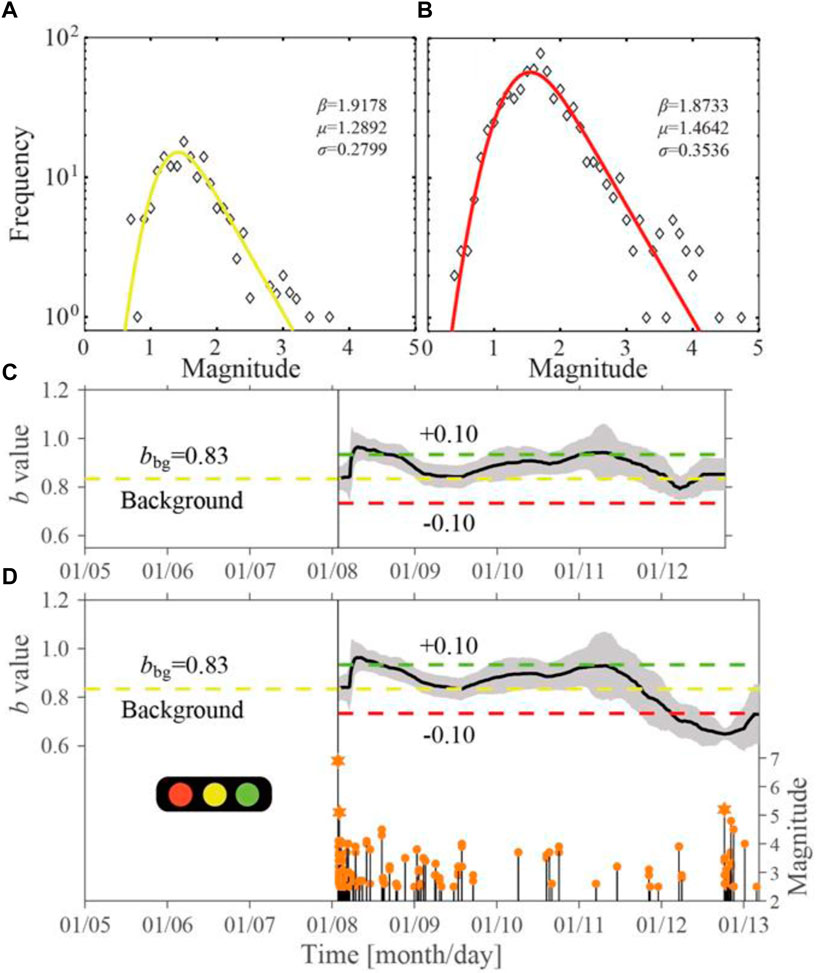
FIGURE 7. Characteristics of the b-value evolution for the 8 January 2022 Menyuan MS6.9 earthquake sequence and SATLS settings. (A,B) Magnitude–frequency distribution (FMD) and the fitting results of the OK1993 model. They correspond to the background earthquake sequence (1970.01.01∼2022.01.08) and aftershock sequence (2022.01.08∼2022.01.12), respectively. The diamonds denote the FMD of the events. The solid curve indicates the fitting results of the OK1993 model, and the actual parameters are marked in each subgraph in the order of β, μ, and σ. (C) b-value of time series obtained using the events immediately before the strong aftershock (2022.01.08∼2022.01.12). (D) b-value of time series calculated using the events between the main shock and the time after the strong aftershock (2022.01.08∼2022.01.13). The yellow dotted line indicates background value bbg (yellow threshold), the red dotted line denotes the red threshold (0.1 lower than the background value), the green dotted line represents the green threshold (0.1 higher than the background value), and the magnitude–time distribution (M-t) of the earthquake sequence is displayed.
We further investigated the b-values of the time-series between the main shock and the time after the MS5.2 aftershock as shown in Figure 7D. The results indicated that before the MS5.2 strong aftershock, the b-value decreased to about 0.63, △b≈-0.2, the magnitude of which is larger than that of △b≈-0.04, as obtained using events between the main shock and the MS5.2 aftershock. After the MS5.2 strong aftershock, the stress around the focal area changed and the b-value continued to decrease. Yang et al. (2022) obtained the background b-value of 0.84 using the maximum-likelihood method and the whole aftershock b-value of 0.67 using the least-squares method for the Menyuan earthquake, and our results were similar to theirs. The h-value is a constant in the revised Omori’s law which describes the number of aftershocks after the main shock. It can be used to determine whether there might be future events with larger magnitudes during an ongoing sequence (Liu et al., 1979). If h≫1, it indicates that the largest magnitude earthquake already occurred as the main shock. If h≪1, then it was considered a foreshock sequence. The 2022 Menyuan sequence showed that the overall h-value was significantly larger than 1. (Yang et al., 2022).
The SATLS proposed in this paper is, in a more general sense, an extension of the FTLS which determined whether an event was a main shock or a foreshock to an even stronger event yet to come. However, there are several limitations to the SATLS. First, the threshold settings of the SATLS are only based on a limited number of earthquake cases, and it is only suitable for the intraplate earthquake sequences of the M≥6.0 main shock in the China continent followed by M≥5.0 aftershocks. Moreover, there is a lack of systematic and comprehensive understanding of the relative relationship between the values of bafter and bbg in different tectonic regions, which limits the general applicability of the SATLS. In addition, some researchers argue that the spatial distribution of b-values is highly variable. For example, the ductile shear zone has a higher b-value than the brittle-ductile shear zone (Villiger et al., 2020). Also, it is easy for a high b-value to be produced in rocks with low Young’s modulus (Zorn et al., 2019) or high organic content, which causes difficulties in the application of SATLS for earthquake sequences with large-scale spatial distribution in aftershock zones, and it may be necessary to develop a set of two-dimensional time-space △b risk classification thresholds. There are also some shortfalls in this research. Thirty-four events may not be enough to derive exact thresholds. With respect to the whole b-value calculated by the OK1993 model, the uncertainty and the confidence interval of the whole b-value has not been resolved, which needs to be addressed in subsequent research.
During revision of this paper, there occurred in China on 5 September 2022, the MS6.8 Luding earthquake with an MS5.0 aftershock, which provided a new opportunity to verify the effectiveness of the SATLS. Therefore, along with the Menyuan earthquake, we also applied SATLS to the MS6.8 2022 Luding earthquake sequence. We obtained bbg = 0.9672 from the OK1993 model and b-values of time series by TbDD. The results showed that three days before the MS5.0 earthquake, the b-value started to decrease. As of 13:17 on October 23 when the MS5.0 aftershock occurred, the b-value had decreased to about 0.86, for a △b ≈ -0.1, which suggests that a red alert could have been declared for a strong aftershock of M≥5.0. To some extent, this event demonstrates the effectiveness of SATLS.
Although the N-test results showed that the Omi-R-J model failed in forecasting the strong MS5.2 aftershock, the failure reason could not rule out the possibility that the Omi-R-J method is based on the Omori–Utsu formula with a relatively simple aftershock attenuation law, and it only demonstrates obvious forecasting effectiveness for aftershock sequences with underdeveloped secondary aftershocks. For more complex earthquake sequences, the analysis may need to be combined with the ETAS model. In fact, CSEP also focuses on the predictability of some huge earthquake cases (Schorlemmer et al., 2018). For example, after the 2011 M9.0 earthquake in East Japan, Nanjo et al. (2012) and Ogata et al. (2013) systematically tested the forecasting effectiveness of various versions of the ETAS model and confirmed that it showed good forecasting performance on complex aftershock sequences. In the future, a combination of the semi-quantitative and semi-qualitative SATLS and the quantitative statistical probability forecasting models is still a realistic and feasible choice.
It is difficult to accurately forecast a disaster-causing aftershock using only traditional statistical forecasting models. We first used the TbDD method based on data-driven technology to obtain reliable b-values of time series. Second, based on the empirical relationship, △b = bafter - bbg, from 34 M≥6.0 intraplate earthquake sequences in the China continent and their strongest aftershocks of M≥5.0, a strong aftershock traffic light system (SATLS) was constructed. Taking the 8 January 2022 MS6.9 Menyuan earthquake in Qinghai Province as an example, a yellow alert attempt was made by using SATLS for the MS5.2 strong aftershocks that occurred several days after the main shock. The main results are summarized as follows:
1) The Omi-R-J model for aftershock probability forecasting was employed to conduct 83 consecutive sliding forecasts of strong aftershocks of the MS6.9 Menyuan earthquake sequence, and the forecasting performance was assessed by the N-test method. The results showed that the earthquake occurrence rates forecast by the Omi-R-J model before the largest aftershock (MS5.2) were too low; however, the model can accurately forecast aftershock rates for each magnitude interval in most time-periods, which makes it difficult to accurately forecast this strong aftershock.
2) The data from our research on the 34 M≥6.0 intraplate earthquake sequences in the China continent showed that △b = bafter - bbg =±0.1 can act as a discriminator to determine whether strong aftershocks of magnitude 5.0 or higher will occur. If the difference (△b = bafter - bbg) exceeded +0.1 (△b = 0.1) or was -0.1 (△b = -0.1), we assigned a traffic light color of green or red, respectively, otherwise yellow. We can further infer the possible magnitude of an aftershock based on the relationship between △M and △b.
3) The b-value calculation of the MS6.9 Menyuan earthquake sequence using TbDD showed that, for different time partitioning schemes, random partitioning times, and other technical rules, the perturbation of determined time series b-values was negligible. The b-value obtained using the events between the main shock and the MS5.2 event decreased 0.04 (△b ≈ -0.04) from 1.3 days before the MS5.2 strong aftershock, while the b-value calculated using the events between the main shock and the time after the MS5.2 earthquake decreased 0.2 and gradually recovered after this strong aftershock. From the time-series of b-values of the 2022 MS6.9 Menyuan earthquake sequence, before the MS5.2 event, only a yellow alert could be declared, which shows a gap from the expected determined red alert. One reason may be that it is questionable if the seismicity before an M≥5.0 strong aftershock could reveal the stress status of that moment. The fact that a strong aftershock of M≥5.0 abruptly changes the stress status in the focal area may be another factor. To improve the accuracy of forecast making, a deeper understanding of the true b-value and the detailed description of the stress evolution state in the source area is needed.(Gutenberg and Richter, 1944; Nandan et al., 2017; Si and Jiang, 2019; Jiang et al., 2021).
The earthquake catalog used in this paper was provided by the China Earthquake Networks Center. The Multi-Parametric Toolbox 3.0 (https://www.mpt3.org/Main/HomePage, last accessed February 2022) is used for the analysis of parametric optimization.
The original contributions presented in the study are included in the article/Supplementary Material, and further inquiries can be directed to the corresponding author.
JB, FY, and CJ contributed to conceptualization. JB prepared the manuscript with contributions from all authors. JB, FY, and CJ wrote software for data processing. XY, YM, and CS contributed to the revised manuscript version.
This study was supported by the Joint Funds of the National Natural Science Foundation of China and the Foundation of Earthquake Science (U1839207), the Special Fund of the Institute of Geophysics, China Earthquake Administration (DQJB22Z01) and the 2022 Earthquake Regime Tracking Work of the CEA (2022010116).
The authors thank Yan Zhang and Hongyu Zhai of the Institute of Geophysics, China Earthquake Administration, for their constructive suggestions on this paper. We also thank the editor and two anonymous reviewers for their very helpful comments and suggestions. This study used the National Unified Official Catalogue provided by the China Earthquake Networks Center.
The authors declare that the research was conducted in the absence of any commercial or financial relationships that could be construed as a potential conflict of interest.
All claims expressed in this article are solely those of the authors and do not necessarily represent those of their affiliated organizations, or those of the publisher, the editors, and the reviewers. Any product that may be evaluated in this article, or claim that may be made by its manufacturer, is not guaranteed or endorsed by the publisher.
Bi, J. M., and Jiang, C. S. (2020). Comparison of early aftershock forecasting for the 2008 Wenchuan MS8.0 earthquake. Pure Appl. Geophys. 177, 9–25. doi:10.1007/s00024-019-02192-6
Bi, J. M., Jiang, C. S., Lai, G. J., and Song, C. (2022). Effectiveness evaluation and constraints of early aftershock probability forecasting for strong earthquakes in continental China. Chin. J. Geophys. (in Chinese) 65 (7), 2532–2545. doi:10.6038/cjg2022P0411
Bi, J. M., Jiang, C. S., and Ma, Y. (2020). The study on early sequence parameters and probability forecasting of strong aftershocks of Changning MS6.0 earthquake on June 17, 2019, Sichuan Province. Earthquake (in Chinese) 40 (2), 140–154. doi:10.12196/j.issn.1000-3274.2020.02.011
Chan, L. S., and Chandler, A. M. (2001). Spatial bias in b-value of the frequency–magnitude relation for the Hong Kong region. Journal of Asian Earth Sciences 20 (1), 73–81. doi:10.1016/s1367-9120(01)00025-6
Gardner, J. K., and Knopoff, L. (1974). Is the sequence of earthquakes in Southern California with aftershocks removed, Poissonian? Bulletin of the Seismological Society of America 64, 1363–1367. doi:10.1785/bssa0640051363
Grimm, C., Käser, M., Hainzl, S., Pagani, M., and Kuchenhoff, H. (2021). Improving earthquake doublet frequency predictions by modified spatial trigger kernels in the Epidemic-Type Aftershock Sequence (ETAS) Model. Bull. Seismol. Soc. Am. 112 (1), 474–493. doi:10.1785/0120210097
Gulia, L., Rinaldi, A. P., Tormann, T., Vannucci, G., Enescu, B., and Wiemer, S. (2018). The effect of a mainshock on the size distribution of the aftershocks. Geophys. Res. Lett. 45, 13277–13287. doi:10.1029/2018GL080619
Gulia, L., and Wiemer, S. (2019). Real-time discrimination of earthquake foreshocks and aftershocks. Nature 574 (7777), 193–199. doi:10.1038/s41586-019-1606-4
Gulia, L., Wiemer, S., and Vannucci, G. (2020). Pseudoprospective evaluation of the foreshock traffic-light system in Ridgecrest and implications for aftershock hazard assessment. Seismological Research Letters 91 (5), 2828–2842. doi:10.1785/0220190307
Gutenberg, R., and Richter, C. F. (1944). Frequency of earthquakes in California. Bulletin of the Seismological Society of America 34, 185–188. doi:10.1785/bssa0340040185
Huang, F. Q., Li, M., Ma, Y. C., Han, Y., Tian, L., Yan, W., et al. (2017). Studies on earthquake precursors in China: A review for recent 50 years. Geodesy and Geodynamics 8 (1), 1–12. doi:10.1016/j.geog.2016.12.002
Iwata, T. (2013). Estimation of completeness magnitude considering daily variation in earthquake detection capability. Geophysical Journal International 194 (3), 1909–1919. doi:10.1093/gji/ggt208
Jiang, C., Qiu, Y., Jiang, C. S., Yin, X. X., Zhai, H. Y., Zhang, Y. B., et al. (2021a). A new method for calculating b-value of time sequence based on data-driven (TbDD): A case study of the 2021 yangbi MS6.4 earthquake sequence in yunnan. Chinese Journal of Geophysics (in Chinese) 64 (9), 3126–3134. doi:10.6038/cjg2021P0385
Jiang, C., Jiang, C. S., Yin, F. L., Zhang, Y. B., Bi, J. M., Long, F., et al. (2021b). Traffic light system (TLS) for risk control of earthquake induced by industrial activities: Problem and prospects. Progress in Geophysics (in Chinese) 36 (6), 2320–2328. doi:10.6038/pg2021EE0495
Jiang, C. S., Bi, J. M., Wang, F. C., et al. (2018). Application of the Omi-R-J method for forecast of early aftershocks to the 2017 Jiuzhaigou, Sichuan, MS7.0 earthquake. Chinese Journal of Geophysics (in Chinese) 61, 2099–2110. doi:10.6038/cjg2018M0113
Jiang, C. S., Han, L. B., Long, F., Lai, G., Yin, F., Bi, J., et al. (2021). Spatiotemporal heterogeneity of b values revealed by a data-driven approach for June 17, 2019 MS 6.0, Changning Sichuan, China earthquake sequence. Nat. Hazards Earth Syst. Sci. 21, 2233–2244. doi:10.5194/nhess-21-2233-2021
Kagan, Y. Y., and Jackson, D. D. (1995). New seismic gap hypothesis: Five years after. J. Geophys. Res. 100 (B3), 3943–3959. doi:10.1029/94jb03014
Lippiello, E., Giacco, F., Marzocchi, W., Godano, G., and Arcangelis, L. d. (2017). Statistical features of foreshocks in instrumental and ETAS catalogs. Pure Appl. Geophys. 174 (4), 1679–1697. doi:10.1007/s00024-017-1502-5
Liu, Z. R., Qian, Z. X., and Wang, W. Q. (1979). Decay in earthquake frequency, an indicator of foreshocks. Journal of Seismological Research (in Chinese) 2 (4), 1–9.
Lv, X. J., Gao, M. T., Gao, Z. W., and Mi, S. T. (2007). Comparison of the spatial distribution of ground motion between mainshocks and strong aftershocks. Acta Seismologica Sinica (in Chinese) 29 (3), 295–301. doi:10.1007/s11589-007-0312-8
Matsu'ura, R. S. (1986). Precursory quiescence and recovery of aftershock activities before some large aftershocks. Bulletin of the Earthquake Research Institute 61, 1–65.
Mignan, A., Jiang, C. S., Zechar, J. D., Wiemer, S., Wu, Z., and Huang, Z. (2013). Completeness of the mainland China earthquake catalog and implications for the setup of the China earthquake forecast testing center. Bulletin of the Seismological Society of America 103 (2A), 845–859. doi:10.1785/0120120052
Mignan, A., and Woessner, J. (2012). Estimating the magnitude of completeness for earthquake catalogs. CORSSA Community Online Resource for Statistical Seismicity Analysis. doi:10.5078/corssa-00180805
Nandan, S., Ouillon, G., Wiemer, S., and Sornette, D. (2017). Objective estimation of spatially variable parameters of epidemic type aftershock sequence model: Application to California. J. Geophys. Res. Solid Earth 122 (7), 5118–5143. doi:10.1002/2016JB013266
Nanjo, K. Z., Izutsu, J., Orihara, Y., and Kamogawa, M. (2022). Changes in seismicity pattern due to the 2016 Kumamoto earthquake sequence and implications for improving the foreshock traffic-light system. Tectonophysics 822, 229175. doi:10.1016/j.tecto.2021.229175
Nanjo, K. Z., Tsuruoka, H., Yokoi, S., Ogata, Y., Falcone, G., Hirata, N., et al. (2012). Predictability study on the aftershock sequence following the 2011 Tohoku-Oki, Japan, earthquake: First results. Geophys. J. Int. 191, 653–658. doi:10.1111/j.1365-246X.2012.05626.x
Ogata, Y., and Katsura, K. (1993). Analysis of temporal and spatial heterogeneity of magnitude frequency distribution inferred from earthquake catalogues. Geophys. J. Int. 113 (3), 727–738. doi:10.1111/j.1365-246x.1993.tb04663.x
Ogata, Y., Katsura, K., Falcone, G., Nanjo, K., and Zhuang, J. (2013). Comprehensive and topical evaluations of earthquake forecasts in terms of number, time, space, and magnitude. Bulletin of the Seismological Society of America 103 (3), 1692–1708. doi:10.1785/0120120063
Ogata, Y. (2001). Increased probability of large earthquakes near aftershock regions with relative quiescence. J. Geophys. Res. 106, 8729–8744. doi:10.1029/2000jb900400
Ogata, Y. (2006). Monitoring of anomaly in the aftershock sequence of the 2005 earthquake of M7.0 off coast of the Western Fukuoka, Japan, by the ETAS model. Geophys. Res. Lett. 33, L01303. doi:10.1029/2005GL024405
Ogata, Y. (1989). Statistical model for standard seismicity and detection of anomalies by residual analysis. Tectonophysics 169 (1/2/3), 159–174. doi:10.1016/0040-1951(89)90191-1
Omi, T., Ogata, Y., Hirata, Y., and Aihara, K. (2013). Forecasting large aftershocks within one day after the main shock. Sci. Rep. 3, 2218. doi:10.1038/srep02218
Omi, T., Ogata, Y., Hirata, Y., and Aihara, K. (2015). Intermediate-term forecasting of aftershocks from an early aftershock sequence: Bayesian and ensemble forecasting approaches. J. Geophys. Res. Solid Earth 120 (4), 2561–2578. doi:10.1002/2014JB011456
Omi, T., Ogata, Y., Shiomi, K., Enescu, B., Sawazaki, K., and Aihara, K. (2016). Automatic aftershock forecasting: A test using real-time seismicity data in Japan. Bulletin of the Seismological Society of America 106 (6), 2450–2458. doi:10.1785/0120160100
Omori, F. (1894) Tokyo, Japan. Imperial University of Tokyo, 111–200.On aftershocks of earthquakes, Doctoral dissertation.
Reasenberg, P. A., and Jones, L. M. (1989). Earthquake hazard after a mainshock in California. Science 243, 1173–1176. doi:10.1126/science.243.4895.1173
Scholz, C. H. (2015). On the stress dependence of the earthquake b-value. Geophys. Res. Lett. 42 (5), 1399–1402. doi:10.1002/2014GL062863
Scholz, C. H. (1968). The frequency-magnitude relation of microfracturing in rock and its relation to earthquakes. Bulletin of the Seismological Society of America 58 (1), 399–415. doi:10.1785/bssa0580010399
Schorlemmer, D., Gerstenberger, M. C., Wiemer, S., Jackson, D. D., and Rhoades, D. A. (2007). Earthquake likelihood model testing. Seismological Research Letters 78, 17–29. doi:10.1785/gssrl.78.1.17
Schorlemmer, D., Werner, M. J., Marzocchi, W., Jordan, T. H., Ogata, Y., Jackson, D. D., et al. (2018). The collaboratory for the study of earthquake predictability: Achievements and priorities. Seismological Research Letters 89 (4), 1305–1313. doi:10.1785/0220180053
Schwarz, G. (1978). Estimating the dimension of a model. Ann. Statist. 6 (2), 461–464. doi:10.1214/aos/1176344136
Shcherbakov, R. (2021). Statistics and forecasting of aftershocks during the 2019 Ridgecrest, California, earthquake sequence. J. Geophys. Res. Solid Earth 126, e2020JB020887. doi:10.1029/2020JB020887
Si, Z. Y., and Jiang, C. S. (2019). Research on parameter calculation for the Ogata-Katsura 1993 model in terms of the frequency-magnitude distribution based on a data-driven approach. Seismological Research Letters 90 (3), 1318–1329. doi:10.1785/0220180372
Trevlopoulos, K., Guéguen, P., Helmstetter, A., and Cotton, F. (2020). Earthquake risk in reinforced concrete buildings during aftershock sequences based on period elongation and operational earthquake forecasting. Structural Safety 84, 101922. doi:10.1016/j.strusafe.2020.101922
Utsu, T. (1961). A statistical study of on the occurrence of aftershocks. Geophysical Magazine 30, 521–605.
Villiger, L., Gischig, V. S., Doetsch, J., Krietsch, H., Dutler, N. O., Jalali, M., et al. (2020). Influence of reservoir geology on seismic response during decameter-scale hydraulic stimulations in crystalline rock. Solid Earth 11 (2), 627–655. doi:10.5194/se-11-627-2020
Woessner, J., Hainzl, S., Marzocchi, W., Werner, M. J., Lombardi, A. M., Catalli, F., et al. (2011). A retrospective comparative forecast test on the 1992 Landers sequence. J. Geophys. Res. 116, B05305. doi:10.1029/2010JB007846
Yang, H. F., Wang, D., Guo, R. M., Xie, M., Zang, Y., Wang, Y., et al. (2022). Rapid report of the 8 january 2022 menyuan Ms6.9 earthquake, Qinghai, China. Earthquake Research Advances 2 (1), 100113–100114. doi:10.1016/j.eqrea.2022.100113
Zechar, J. D. (2010). “Evaluating earthquake predictions and earthquake forecasts: A guide for students and new researchers, Community online resource for statistical seismicity analysis 126. doi:10.5078/corssa-77337879
Zhang, C. J., Hou, Y. Y., Hu, B., Xu, H. H., and Wang, D. B. (2011). Analysis on the seismic activities and hazards of M7.1 earthquake, 2010 and M6.3 earthquake, 2011 in New Zealand. Recent Developments in World Seismology 1 (4), 44–51. doi:10.3969/j.issn.0235-4975.2011.04.010
Keywords: Ogata–Katsura 1993 model, Omi–Reasenberg–Jones model, time-sequence b-value data-driven (TbDD) method, aftershock forecasting, traffic light system
Citation: Bi J, Yin F, Jiang C, Yin X, Ma Y and Song C (2023) Strong aftershocks traffic light system: A case study of the 8 January 2022 MS6.9 Menyuan earthquake, Qinghai Province, China. Front. Earth Sci. 10:994850. doi: 10.3389/feart.2022.994850
Received: 15 July 2022; Accepted: 15 November 2022;
Published: 16 January 2023.
Edited by:
Hongfeng Yang, The Chinese University of Hong Kong, ChinaReviewed by:
Andrea Llenos, U.S. Geological Survey, United StatesCopyright © 2023 Bi, Yin, Jiang, Yin, Ma and Song. This is an open-access article distributed under the terms of the Creative Commons Attribution License (CC BY). The use, distribution or reproduction in other forums is permitted, provided the original author(s) and the copyright owner(s) are credited and that the original publication in this journal is cited, in accordance with accepted academic practice. No use, distribution or reproduction is permitted which does not comply with these terms.
*Correspondence: Fengling Yin, eWluZmVuZ2xpbmdAY2VhLWlncC5hYy5jbg==; Changsheng Jiang, amlhbmdjc0BjZWEtaWdwLmFjLmNu
Disclaimer: All claims expressed in this article are solely those of the authors and do not necessarily represent those of their affiliated organizations, or those of the publisher, the editors and the reviewers. Any product that may be evaluated in this article or claim that may be made by its manufacturer is not guaranteed or endorsed by the publisher.
Research integrity at Frontiers
Learn more about the work of our research integrity team to safeguard the quality of each article we publish.