On the correlation between earthquake coda horizontal-to-vertical spectral ratios and amplification functions at the KiK-net network

The Japanese KiK-net network comprises about 700 stations spread across the whole territory of Japan. For most of the stations, V_P and V_S profiles were measured down to the bottom borehole station. Using the vast dataset of earthquake recordings from 1997 to 2020 at a subset of 428 seismic stations, we compute the horizontal-to-vertical spectral ratio of earthquake coda, the S-wave surface-to-borehole spectral ratio, and the equivalent outcropping S-wave amplification function. The de facto equivalence of the horizontal-to-vertical spectral ratio of earthquake coda and ambient vibration is assessed on a homologous Swiss dataset. Based on that, we applied the canonical correlation analysis between amplification information and the horizontal-to-vertical spectral ratio of earthquake coda across all KiK-net sites. The aim of the correlation is to test a strategy to predict local earthquake amplification basing the inference on site condition indicators and single-station ambient vibration recordings. Once the correlation between frequency-dependent amplification factors and amplitudes of horizontal-to-vertical coda spectral ratios is defined, we predict amplification at each site in the selected KiK-net dataset with a leave-one-out cross-validation approach. In particular, for each site, three rounds of predictions are performed, using as prediction target the surface-to-borehole spectral ratio, the equivalent of a standard spectral ratio referred to the local bedrock and to a common Japanese reference rock profile. From our analysis, the most effective prediction is obtained when standard spectral ratios referred to local bedrock and the horizontal-to-vertical spectral ratio of earthquake coda are used, whereas a strong mismatch is obtained when standard spectral ratios are referred to a common reference. We ascribe this effect to the fact that, differently from amplification functions referred to a common reference, horizontal-to-vertical spectral ratios are fully site-dependent and then their peak amplitude is influenced by the local velocity contrast between bedrock and overlying sediments. Therefore, to reduce this discrepancy, we add in the canonical correlation as a site proxy the inferred velocity of the bedrock, which improves the final prediction.

Introduction

Several studies have been conducted using the KiK-net recording dataset due to the availability of several thousands of joint surface/downhole strong-motion recordings (Okada et al., 2004; Aoi et al., 2011). In addition to the abundance of data, another main advantage of this network is that all sites are characterized in terms of velocity profiles (V_S, V_P). The KiK-net dataset is, therefore, ideal for studies focusing on site response (Régnier et al., 2018; Kawase et al., 2019; Bergamo et al., 2021). Some authors have defined strategies to derive from KiK-net surface-to-borehole spectral ratios the equivalent of empirical amplification functions referred to outcropping bedrock (Kokusho and Sato, 2008; Cadet et al., 2012a; Poggi et al., 2017; Tao and Rathje, 2020). Amplification values at the KiK-net stations have been compared and/or correlated with indirect proxies (Derras et al., 2017; Bergamo et al., 2021; Di Giulio et al., 2021) or with shear wave velocity (V_S) profile information (Cadet et al., 2012b; Poggi et al., 2019; Zhu et al., 2020; Bergamo et al., 2021). One of the aims of these correlations is to devise strategies to extrapolate amplification information at sites where the latter is unknown, basing the prediction on site proxies. Moreover, the KiK-net velocity profiles can be used to derive SH-transfer functions (Kaklamanos et al., 2015; Pilz and Cotton, 2019) or to apply methods such as those based on the quarter-wavelength representation (Joyner et al., 1981; Boore, 2003). Furthermore, time-averaged shear wave velocity from the surface to a depth of 30 m (V_S30) can be easily obtained to classify the seismic stations according to worldwide seismic codes (CEN, 2004; BSSC, 2009).

In light of these applications aiming at retrieving amplification information from site proxies, Cultrera et al. (2014) and Panzera et al. (2021) linked through canonical correlation (CC) the horizontal-to-vertical spectral ratio of noise (HVSRn; Nakamura, 1989) with empirical site amplification functions. Cultrera et al. (2014) used a worldwide dataset of HVSRn and site-to-reference spectral ratios (SSR; Borcherdt, 1970), whereas Panzera et al. (2021) used a Swiss dataset of co-located HVSRn and empirical spectral modeling amplification functions (ESM; Castro et al., 1990; Field and Jacob, 1995; Oth et al., 2011; Edwards et al., 2013). The results highlight the ability of the method to provide an estimate of the local earthquake amplification over chosen frequency bins for sites where single-station ambient vibration recordings are available. In this study, we apply CC to a set of KiK-net seismic stations for which we computed the horizontal-to-vertical spectral ratio of earthquake coda (HVSRc; Sánchez Sesma et al., 2012; Tchawe et al., 2020), surface-to-borehole spectral ratio (SBSR), and equivalent outcropping amplification functions. Therefore, we highlight the advantages and limitations of the proposed method to predict the local response at sites where earthquake amplification functions are not available.

Dataset

Seismic network

The Japanese KiK-net network comprises about 700 stations spread across the whole territory of Japan (Aoi et al., 2011). The network started recording in 1997, with most of the stations becoming operational in 1997 or in the very next few years. Each station is composed of two three-component sensors, one placed at the soil surface and the other at the bottom of a borehole (≥100 m deep), drilled with the intention of reaching the bedrock formation (Aoi et al., 2011). No specific information about the housing or installation is given for each station, but from the general description by Aoi et al. (2011), all stations are assumed to be free-field or urban free-field. From this dataset, a subset of 428 stations was selected (Figure 1) with sites for which we found at least 10 earthquakes with a good signal-to-noise ratio (SNR) for the computation of the SBSR and HVSRc in the frequency range of 0.5–10 Hz. Among the selected stations, only 398 out of 428 are accompanied by V_P and V_S profiles reaching the bottom borehole station. As it is possible to see in the inset of Figure 1, the majority of the selected seismic stations have a V_S30 in the range of 150–800 m/s.

FIGURE 1

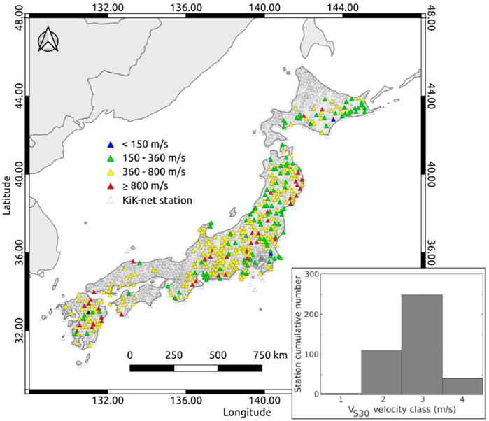
FIGURE 1. Map of KiK-net seismic stations (gray empty triangles) with colored triangles indicating selected seismic stations for the computation of SBSR and HVSRc subdivided into four V_S30 classes. In the inset, the histogram shows the number of stations in each class: 1. V_S30<150 m/s; 2.150≤V_S30<360 m/s; 3.360≤V_S30<800 m/s; 4. V_S30≥800 m/s.

Coda horizontal-to-vertical spectral ratio

The HVSRn is a fast and efficient method to obtain information on the local subsurface (SESAME, 2004; Rohmer et al., 2020; Panzera et al., 2022). However, this method is not directly applicable to KiK-net sites because we do not have access to continuous recordings (only pre-event signals) before the earthquake waveforms and because of the accelerometer sensor characteristics, which are not sensitive enough to low amplitude ambient vibration signals. In particular, the noise spectra measured at the sites are often even higher than the high noise model of Peterson (1993) (see e.g. in Figure 2). This is due to the KiK-net accelerometers, which have a high level of self-noise. For this reason, we explored alternative techniques to obtain an equivalent HVSRn. We applied the HVSR to the seismic coda waves (HVSRc), which were proven to satisfy the diffuse field assumption, and therefore, this allowed linking the HVSRc to HVSRn of the local structure (Margerin et al., 2009, 2000; Campillo and Paul, 2003; Sánchez Sesma et al., 2011).

FIGURE 2

FIGURE 2. Example of HVSRc computation at the station IBRH12. (A) A map showing the location of the site (black triangle) and the epicenters of the selected earthquakes (colored dots). (B,C) Power Spectral Density (PSD) in decibel for the noise (black lines) and for the earthquake recording on the vertical component (green lines) and horizontal mean component (blue lines), respectively. In the PSD graphs, the red lines are the Peterson (1993) high and low noise model boundaries. (D) SNR at the horizontal mean (blue lines) and vertical (green lines) component, as well as the number of earthquake spectra with SNR>3 as a function of frequency (red line). (E,F) shows the distribution of the HVSR on noise and on earthquake coda as a function of frequency. The color scale indicates the density of lines, each line corresponding to the HVSR of one single earthquake or noise window. In HVSR, the red lines indicate the mean and standard deviations.

The KiK-net database of the surface station recordings, covering the time period 1997–2020 (National Research Institute for Earth Science and Disaster Resilience, 2019), is used for the HVSRc computation. For the processing, P- and S-wave arrivals (T_P, T_S) were automatically detected by means of a time-frequency analysis; subsequently, the coda time was estimated as T_C=3.3T_S-2.3T_P following Perron et al. (2017). No restrictions on the hypocentral distance were imposed for the HVSRc estimation. For the HVSRc computation, as many as possible time windows are employed, comprised between T_C and the end of the signal; the time windows have a length of 25 s and a 50% overlap. A comparison between Fourier spectra (FAS) of coda and noise windows is performed by selecting noise between the beginning of the recording and T_P. This pre-event signal, used to compute FAS of noise in the KiK-net time series, has a variable duration, which is, on average, about 20 s. The Fourier Amplitude Spectrum Density (FASD) for the noise and for the coda windows were computed by normalizing by the square root of the respective window duration ($\sqrt{s}$), which allows a direct comparison of spectra with different durations. The horizontal mean FASD was then computed using the quadratic mean. The horizontal mean FASD was finally smoothed using the Konno and Ohmachi (1998) approach with a b-value of 80. The SNR of FASD was estimated by selecting only windows with SNR>3 over at least a two-octave frequency band window. The SNR is computed to select the FASD frequency band to use in the HVSRc computation for each considered earthquake. Therefore, for each earthquake, $\mathrm{H}\mathrm{V}\mathrm{S}\mathrm{R}\mathrm{c}$ was then obtained as the ratio between the horizontal mean FASD and the vertical FASD. Finally the between-events geometric mean and standard deviation at each frequency were computed. An example of computation is shown in Figure 2.

Unfortunately, it was not possible to assess the equivalence between HVSRc and HVSRn directly at the KiK-net stations. In fact, Figures 2B,C (black lines) shows that many of the noise spectra are characterized by the presence of high level of instrument self-noise, not allowing to compute reliable ambient vibration HVSRn. To our knowledge, a comprehensive database of ambient vibration recordings using sensitive seismometers is currently not available for the KiK-Net sites. Therefore, we tested the validity of the methodology on a set of 121 instrumented sites of the Swiss strong-motion network (SSMNet; Swiss Seismological Service, 1983). These sites are instrumented with accelerometers. During two successive phases of the SSMNet renewal (spanning 2009–2022), the stations’ sites have been the target of site characterization measurements aimed at reconstructing the local V_S profile by means of geophysical measurements, as well as retrieving the HVSR from single-station noise recordings to estimate the sites’ resonance frequencies (Michel et al., 2014; Hobiger et al., 2021). The ambient vibration recordings have been performed using portable velocimeter sensors and following the SESAME guidelines (SESAME, 2004). In particular, at all sites, the acquisition spans more than 30 min, and the measurement has been carried as close as possible to the station (with a maximum distance of 50 m). Acquired noise data has been processed following the SESAME guidelines and using a consistent procedure to compute HVSRn (i.e., using the same processing method and parameters). As anticipated, for each of these stations, the HVSRc was derived from earthquake coda data too, processing the strong-motion sensor recordings from earthquakes of the period 1998–2020 (SSMNet, doi:10.12686/sed/networks/ch) with the method illustrated above. We systematically collated HVSRc and HVSRn at each of the 121 stations (Figure 3). The agreement between the two HVSR curves is generally good (see examples in Figures 3A–D); globally, the frequency-by-frequency absolute distance between the two curves in log₁₀ scale is just below 0.2 log₁₀ units between 0.5 and 10 Hz in the 75% of cases (Figure 3E). The scale of these distances is comparable to that of the standard deviation across different time windows observed for the noise HVSR (σ_HVSRn), accounting for its variability. In Figure 3E, we report for comparison the frequency-dependent average standard deviations of HVSRn at all sites ($\overline{{\sigma }_{HVSRn}}$, continuous blue line), which decreases from about 0.2 log₁₀ units at 0.5 Hz (corresponding to the 75% cumulative value) to ∼0.1 log₁₀ units at 10 Hz (corresponding to the 50% cumulative value, i.e., the HVSRc—HVSRn distance is <0.1 in 50% of cases). Based on these systematic comparisons, we adopt the assumption that HVSR from coda data can be considered as virtually equivalent to the HVSR from ambient vibration recordings. We group the obtained HVSRc at KiK-net sites into four V_S30 classes (Figure 4) to highlight its wide range of geological and morphological conditions (from rock to soft soil).

FIGURE 3

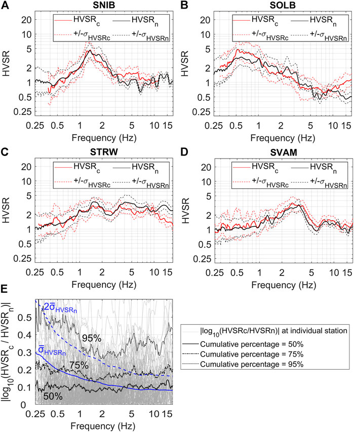
FIGURE 3. Collation between HVSRc and HVSRn at 121 Swiss strong-motion stations. HVSRn are obtained from field measurements of ambient noise acquired with velocimeters or from noise recorded by a co-located permanent seismometer. (A–D) Comparison between HVSRc and HVSRn at four sample stations; (E) overview of the global comparison HVSRc—HVSRn at all stations, expressed in terms of absolute differences between HVSRc and HVSRn on a log₁₀ scale. To understand the extent of these differences, the frequency-dependent average standard deviation observed at all HVSRn ($\overline{{\sigma }_{HVSRn}}$) is also plotted (blue lines).

FIGURE 4

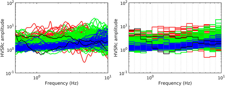
FIGURE 4. HVSRc (left panel) of the 428 selected seismic stations used in this study is subdivided into four V_S30 classes. In the right panel, HVSRc is subdivided into 16 frequency bins. The vertical dashed lines indicate the frequency bin limits, whereas the different colors refer to the four V_S30 classes used in this study. V_S30<150 m/s black lines; 150≤V_S30<360 m/s red lines; 360≤V_S30<800 m/s green lines; V_S30≥800 m/s blue lines.

Amplification functions dataset

For the computation of the SBSR, the events from the period 1997–2020 having a hypocentral depth ≤25 km and available at the NIED strong-motion portal (National Research Institute for Earth Science and Disaster Resilience, 2019) were used. This depth threshold is selected accordingly by Bergamo et al. (2022), who demonstrated that, after removing deep subduction earthquakes, the records exceeding the nonlinearity threshold of PGA = 0.1 g (Regnier et al., 2013) are a marginal fraction of the Japanese waveform database (≤1%). We can, therefore, assume that the computed amplification factors are largely determined by linear site response.

An automatic pick of P- and S-wave arrival times (T_P, T_S) by means of a time-frequency analysis (Perron et al., 2018) was performed. A signal window between T_P and 3.3T_S-2.3T_P and a noise window before T_P having almost the same duration as the signal window were selected. The signal window was also selected in a way that the top and bottom seismometer windows have the same length, taking the longest. The Fast Fourier Transform (FFT) for the noise and for the signal windows were computed, and the two horizontal components were averaged with a quadratic mean. The spectra were smoothed and resampled on a logarithmic scale using the Konno and Ohmachi (1998) approach with a b-value of 50. The SNR was also computed and only earthquakes with SNR>3 over at least a 10 Hz-wide frequency band both at the top and at the bottom seismometer were taken into account. The surface-to-borehole spectral ratio was then estimated for each selected earthquake, also estimating the between-events geometric mean and standard deviation at each frequency. SBSR was computed (Figure 5) for all the 428 KiK-net stations for which HVSRc is available (see previous section).

FIGURE 5

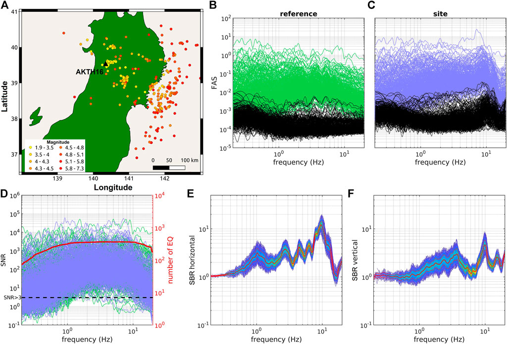
FIGURE 5. Example of surface-to-borehole spectral ratio at the station AKTH16. Panel (A) map showing the earthquake locations (colored dots) around the considered seismic station (black triangle); Panels (B,C) Fourier Amplitude Spectra (FAS) of the horizontal mean component for noise (black lines) and earthquake recordings at the bottom (reference) and top (site) seismometers. The FAS of the earthquake recordings are indicated by green lines at the bottom seismometer and blue lines at the surface seismometer. Panel (D) frequency-dependent SNR values for the reference (green lines) and the site (blue lines) seismometers. The red curve indicates the number of earthquakes used for each frequency value, whereas the horizontal dash line indicates the SNR threshold. Panel (E,F) SBSRs for horizontal and vertical components respectively.

When compared with SSR, the use of SBSR has the advantage of solving the between-station distance limitation but introduces some new difficulties due to the interaction of seismic waves within the subsurface. The interaction between up- and down-going waves is indeed fully constructive only at the soil surface, while it might be destructive at certain frequencies at depth (Thompson et al., 2009); furthermore, a damping effect during the propagation between surface and borehole receivers must be taken into account. These phenomena bias the estimation of the transfer function with reference to a standard outcrop rock site (Cadet et al., 2012a). Therefore, we implemented a correction procedure for the SBSRs, articulating into two successive steps. The first stage (termed depth correction) involves the correction for peculiar effects arising from the embedment of the borehole receiver in the subsurface (Kokusho and Sato, 2008; Cadet et al., 2012a, b; Tao and Rathje, 2020). In the second stage, the SBSRs are then referred to as the standard Japanese rock profile, as defined in Poggi et al. (2013). These two steps trace the procedure devised by Cadet et al. (2012a), for the same purpose.

Therefore, we first apply the depth correction, transforming SBSR into pseudo-SSR (pSSR), and then we correct pSSR to a common reference site with V_S30 of 1,350 m/s (Poggi et al., 2013), obtaining pseudo-empirical amplification functions (pEAF). Similarly to what has been done for HVSRc (Figure 4), to highlight the variability of the used amplification dataset, the obtained SBSR, pSSR, and pEAF are plotted into 4 V_S30 classes (Figure 6). In particular, the lowest V_S30 sites (black and red lines in Figure 6, V_S30 < 360 m/s) are clearly the sites with higher amplification, especially at low frequencies, whereas the highest V_S30 sites (blue lines in Figure 6, V_S30 ≥ 800 m/s) show almost flat amplification at low frequency with an increase at high frequency. The remaining sites (green lines in Figure 6, 360 ≤V_S30 < 800 m/s) display a behavior which is intermediate between soft sites and hard rock sites.

FIGURE 6

FIGURE 6. In the upper row mean SBSR (left panel), pSSR (central panel) and corresponding pEAF (right panel) of the 428 selected seismic stations used in this study subdivided in four V_S30 classes. In the lower row, SBSR (left panel), pSSR (central panel), and pEAF (right panel) are subdivided into 16 frequency bins. The vertical dashed lines indicate the frequency bin limits, whereas the different colors refer to the four V_S30 classes used in this study. V_S30<150 m/s black lines; 150≤V_S30<360 m/s red lines; 360≤V_S30<800 m/s green lines; V_S30≥800 m/s blue lines.

Canonical correlation

As shown in the previous section, from our earthquake data analysis we derived three different sets of amplification functions: SBSR, pSSR, and pEAF. Therefore, in the following description, the term AF (amplification function) is generically used to indicate one of these amplification sets.

The CC assesses the correspondence between two sets of variables X, Y identifying their best correlating linear combinations (Davis, 2002). In this study, the two sets of variables are the HVSRc and amplification functions (AF), both on a logarithmic scale, discretized within 16 frequency bins in the range of 0.50–10.00 Hz (Figures 4, 6). The bin subdivision used in this study is the same as in Panzera et al. (2021), who demonstrated that 16 bins are sufficient to preserve as much as possible of the HVSRc and AF fluctuations in amplitude. The average amplitude Am(k) within the kth bin is computed as a weighted mean,

$Am\left(k\right)=\frac{{\displaystyle \sum }_{l=\mathrm{1}}^{n_k}\left[\frac{A\left(f_{kl}\right)}{{\sigma }_{kl}^{\mathit{2}}}\right]}{{\displaystyle \sum }_{l=\mathit{1}}^{n_k}\left[\frac{\mathrm{1}}{{\sigma }_{kl}^{\mathit{2}}}\right]},k=\mathrm{1},n_{bin}(1)$

in which the weights are the inverse variances of HVSRc or AF on a logarithmic scale (${\sigma }^{\mathit{2}}$). In Eq. 1 $Am\left(f_{kl}\right)$ is the AF or HVSRc amplitude (in log scale) at the lth frequency $f_{kl}$ belongs to the kth frequency bin.. Following the CC procedure, the two groups of HVSRc (k=1, … ,n_bin) and AF (k=1, … ,n_bin) obtained from Eq. 1 are then transformed into the canonical variables X_can,i and Y_can,i,:

$\{\begin{array}{c}{X}_{can,i}={\displaystyle \sum }_{k=\mathrm{1}}^{n_{bin}}{b}_{k,i}\bullet \left[HVSRc\left(k\right)-\overline{HVSRc}\left(k\right)\right]\\ Y_{can,i}={\displaystyle \sum }_{k=\mathrm{1}}^{n_{bin}}{c}_{k,i}\bullet [AF\left(k\right)-\overline{AF}\left(k\right)]\end{array}(2)$

In Eq. 2, $\overline{AF}\left(k\right)$ and $\overline{HVSRc}\left(k\right)$ indicate the mean AF factor and mean HVSRc amplitude for the kth frequency bin, obtained by averaging over the entire population of sites. The CC determines as many i different couples of canonical variables as the minimum number of independent variables within each of the two input datasets; hence, in this study, the count of canonical couples is equal to the number of frequency bins (n_bin = 16) used for the discretization of HVSRc and AF_. The coefficients b_k,i and c_k,i of the linear transformations in Eq. 2 (named canonical loadings) are associated with the ith canonical couple (cc); in essence, every cc is identified by its own pair of vectors of canonical loadings b_i and c_i which maximize the correlation between X_can,i and Y_can,i (Figure 7A; more details in Davis, 2002).

FIGURE 7

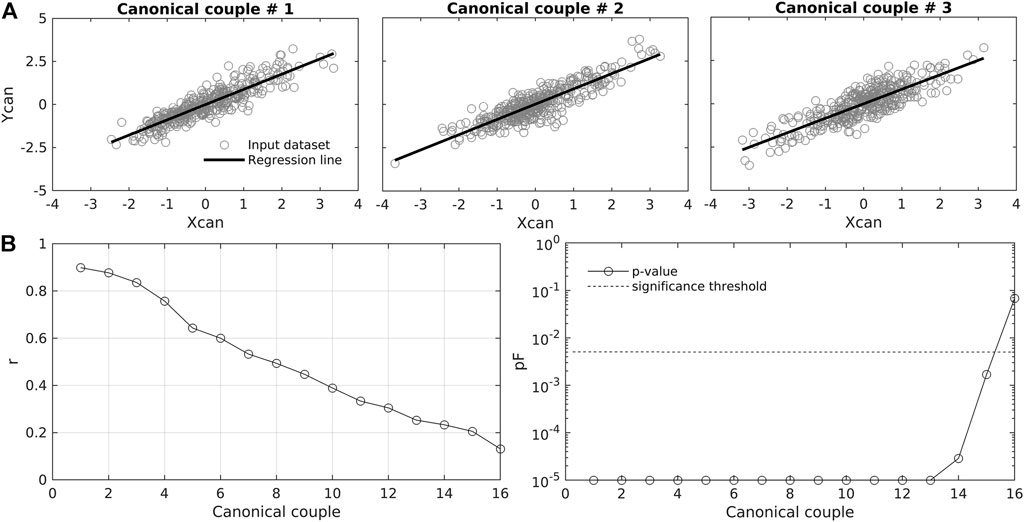
FIGURE 7. (A) Examples of first, second and third X_can—Y_can cc considering HVSRc and SBSR. Straight lines represent the linear regression between canonical variables. (B) cc vs. r coefficient (left panel) and cc vs. pF (right panel) graphs. Dashed black lines in the cc vs. pF graphs indicate the threshold value of 0.005.

The various cc stemming from the CC analysis are sorted according to decreasing values of the respective correlation coefficients between the variables X_can,i, - Y_can,i (r, Figure 7B, left panel). Each cc is also characterized by its own value of significance level for Rao’s scoring test (pF in Figure 7B, right panel; Rao 1973). The pF indicates the probability of erroneously stating that the canonical variables are related (Fisher, 1925), hence a small pF means that the correlation is reliable. We set 0.005 as the significance threshold for pF, as suggested by Benjamin et al. (2018). Consequently, taking into account this threshold for pF only the first 15 cc are significant, as shown in Figure 7B and considered to reconstruct the amplification functions.

To reconstruct the amplification from HVSRc, we used the approach proposed by Panzera et al. (2021). The method consists of solving the inverse problem for Eq. 2 (second line), i.e., retrieving AF_pred from Y_can with a least square (lsqr) approach with a regularization constraint (Tarantola, 2005).

${\mathrm{A}\mathrm{F}}_{pred}={\left({\mathrm{C}}^T{\mathrm{W}}^{-\mathrm{1}}\mathrm{C}\right)}^{-\mathrm{1}}{\mathrm{C}}^T{\mathrm{W}}^{-\mathrm{1}}{\mathrm{Y}}_{can}^{\prime }+\overline{\mathrm{A}\mathrm{F}}(3)$

where

4) AF_pred is the column vector of the unknown amplification values at the various frequency bins for the targeted prediction site, i.e. ${\mathrm{A}\mathrm{F}}_{pred}$(k = 1, … ,n_bin).

5) C is the matrix whose elements are the canonical loadings c_i,k (see Eq. 2) referring to the ith significant canonical couple (rows) and to the kth frequency bin (columns). To make the system of equations in 3 from under-to over-determined, n_bin-1 further rows are added to matrix C, incorporating a regularization constraint for AF_pred.

6) W is the diagonal matrix of weights containing along its main diagonal the coefficients of correlation r of each significant canonical couple (e.g., as in Figure 7B). For the extra rows of C incorporating the regularization constraint, a weight equal to ½ the minimum r is employed;

7) Y’_can is the column vector collecting the predicted canonical variables Y’_can for each of the n_cc significant canonical couples and referring to the targeted prediction site. Each element of Y’_can is a forecast for the actual realization of the variable Y_can for the ith cc, which is unknown as it is the linear combination of the unknown amplification factors at the various k=1, … , n_bin frequency intervals. Hence, we estimate Y’_can,i by first entering each ith canonical plane (Figure 7A) with the relevant X_can,i, which we retrieve with Eq. 2 as a linear transformation of the HVSRc obtained at the target site; Y’_can,i is then obtained as the ordinate of the point having abscissa = X_can,i along the linear regression line fitting the X_can, Y_can points of the calibration dataset (black lines in Figure 7A). Similarly, to C and W, Y_can is finally extended by adding n_bin-1 zeros corresponding to the regularization equations;

8) $\overline{\mathrm{A}\mathrm{F}}$ is the column vector of the mean amplification factors at each kth frequency bin over the whole population of the calibration sites.

More details on the preparation and description of the equation system [3] are reported in Panzera et al. (2021).

Modeling the AF from HVSR coda

We assess the prediction potential of the CC by using a leave-one-out cross-validation strategy: the CC system is calibrated on a set including all considered KiK-net sites but one, and a prediction for AF is attempted (with Eq. 3) for the site left outside the calibration ensemble. This operation is repeated as many times as the number of sites, performing the prediction for a different station every time. In Figure 8 we show examples of the ${AF}_{pred}$ computation for the seismic station AKTH07. From a visual inspection, the prediction of SBSRs and pSSRs is fairly good; however, a certain deviation from the target is instead observed when pEAF is predicted. As already noted by Panzera et al. (2021), this systematic deviation of ${AF}_{pred}$ with respect to the true amplification is observed when CC is applied to pEAF, which is referred to a common reference site, here defined by Poggi et al. (2013). The authors ascribed this effect to the fact that horizontal-to-vertical spectral ratios are fully site-dependent (i.e., not referred to a common reference), and hence their peak amplitude is influenced by the velocity contrast between the local bedrock and the surficial softer layers (Fäh et al., 2001; Bonnefoy-Claudet et al., 2006). To correct this deviation, Panzera et al. (2021) added to the CC a combination of site proxies (inferred or measured V_S30 and the thickness of ice cover at the last glacial maximum, the latter indirectly correlating with the stiffness of the present bedrock). In fact, in their study, a direct estimate of the shear wave velocity of the bedrock (V_S-bedrock) is not necessarily available at every seismic station.

FIGURE 8

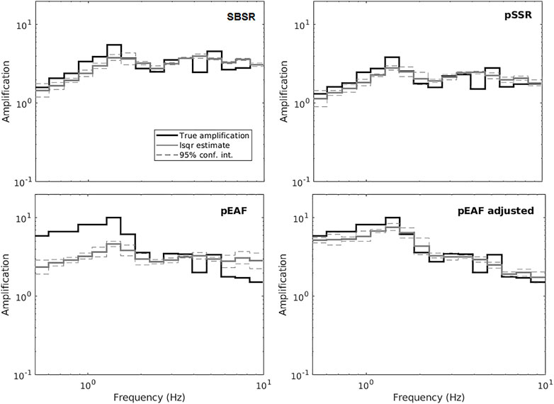
FIGURE 8. Comparison between true amplification and the ${AF}_{pred}$ at the station AKTH07 obtained by applying canonical correlation using HVSRc vs. SBSR, HVSRc vs. SSR, HVSRc vs. pEAF, and HVSRc plus V_S-bedrock vs. pEAF. The pEAF adjusted is referred to the prediction made by adding to the HVSRc matrix the column with the V_S-bedrock values.

In this study, we take advantage of the KiK-net velocity profiles, which reach the bedrock formation, to explore in more detail the influence of the local V_S-bedrock on the application of CC. In Figure 9, we then plot the V_S-bedrock of the sites versus the difference ${{\mathit{Log}}_{\mathrm{10}}(AF/AF}_{pred}$) obtained for each frequency bin. In general, it seems that when SBSR and SSR are predicted, ${{\mathit{Log}}_{10}(AF/AF}_{pred}$) always remains around 0 as a function of V_S-bedrock (Figures 9A,B). Instead, when pEAF is predicted, we observe a significant deviation of ${{\mathit{Log}}_{\mathrm{10}}(AF/AF}_{pred}$) towards values higher than 0 at low V_S-bedrock and lower than 0 at high V_S-bedrock (Figure 9C). This means that for low V_S-bedrock the ${AF}_{pred}$ prediction is underestimated, whereas at high V_S-bedrock the ${AF}_{pred}$ prediction is overestimated. In other words, when the local V_S-bedrock is lower than the velocity of the common reference site at the same depth, the prediction is underestimated and vice versa. The deviation from ${{\mathit{Log}}_{\mathrm{10}}(AF/AF}_{pred})=\mathrm{0}$ in Figure 9C can be explained in terms of the intrinsic nature of pEAF and HVSRc. In particular, the pEAF is referred to a common Japanese rock velocity profile (Poggi et al., 2013), while the HVSRc amplitude is controlled by the local velocity contrasts. Therefore, to correlate pEAF and HVSRc, this aspect should be taken into account. As additional proof, we finally add to the HVSRc matrix (collecting the predictor variables) a column with V_S-bedrock, to correct the observed deviation, and we visually observe an improvement in the prediction (Figure 8), also highlighted plotting ${{\mathit{Log}}_{\mathrm{10}}(AF/AF}_{pred}$) as a function of V_S-bedrock (Figure 9D). It is also to be considered that pEAF is derived from outcropping amplification functions referred to a common reference site. This procedure produces amplification functions that are not completely the same as the ones used by Panzera et al. (2021) and obtained by spectral modelling (Edwards et al., 2013). Probably during the two-steps procedure (Cadet et al., 2012a) used to derive pEAF, not all the effects are properly removed.

FIGURE 9

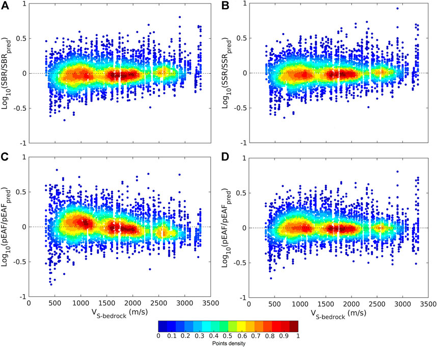
FIGURE 9. Scatterplots of V_S-bedrock vs. ${\mathit{Log}}_{\mathit{10}}\left({AF/AF}_{pred}\right)$ obtained using: (A) HVSRc and SBSR, (B) HVSRc and pSSR, (C) HVSRc and pEAF and (D) HVSRc plus V_S-bedrock and pEAF. The colored dots indicate individual seismic station values for each bin of frequency. The density of the points is indicated by the color scale of the dots, in particular warm colors indicate high density and cold colors indicate low point density. Dashed black line indicates ${\mathit{Log}}_{\mathit{10}}\left({AF/AF}_{pred}\right)=\mathit{0}$.

To determine the best combination of sets of variables to apply the canonical correlation, we additionally analyze the respective cumulative distributions of the mean errors per site ($∆$) at each station:

$∆=\frac{{\displaystyle \sum }_{k=\mathit{1}}^{n_{bin}}|{{\mathit{log}}_{\mathit{10}}(AF}_{pred}(k)){-\mathit{log}}_{\mathit{10}}(AF(k))}{n_{bin}}(4)$

The histograms in Figure 10 show that in general, the CC prediction works in a fairly good manner, with 80–85% of the sites having a ∆ below 0.2 (i.e., an average prediction error approximately within -50% to +50%). In more details, inspecting the corresponding cumulative distribution function (CDF), we observe a drastic change in the curves at about 85%. In particular, about 85% of the considered sites used in this study are predicted with $∆\le \mathit{0.15}$ when pSSR or pEAF is inferred by adding V_S-bedrock to the set of predictor variables. Instead, for the prediction of SBSR and pEAF, the 85th percentile increases to about 0.18. This means that our prediction accuracy decreases when we try to predict SBSR and pEAF only using HVSRc.

FIGURE 10

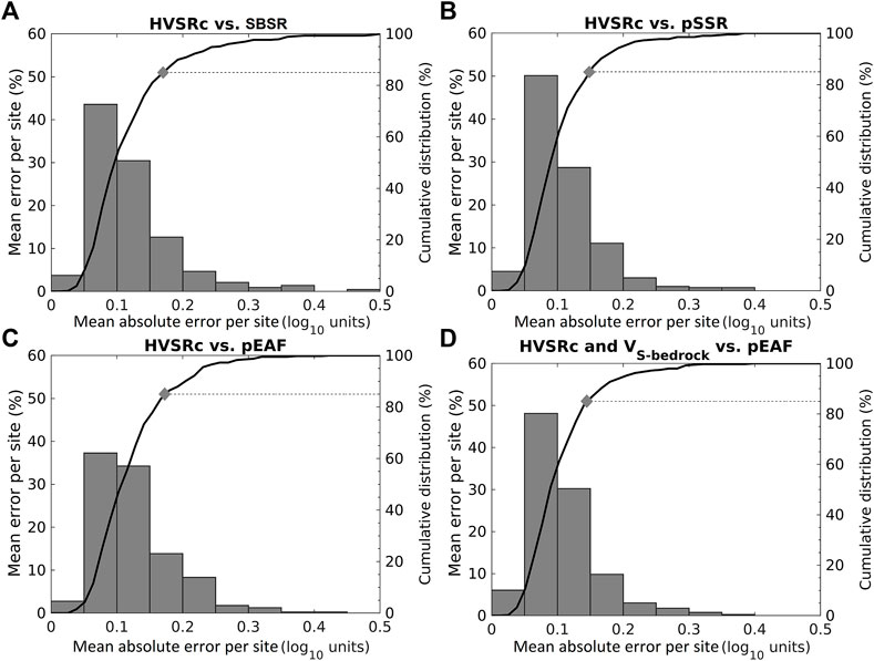
FIGURE 10. Histograms of the $∆$ per site obtained using: (A) HVSRc and SBSR, (B) HVSRc and pSSR, (C) HVSRc and pEAF and (D) HVSRc plus V_S-bedrock and pEAF. In the same graph, the black curves represent the corresponding cumulative distribution functions (CDF). Dashed lines and gray rhombus are used to highlight the $∆$ values corresponding to 85% of the CDF.

In all the CC analyses performed using a combination of AF and HVSRc, there are sites where the prediction is poor or fails. To determine for AF the number of bad predictions, we used the ∆=0.15 threshold obtained when CC is made using HVSRc and pSSR or HVSRc + V_S-bedrock and pEAF. This means that in our study we consider a prediction having $∆\le \mathit{0.15}$ (i.e. approximately comprised between −35% and +35%) as acceptable. Therefore, we count 77 (20.5%), 66 (17.6%), 102 (27.2%), and 62 (16.5%) poor or incorrect predictions from the CC analyses correlating HVSRc and SBSR, HVSRc and pSSR, HVSRc and pEAF, and HVSRc + V_S-bedrock and pEAF, respectively. Among the poor or incorrect predictions, 39 sites are common to all the CC analyses we carried out. For these sites, a possible explanation for the wrong prediction could be related to the position of the bottom seismometer, which doesn’t reach the “real” bedrock formation, i.e., the formation responsible for the fundamental resonance peak. An example of this situation is given in Figure 11 by the station EHMH04. At this site, a low frequency peak (<1.0 Hz) is present in the HVSRc, which cannot be modelled in the amplification function obtained by using SBSR. This means that below the borehole bottom seismometer, a significant velocity contrast could be present. This problem can be avoided by using EAF directly derived from empirical spectral modelling as in Panzera et al. (2021).

FIGURE 11

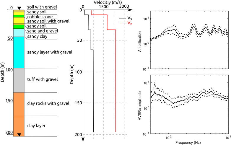
FIGURE 11. Soil column with related V_P and V_S profiles (modified from http://www.kyoshin.bosai.go.jp), SBSR and HVSRc for the station EHMH04. The black triangle in the soil column indicates the seismometer locations.

The remaining wrong predictions can be instead explained either in terms of local bedrock velocity influence (especially for pEAF) or in terms of up-going and down-going waves which can be destructive at certain frequencies at depth (especially for SBSR). Moreover, a not negligible effect could be played by peculiar lithologic and morphological settings, as in the cases of slopes, hills, high velocity rock sites, or deep basins.

We also verified the ${AF/AF}_{pred}$ distribution obtained from all the predictions in each considered frequency bin (Figure 12). The median value is always close to 1 and in general the ratio is in between 0.7–1.3 considering the 25th and 75th percentile, showing a significant improvement when pSSR and pEAF (using HVSRc plus V_S-bedrock) are predicted (Figures 12B,D). All the predicted AF shows progressive deviation from the true amplification at high frequencies, which becomes more evident above 5.22 Hz. A possible explanation could be that our dataset of amplifications and related HVSRc is characterized by an increase in variability moving from low to high frequencies (see Figure 12A). This aspect probably affects the uncertainty of the predictions (see for instance, AF and HVSRc of sites with V_S30> 800 m/s in Figures 4, 6). This means that besides the site-specific uncertainties (AF and HVSRc standard deviation) on the overall prediction of the amplification, single-site variability at each frequency bin of the overall dataset plays an important role.

FIGURE 12

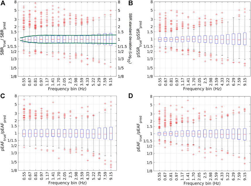
FIGURE 12. Box plot of the ${AF/AF}_{pred}$ distribution in each of the 16 frequency bins obtained using: (A) HVSRc and SBSR, (B) HVSRc and pSSR, (C) HVSRc and pEAF, and (D) HVSRc + V_S-bedrock and pEAF. The red lines are the median errors, the bottom and the top edges of the blue boxes are the 25^th and 75^th percentiles. The whiskers extend to the most extreme data points, excluding outliers represented as red crosses. The green lines in (A) are the average plus and minus standard deviations of the SBR dataset.

Adjustment factors for pEAF prediction

Site amplification is often referred to as a standard rock site for applications at a regional or national level. For this reason, we tested an alternative method to predict pEAF from CC as close as possible to the observed amplification. For instance, Panzera et al. (2021) in Switzerland added to the CC the V_S30 and the thickness of ice cover at the last glacial maximum. Here we observe that the best site proxy to add in CC when pEAF is used is the V_S-bedrock, but not always this information is available. Therefore, we tried to derive an equivalent value by using easily measurable site proxies such as V_S30, f₀ (HVSRc fundamental frequency), and A₀ (HVSRc amplitude of f₀). As f₀ we first identified the peak with the highest amplitude and then we adjusted by comparing with SBSR. This last comparison is made to be certain that picked f₀ is related to resonance between soil and the last layer in the logging in which the bottom sensor is located (Figure 13).

FIGURE 13

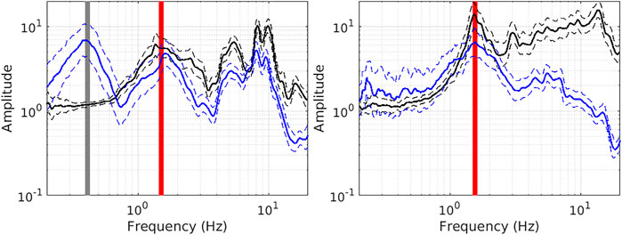
FIGURE 13. Comparison between SBSR (black line) and HVSRc (blue line) at two KiK-net seismic stations, FKSH11 (left panel) and KMMH03 (right panel). The automatic grey line indicates the first automatic piking, whereas the red line is the adjusted one after comparison with SBSR to be in agreement with resonance between soil and the last layer in the logging. If no grey line is displayed, no adjustment is necessary, as in the case of KMMH03 station.

In a simplified situation, the level of amplification, A is linked to the impedance contrast soil-bedrock through the following equation:

$A\approx \frac{{{\rho }_{bedrock}V}_{S-bedrock}}{\overline{{{\rho }_{soil}V}_S}}(5)$

where $\overline{V_S}$ is the average shear wave velocity of the sediment above the bedrock, ${\rho }_{bedrock}$ and $\overline{{\rho }_{soil}}$are the bedrock and average soil density, respectively. The $V_{S-bedrock}$ can be, then, retrieved from

$V_{S-bedrock}^{est}=\frac{\overline{{{\rho }_{soil}V}_S}}{{\rho }_{bedrock}}A(6)$

For each KiK-net velocity profile, we first computed ${\rho }_{bedrock}$ and ${\rho }_{soil}$ from the logging $V_P$ values by the Nagashima and Kawase (2021) equation:

$\rho =\mathrm{1.56}+1.86V_P{\mathrm{10}}^{-\mathrm{4}}(7)$

Moreover, the average $\overline{V_S}$ and the average $\overline{{\rho }_{soil}}$ for the soil cover above the bedrock were obtained using

$\overline{Z}=\frac{{\displaystyle \sum }_{i=\mathrm{1}}^n{h}_i}{{\displaystyle \sum }_{i=\mathrm{1}}^n\frac{h_i}{Z_i}}(8)$

where h is the thickness and Z is either ${\rho }_{soil}$ or $V_S$of the layer. To estimate the bedrock velocity is necessary to have an estimate of the $\overline{V_S}$, A and $\frac{\overline{{\rho }_{soil}}}{{\rho }_{bedrock}}$. As concerns the $\frac{\overline{{\rho }_{soil}}}{{\rho }_{bedrock}}$, we approximate it to an average value of 0.92 ± 0.06, considering all the sites in our dataset. For the $\overline{V_S}$ we instead derived a relationship between V_S30 and $\overline{V_S}$ is (Figure 14A)

${\mathit{log}}_{\mathrm{10}}\left(\overline{V_S}\right)=\mathrm{0.89}{\mathit{log}}_{10}\left(V_{S\mathrm{30}}\right)+\mathrm{0.45}(9)$

FIGURE 14

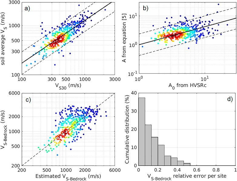
FIGURE 14. (A) Scatterplots of V_S30 vs. $\overline{V_S}$ in which the black line is the best fit line for equation [9]. (B) Scatterplots of A₀ vs. A in which the black line is the best fit line for equation [10]. (C) Scatterplots of $V_{S-bedrock}^{est}$ vs. V_S-bedrock from equation [11] in which dashed black line indicates $\mathit{1}:\mathit{1}\mathrm{r}\mathrm{a}\mathrm{t}\mathrm{i}\mathrm{o}$. (D) Histogram showing the distribution of the V_S-bedrock relative error per site. The dashed lines in (A–C) are the best fit lines and their 95% confidence intervals. The density of the points is indicated by the color scale of the dots (same as in Figure 9).

We also verified the equivalence between A, estimated using equation [5], and A₀ observing that A₀ is almost larger than A (Figure 14B). This behavior was already observed by Bonnefoy-Claudet et al. (2008), who observed that the HVSR peak always overestimates theoretical site amplification due to surface wave contributions. In particular, we found the following equation:

${\mathit{log}}_{\mathrm{10}}\left(A\right)=\mathit{0.63}{\log }_{10}\left(A_{\mathit{0}}\right)(10)$

Therefore, combining equation (9) and (10), we can estimate $V_{S-bedrock}^{est}$ by the following equation:

$V_{S-bedrock}^{est}=\mathrm{0.92}\ast {\mathrm{10}}^{\mathrm{0.89}{\mathit{log}}_{\mathrm{10}}\left(V_{S\mathrm{30}}\right)+\mathrm{0.45}}\ast {\mathrm{10}}^{\mathrm{0.63}{\log }_{\mathrm{10}}\left(A_{\mathrm{0}}\right)}(11)$

The $V_{S-bedrock}^{est}$ obtained from Eq.11 is plotted versus $V_{S-bedrock}$ in Figure 14C, in which the dots are quite well distributed along the 1:1 line. We also checked our results by plotting the relative error per site in the estimate of $V_{S-bedrock}$, obtained as the logarithm in base 10 of the ratio between estimated and true $V_{S-bedrock}$ (Figure 14D). From this plot, it is possible to verify that about 37% of the sites have an estimated $V_{S-bedrock}$ with an error of less than 15% (0.06 in log10 scale) and about 60% with an error less than 34% (0.13 in log10 scale). The biggest discrepancies in the estimate are observed for about 25% of the sites, with an error of more than 50% (0.13 in log10 scale). For these sites, the worst estimate is probably due to the fact that, although we adjusted the f₀ (see Figure 13), the used A₀ is not always related to the resonance between soil and bedrock, but to something shallower or deeper. Moreover, several authors debated the reliability of some KiK-net velocity profiles (Poggi et al., 2017; Pilz and Cotton, 2019).

Therefore, we performed several tests combining indirect and direct proxies to predict pEAF using CC. Among the indirect proxies we tested the Bouger anomalies, sediment thickness, and bedrock formation for Japan (Balmino et al., 2012; SDGM, 2014; Pelletier et al., 2016). As concern direct proxies we used V_S30, f₀, A₀, H800 and $V_{S-bedrock}^{est}$. From all the combinations, the best results were obtained using $V_{S-bedrock}^{est}$ or A₀, V_S30 and H800 (Figures 15A,B). The prediction in both cases improves, but we are not able to reach the high performance obtained using in the CC the true V_S-bedrock (Figure 15C). The V_S-bedrock of the sites versus the difference ${{\mathit{Log}}_{\mathrm{10}}(AF/AF}_{pred}$) tends to become parallel to 0 more when $V_{S-bedrock}^{est}$ is used (Figures 15D,E).

FIGURE 15

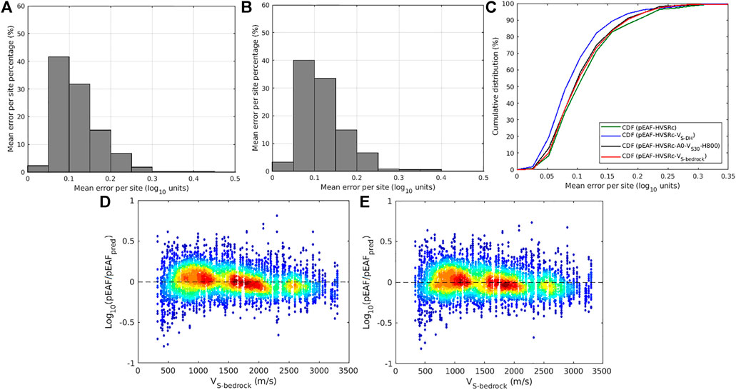
FIGURE 15. Histograms of the $∆$ per site obtained using: (A) HVSRc plus A₀, V_S30 and H800 and pEAF, (B) HVSRc plus $V_{S-bedrock}^{est}$ and pEAF, (C) cumulative distribution functions (CDF) comparison. Scatterplots V_S-bedrock vs. ${\mathit{Log}}_{\mathit{10}}\left({AF/AF}_{pred}\right)$ obtained using: (D) HVSRc plus A₀, V_S30 and H800 and pEAF and (E) HVSRc plus $V_{S-bedrock}^{est}$ and pEAF. The colored dots indicate individual seismic station values for each bin of frequency. The density of the points is indicated by the color scale of the dots (same as in Figure 9). Dashed black line indicates ${\mathit{Log}}_{\mathit{10}}\left({AF/AF}_{pred}\right)=\mathit{0}$.

Concluding remarks

In this work, the relationship between different types of amplification representations (SBSR, pSSR, and pEAF) and HVSRc was investigated through CC analysis using a large dataset derived from the KiK-net network. We computed HVSRc and SBSR at 428 seismic stations, deriving from the latter pSSR and pEAF. The equivalence between HVSRc and HVSRn was tested on Swiss strong-motion (SSMnet) sites, as to our knowledge, a database of ambient vibration recordings for KiK-net is not available. The agreement between the two kinds of HVSR curves is generally good, leading us to replace HVSRc in the CC for Japanese sites. The correlation between HVSRc and the various kinds of AFs was then performed using CC. The Panzera et al. (2021) technique based on a least square estimation method including a regularization constraint was used for the back computation of the amplification for the considered sites. The best correlation is obtained when SSR and HVSRc are used, whereas a strong deviation from empirical amplification is obtained when the pEAF is back computed. This deviation was already observed by Panzera et al. (2021) and explained in terms of the intrinsic nature of pEAF and HVSRc. In particular, the pEAF is normalized to the Japanese rock velocity profile defined in Poggi et al. (2013), while the HVSRc is affected by the local velocity contrasts. Therefore, taking advantage of the velocity profiles of the KiK-net stations, we demonstrate that, as assumed by Panzera et al. (2021), the best adjustment factor for CC when pEAF is used is the velocity of the bedrock. We also observed that a direct correlation between SBSR And HVSRc is possible, but the influence of the up-going and down-going waves, which are destructive at certain frequencies at depth, although not so evident, may play a role. Moreover, the wrong prediction in some cases is also related to the position of the bottom seismometer, which doesn’t reach the real bedrock formation. Such effects can be avoided if EAFs are directly derived, for instance, from empirical spectral modelling as in Panzera et al. (2021). A progressive deviation from the true amplification at high frequencies, which became more evident above 5.22 Hz, was observed. This aspect highlights that, in the overall prediction, the amplification site-to-site variability at each frequency bin of the overall dataset plays an important role. Finally, alternative methods were tested to predict site amplification referred to a generic rock site. In particular, we suggest using in the CC either a bedrock velocity estimated from HVSRc amplitude and V_S30 or a combination of A₀, V_S30 and H800. In particular, the $V_{S-bedrock}^{est}$ can be considered quite a robust estimate of the velocity of the bedrock, although it is strongly related to possible A₀ variability and to the considered site f₀.

In conclusion, canonical correlation has now been tested in different countries (Switzerland and Japan) with different datasets. Although some of the CC input datasets show some limitations when pEAF is used, it can provide quite a good estimate of the site amplification over selected frequency bins. The next step is to make the CC approach universal by preparing an extensive homogeneous dataset of SSR and HVSRn, for instance, starting from the 75 worldwide sites already chosen by Cultrera et al. (2014).

Data availability statement

The raw data supporting the conclusion of this article will be made available by the authors without undue reservation.

Author contributions

Concept and design of the study: FP, PB, and DF; acquisition of data: FP, VP, and PB; analysis and interpretation: FP, VP, and PB; drafting the manuscript: FP, VP, and PB; and revising critically for important intellectual content: DF. All authors approved the version of the manuscript to be published.

Funding

This work was conducted in the frame of the Earthquake Risk Model for Switzerland project, financed by contributions from the Swiss Federal Office for the Environment (FOEN), the Swiss Federal Office for Civil Protection (FOCP), and the Swiss Federal Institute of Technology Zurich (ETHZ). Open access funding provided by ETH Zurich.

Conflict of interest

The authors declare that the research was conducted in the absence of any commercial or financial relationships that could be construed as a potential conflict of interest.

Publisher’s note

All claims expressed in this article are solely those of the authors and do not necessarily represent those of their affiliated organizations, or those of the publisher, the editors, and the reviewers. Any product that may be evaluated in this article, or claim that may be made by its manufacturer, is not guaranteed or endorsed by the publisher.

References

Aoi, S., Kunugi, T., Nakamura, H., and Fujiwara, H. (2011). “Deployment of new strong-motion seismographs of K-NET and KiK-net,” in Earthquake data in engineering seismology: Geotechnical, geological, and earthquake engineering. Editors S. Akkar, P. Gülkan, and T. van Eck (Dordrecht: Springer), 14, 167–186.

CrossRef Full Text | Google Scholar

Balmino, G., Vales, N., Bonvalot, S., and Briais, A. (2012). Spherical harmonic modelling to ultra-high degree of Bouguer and isostatic anomalies. J. Geod. 86, 499–520. doi:10.1007/s00190-011-0533-4

CrossRef Full Text | Google Scholar

Benjamin, D. J., Berger, J. O., Johannesson, M., Nosek, B. A., Wagenmakers, E. J., Berk, R., et al. (2018). Redefine statistical significance. Nat. Hum. Behav. 2, 6–10. doi:10.1038/s41562-017-0189-z

PubMed Abstract | CrossRef Full Text | Google Scholar

Bergamo, P., Hammer, C., and Fäh, D. (2022). Correspondence between site amplification and topographical, geological parameters: Collation of data from Swiss and Japanese stations, and neural networks‐based prediction of local response. Bull. Seismol. Soc. Am. 112 (2), 1008–1030. doi:10.1785/0120210225

CrossRef Full Text | Google Scholar

Bergamo, P., Hammer, C., and Fäh, D. (2021). On the relation between empirical amplification and proxies measured at Swiss and Japanese stations: Systematic regression analysis and neural network prediction of amplification. Bull. Seismol. Soc. Am. 111 (1), 101–120. doi:10.1785/0120200228

CrossRef Full Text | Google Scholar

Bonnefoy-Claudet, S., Cornou, C., Bard, P. Y., Cotton, F., Moczo, P., Kristek, J., et al. (2006). H/V ratio: A tool for site effects evaluation. Results from 1-D noise simulations. Geophys. J. Int. 167, 827–837. doi:10.1111/j.1365-246x.2006.03154.x

CrossRef Full Text | Google Scholar

Bonnefoy-Claudet, S., Köhler, A., Cornou, C., Wathelet, M., and Bard, P.-Y. (2008). Effects of love waves on microtremor H/V ratio. Bull. Seismol. Soc. Am. 98 (1), 288–300. doi:10.1785/0120070063

CrossRef Full Text | Google Scholar

Boore, D. M. (2003). Simulation of ground motion using the stochastic method. Pure Appl. Geophys. 160, 635–676. doi:10.1007/pl00012553

CrossRef Full Text | Google Scholar

Borcherdt, R. D. (1970). Effects of local geology on ground motion near San Francisco Bay. Bull. Seismol. Soc. Am. 60 (1), 29–61.

Google Scholar

BSSC (2009). NEHRP recommended provisions for new buildings and other structures,” Part 1 (Provisions) and Part 2 (Commentary). Washington D.C: Federal Emergency Management Agency.

Google Scholar

Cadet, H., Bard, P.-Y., Duval, A. M., and Bertrand, E. (2012b). Site effect assessment using KiK‐net data: Part 2—site amplification prediction equation based on f0 and vsz. Bull. Earthq. Eng. 10, 451–489. doi:10.1007/s10518-011-9298-7

CrossRef Full Text | Google Scholar

Cadet, H., Bard, P.-Y., and Rodriguez‐Marek, A. (2012a). Site effect assessment using KiK‐net data: Part 1. A simple correction procedure for surface/downhole spectral ratios. Bull. Earthq. Eng. 10, 421–448. doi:10.1007/s10518-011-9283-1

CrossRef Full Text | Google Scholar

Campillo, M., and Paul, A. (2003). Long-range correlations in the diffuse seismic coda. Science 299 (5606), 547–549. doi:10.1126/science.1078551

PubMed Abstract | CrossRef Full Text | Google Scholar

Castro, R. R., Anderson, J. G., and Singh, S. K. (1990). Site response, attenuation and source spectra of S-waves along the Guerrero, Mexico subduction zone. Bull. Seismol. Soc. Am. 79, 1481–1503.

Google Scholar

Cen, (2004). Eurocode 8—design of structures for earthquake resistance—Part 1: General rules, seismic actions and rules for buildings. EN 1998-1. Brussels.

Google Scholar

Cultrera, G., De Rubeis, V., Theodoulidis, N., Cadet, H., and Bard, P.-Y. (2014). Statistical correlation of earthquake and ambient noise spectral ratios. Bull. Earthq. Eng. 12, 1493–1514. doi:10.1007/s10518-013-9576-7

CrossRef Full Text | Google Scholar

Davis, J. C. (2002). Statistics and data analysis in geology. 3rd edn. New York: Wiley.

Google Scholar

Derras, B., Bard, P. Y., and Cotton, F. (2017). V_S30, slope, H₈₀₀ and f₀: Performance of various site condition proxies in reducing ground-motion aleatory variability and predicting nonlinear site response. Earth Planets Space 69, 133. doi:10.1186/s40623-017-0718-z

CrossRef Full Text | Google Scholar

Di Giulio, G., Cultrera, G., Cornou, C., Bard, P. Y., and Al Tfaily, B. (2021). Quality assessment for site characterization at seismic stations. Bull. Earthq. Eng. 19, 4643–4691. doi:10.1007/s10518-021-01137-6

CrossRef Full Text | Google Scholar

Edwards, B., Michel, C., Poggi, V., and Fäh, D. (2013). Determination of site amplification from regional seismicity: Application to the Swiss national seismic networks. Seismol. Res. Lett. 84 (4), 611–621. doi:10.1785/0220120176

CrossRef Full Text | Google Scholar

Fäh, D., Kind, F., and Giardini, D. (2001). A theoretical investigation of averageH/Vratios. Geophys. J. Int. 145, 535–549. doi:10.1046/j.0956-540x.2001.01406.x

CrossRef Full Text | Google Scholar

Field, E. H., and Jacob, K. H. (1995). A comparison and test of various site-response estimation techniques, including three that are not reference-site dependent. Bull. Seismol. Soc. Am. 85 (4), 1127–1143.

Google Scholar

Fisher, R. A. (1925). Statistical methods for research workers, 43. Edinburgh, UK: Oliver & Boyd. ISBN 978-0-050-02170-5.

Google Scholar

Hobiger, M., Bergamo, P., Imperatori, W., Panzera, F., Lontsi, A. M., Perron, V., et al. (2021). Site characterization of Swiss strong-motion stations: The benefit ofadvanced processing algorithms. Bull. Seismol. Soc. Am. 111 (4), 1713–1739. doi:10.1785/0120200316

CrossRef Full Text | Google Scholar

Joyner, W. B., Warrick, R. E., and Fumal, T. E. (1981). The effect ofQuaternary alluvium on strong ground motion in the Coyote Lake, California, earthquake of 1979. Bull. Seismol. Soc. Am. 71, 1333–1349. doi:10.1785/bssa0710041333

CrossRef Full Text | Google Scholar

Kaklamanos, J., Baise, L. G., Thompson, E. M., Dorfmann, L., Kokusho, T., and Sato, K. (2015). Comparison of 1D linear, equivalent-linear, and nonlinear site response models at six KiK-net validation sites, Soil Dynamics and Earthquake EngineeringSurface-to-base amplification evaluated from KiK-net vertical array strong motion records. Soil Dyn. Earthq. Eng. 6928 (9), 207707–219716. doi:10.1016/j.soildyn.2007.10.016

CrossRef Full Text | Google Scholar

Kawase, H., Nagashima, F., Nakano, K., and Mori, Y. (2019). Direct evaluation of S-wave amplification factors from microtremor H/V ratios: Double empirical corrections to “Nakamura” method. Soil Dyn. Earthq. Eng. 126, 105067. doi:10.1016/j.soildyn.2018.01.049

CrossRef Full Text | Google Scholar

Konno, K., and Ohmachi, T. (1998). Ground motion characteristics estimated from spectral ratio between horizontal and vertical components of microtremor. Bull. Seismol. Soc. Am. 88, 228–241. doi:10.1785/bssa0880010228

CrossRef Full Text | Google Scholar

Margerin, L., Campillo, M., Van Tiggelen, A., and Hennino, R. (2009). Energy partition of seismic coda waves in layered media: Theory and application to pinyon flats observatory. Geophys. J. Int. 177, 571–585. doi:10.1111/j.1365-246X.2008.04068.x

CrossRef Full Text | Google Scholar

Margerin, L., Campillo, M., and Van Tiggelen, A. (2000). Monte Carlo simulation of multiple scattering of elastic waves. J. Geophys. Res. 105, 7873–7892. doi:10.1029/1999jb900359

CrossRef Full Text | Google Scholar

Michel, C., Edwards, B., Poggi, V., Burjanek, J., Roten, D., Cauzzi, C., et al. (2014). Assessment of site effects in alpine regions through systematic site characterization of seismic stations. Bull. Seismol. Soc. Am. 104, 2809–2826. doi:10.1785/0120140097

CrossRef Full Text | Google Scholar

Nagashima, F., and Kawase, H. (2021). The relationship between Vs, Vp, density and depth based on PS-logging data at K-NET and KiK-net sites. Geophys. J. Int. 225, 1467–1491. doi:10.1093/gji/ggab037

CrossRef Full Text | Google Scholar

Nakamura, Y. (1989). A method for dynamic characteristics estimation of subsurface using microtremor on the ground surface. QR RTRI 30 (1), 25–33.

Google Scholar

National Research Institute for Earth Science and Disaster Resilience (2019). NIED K-net, KiK-net. Tsukuba, Japan: National Research Institute for Earth Science and Disaster Resilience. doi:10.17598/NIED.0004

CrossRef Full Text | Google Scholar

Okada, Y., Kasahara, K., Hori, S., Obara, K., Sekiguchi, S., Fujiwara, H., et al. (2004). Recent progress of seismic observation networks in Japan-Hi-net, F-net, K-NET and KiK-net. Earth Planets Space 56. xv–xxviii. doi:10.1186/bf03353076

CrossRef Full Text | Google Scholar

Oth, A., Bindi, D., Parolai, S., and Di Giacomo, D. (2011). Spectral analysis of K-net and KIK-net data in Japan. Part II: On attenuation characteristics, source spectra, and site response of borehole and surface stations. Bull. Seismol. Soc. Am. 101 (2), 667–687. doi:10.1785/0120100135

CrossRef Full Text | Google Scholar

Panzera, F., Alber, J., Imperatori, W., Bergamo, P., and Fäh, D. (2022). Reconstructing a 3D model from geophysical data for local amplification modelling: The study case of the upper Rhone valley, Switzerland. Soil Dyn. Earthq. Eng. 155, 107163. doi:10.1016/j.soildyn.2022.107163

CrossRef Full Text | Google Scholar

Panzera, F., Bergamo, P., and Fäh, D. (2021). Canonical correlation analysis based on site‐response proxies to predict site‐specific amplification functions in Switzerland. Bull. Seismol. Soc. Am. 111 (4), 1905–1920. doi:10.1785/0120200326

CrossRef Full Text | Google Scholar

Pelletier, J. D., Broxton, P. D., Hazenberg, P., Zeng, X., Troch, P. A., Niu, G. Y., et al. (2016). A gridded global data set of soil, intact regolith, and sedimentary deposit thicknesses for regional and global land surface modeling. J. Adv. Model. Earth Syst. 8, 41–65. doi:10.1002/2015ms000526

CrossRef Full Text | Google Scholar

Perron, V., Gélis, C., Froment, B., Hollender, F., Bard, P.-Y., Cultrera, G., et al. (2018). Can broad-band earthquake site responses be predicted by the ambient noise spectral ratio? Insight from observation at two sedimentary basins. Geophys. J. Int. 215, 1442–1454. doi:10.1093/gji/ggy355

CrossRef Full Text | Google Scholar

Perron, V., Laurendeau, A., Hollender, F., Bard, P.-Y., Gélis, C., Traversa, P., et al. (2017). Selecting time windows of seismic phases and noise for engineering seismology applications: A versatile methodology and algorithm. Bull. Earthq. Eng. 16, 2211–2225. doi:10.1007/s10518-017-0131-9

CrossRef Full Text | Google Scholar

Peterson, J. (1993). Observations and modeling of background seismic noise, open-file report 93-322. Albuquerque, NM: U. S. Geological Survey.

Google Scholar

Pilz, M., and Cotton, F. (2019). Does the one-dimensional assumption hold for site response analysis? A study of seismic site responses and implication for ground motion assessment using KiK-net strong-motion data. Earthq. Spectra 35 (2), 883–905. doi:10.1193/050718eqs113m

CrossRef Full Text | Google Scholar

Poggi, V., Edward, B., and Fäh, D. (2017). A comparative analysis of site-specific response spectral amplification models. Phys. Chem. Earth Parts A/B/C 98, 16–26. doi:10.1016/j.pce.2016.09.001

CrossRef Full Text | Google Scholar

Poggi, V., Edwards, B., and Fäh, D. (2019). Development of hazard and amplification consistent elastic design spectra. Soil Dyn. Earthq. Eng. 126, 105118. doi:10.1016/j.soildyn.2018.03.011

CrossRef Full Text | Google Scholar

Poggi, V., Edwards, B., and Fäh, D. (2013). Reference S‐wave velocity profile and attenuation models for ground‐motion prediction equations: Application to Japan. Bull. Seismol. Soc. Am. 103 (5), 2645–2656. doi:10.1785/0120120362

CrossRef Full Text | Google Scholar

Rao, C. R. (1973). Linear statistical inference and its applications, Vol. 2. New York: Wiley.

Google Scholar

Régnier, J., Bonilla, L. F., Bard, P. Y., Bertrand, E., Hollender, F., Kawase, H., et al. (2018). Prenolin: International benchmark on 1D nonlinear site‐response analysis—validation phase exercise. Bull. Seismol. Soc. Am. 108 (2), 876–900. doi:10.1785/0120170210

CrossRef Full Text | Google Scholar

Régnier, J., Cadet, H., Bonilla, L. F., Bertrand, E., and Semblat, J. F. (2013). Assessing nonlinear behavior of soils in seismic site response: Statistical analysis on kik-net strong motion data. Bull. Seismol. Soc. Am. 103 (3), 1750–1770. doi:10.1785/0120120240

CrossRef Full Text | Google Scholar

Rohmer, O., Bertrand, E., Mercerat, E. D., Régnier, J., Pernoud, M., Langlaude, P., et al. (2020). Combining borehole log-stratigraphies and ambient vibration data to build a 3D Model of the Lower Var Valley, Nice (France). Eng. Geol. 270, 105588. doi:10.1016/j.enggeo.2020.105588

CrossRef Full Text | Google Scholar

Sánchez Sesma, F., Piña, J., Campillo, M., Luzón, F., García Jerez, A., Albarello, D., et al. (2012). “Seismic ambient noise H/V spectral ratio using the ACA (autocorrelations of coda of autocorrelations) approach,” in AGU fall meeting abstracts. S52C–04.

Google Scholar

Sánchez-Sesma, F., Rodríguez, M., Iturrarán-Viveros, U., Luzón, F., Campillo, M., Margerin, L., et al. (2011). A theory for microtremor H/V spectral ratio: Application for a layered medium. Geophys. J. Int. 186 (1), 221–225. doi:10.1111/j.1365-246x.2011.05064.x

CrossRef Full Text | Google Scholar

SDGM (2014). 1:200,000 seamless digital geological map of Japan (SDGM). Kasumigaseki, Chiyoda-ku, Tokyo: Geological Survey of Japan, National Institute of Advanced Industrial Science and Technology. Available at: https://gbank.gsj.jp/seamless/index_en.html?.

Google Scholar

SESAME (2004). Guidelines for the implementation of the H/V spectral ratio technique on ambient vibrations. Meas. Process. interpretation SESAME Eur. Res. Proj. deliverable D23.12.

Google Scholar

Swiss Seismological Service, , 1983. National seismic networks of Switzerland; ETH zürich. Other/Seismic Network. doi:10.12686/sed/networks/ch

CrossRef Full Text | Google Scholar

Tao, Y., and Rathje, E. (2020). The importance of distinguishing pseudo-resonances and outcrop-resonances in downhole array data. Bull. Seismol. Soc. Am. 110 (1), 288–294. doi:10.1785/0120190097

CrossRef Full Text | Google Scholar

Tarantola, A. (2005). Inverse problem theory and methods for model parameter estimation. Filadelfia, Pennsylvania, United States: Society for Industrial and Applied Mathematics, 348.

Google Scholar

Tchawe, F. N., Froment, B., Campillo, M., and Margerin, L. (2020). On the use of the coda of seismic noise autocorrelations to compute H/V spectral ratios. Geophys. J. Int. 220 (3), 1956–1964. doi:10.1093/gji/ggz553

CrossRef Full Text | Google Scholar

Thompson, E. M., Baise, L. G., Kayen, R. E., and Guzina, B. B. (2009). Impediments to predicting site response: Seismic property estimation and modeling simplifications. Bull. Seismol. Soc. Am. 99 (5), 2927–2949. doi:10.1785/0120080224

CrossRef Full Text | Google Scholar

Zhu, C., Pilz, M., and Cotton, F. (2020). Which is a better proxy, site period or depth to bedrock, in modeling linear site response in addition to the average shear-wave velocity? Bull. Earthq. Eng. 18, 797–820. doi:10.1007/s10518-019-00738-6

CrossRef Full Text | Google Scholar