Pre-quake frequency characteristics of Ms ≥7.0 earthquakes in mainland China

In this study, natural orthogonal expansion was performed on earthquake frequencies to compute the pre-quake frequency fields of 9 Ms ≥7.0 earthquakes in mainland China from 1980 to 2020. The temporal and spatial pre-quake anomalies of these earthquakes were extracted from their frequency fields. We found that the majority of pre-quake temporal anomalies (i.e., variations exceeding two-times the absolute mean square error) of a strong earthquake are condensed within the first four frequency fields, and typically comprise multiple components. The temporal factor of the first frequency field usually accounts for the largest proportion of these anomalies (40%–60% of the entire field). Most Ms ≥7.0 earthquakes exhibited long-term anomalies 5–8 years before their occurrence; some presented medium-term anomalies 1–2 years prior to the quake, and only a few presented short-term and imminent anomalies (≤3 months before the quake). Anomalous seismic hazard zones have high-gradient turning points in regional frequency-field contour maps, and the epicenters of strong earthquakes are often located in areas containing active faults that have contour values. Through the comparison of seismic frequency field and the traditional method of regional seismic activity frequency (3 months), it is shown that the frequency-field time factor has the advantages of diversified and rich abnormal information. The slope comparison between the frequency field and the cumulative frequency curve shows that the frequency anomaly time of the two is consistent, and the conclusion is reliable. Therefore, the seismic frequency method can predict the occurrence time and location of strong earthquakes, which is closer to the predictable seismic model.

1 Introduction

Before a strong earthquake there is an abnormal frequency of seismic activity around the source, wherein the frequency of seismic activity increases or decreases significantly compared with the normal level (Mei, 1996; Wyss and Habermann, 1998). Mogi (1969) studied the seismic activities around the focal area before the strong earthquake in Japan, and proposed for the first time that the frequency of earthquakes might increase or decrease significantly. Many subsequent studies have shown that there are frequent anomalous seismic signs around the focal points before most strong earthquakes, such as the 1988 Armenia Spitak Ms7.0 earthquake (Wyss and Habermann, 1998), 1992 US Landers Ms 7.3 earthquake (Wiemer and Wyss, 1994), 2011 Japan Ms 9.0 earthquake (Katsumata, 2011), 2014 Chile Iquique M_W 8.1 earthquake (Aden-Antoniow et al., 2020) and the 2015 Chile Illapel M_W 8.3 earthquake (Jarmolowski et al., 2021). Therefore, it is of great significance to study the abnormal variation characteristics of earthquake frequency for the development of earthquake prediction.

Some researchers have begun to study the anomaly of regional seismic activity frequency before strong earthquakes by using the traditional method of regional seismic variation over time. For instance, Feng et al. (2009) studied 22 moderate-to-strong earthquakes that occurred in the northeastern margin of the Qinghai–Tibet Block from 1980 to 2008, and found that 17 of these earthquakes were preceded by significant increases in the frequency of small earthquakes. Li et al. (2017) analyzed the data from the seismograph network around the Sichuan–Yunnan rhombic block and found significant anomalous increases in the local earthquake frequency prior to the 2013 Ms 7.0 Lushan Earthquake and 2014 Ms 6.5 Ludian Earthquake. This was an important result in terms of recognizing the precursors of strong earthquakes. Ma et al. (2008) studied the cumulative number of small earthquakes in the Qilian Mountain fault zone and variations in the earthquake frequency fields of Ms ≥6.0 earthquakes that occurred in China. Zhang and Li (2021) noted that the activity of small earthquakes around the focal point of the Maduo Ms 7.4 earthquake in Qinghai province increased significantly before the earthquake, and that the Luqu earthquake swarm was formed. They theorized that the Luqu area is a stress-sensitive area, which has a good corresponding relationship to the Maduo Ms 7.4 earthquake. Ma et al. (2022) studied 15 Ms ≥7.0 earthquakes in mainland China, and the cumulative frequency of earthquakes showed exponential growth. They found that at the annual scale non-linear growth characteristics are present in a cumulative number of small earthquakes before Ms ≥7.0 earthquakes. They also demonstrated that the gradient of the cumulative earthquake frequency graph changes prior to a moderate or strong earthquake owing to the formation of a seismogenic stress state in the region. The research methods of these scholars are effectively similar, in that they are one-dimensional images of earthquake frequency variable with time, which can predict the occurrence time of strong earthquakes.

The application of field theory to study anomalies before strong earthquakes is relatively new, having only been developed in recent years. The natural orthogonal expansion method (Ma et al., 1993) is used to calculate the energy field or frequency field before a strong earthquake. Two-dimensional images of the time and space of typical fields are studied, so as to predict the time and location of strong earthquakes. In particular, seismic energy fields have been studied intensively by several authors. For example, energy field theory was used for the first time by Yang and Ma (2004) to study how temporal anomalies in seismic energy are related to strong earthquakes in Ningxia. Luo and Yang (2005) conducted a systematic analysis of the relationship between spatial and temporal seismic energy field anomalies and moderate-to-strong earthquakes in Yunnan based on the seismic energy field in the region since 1975. Luo et al. (2011a) extracted spatiotemporal anomalies from the seismic energy field of the northwest Yunnan to south Yunnan region and accurately predicted the strong earthquakes that occurred in this region over the next 3 years. Luo et al. (2011b) and Yang and Ma (2011), Yang and Ma (2012) discovered medium- and short-term temporal and spatial anomalies in the seismic energy field of Wenchuan prior to the 2008 Ms 8.0 Wenchuan Earthquake that corresponded closely to the earthquake event. Ma and Yang (2012) analyzed the pre-quake temporal changes in the seismic energy field of the area around the epicenter of the 2010 Ms 7.1 Yushu Earthquake and the Yushu Fault and found that spatiotemporal energy-field anomalies preceded the earthquake by approximately half a year. Yang and Ma (2013) reviewed the pre-quake temporal factors of seismic activity fields around the epicenters of 30 Ms ≥6.0 earthquakes in China and found that most of these earthquakes were preceded by significant temporal anomalies. Luo et al. (2014) studied pre-quake spatiotemporal anomalies in the seismic energy field of the epicenter of the 2013 Ms 6.6 Minxian Earthquake and analyzed the correspondence between the evolution of spatiotemporal anomalies in the pre-quake seismic energy field and the epicenter of the Ms 6.6 earthquake. Yang et al. (2017) studied the strain fields of Ms ≥6.0 earthquakes in China and found that the temporal anomalies of such fields are more useful as earthquake predictors than those of seismic energy fields. Luo et al. (2018) studied the pre-quake seismic strain field of the 2017 Ms 7.0 Jiuzhaigou Earthquake and compared the temporal evolution of the strain anomalies of this earthquake with that of the 1976 Ms 7.2 Songpan–Pingwu Earthquake. Luo et al. (2019a) studied the pre-quake spatiotemporal anomalies of seismic strain fields around the epicenter of large earthquakes with an emphasis on their relationship to the mainshock. Luo et al. (2019b) studied how the seismic strain field of the Ms 8.0 Wenchuan Earthquake affected the subsequent Ms ≥6.0 earthquakes in the Longmenshan Fault and other nearby faults by investigating the interactions between strong earthquakes from the perspective of seismic strain evolution. Ma et al. (2020) applied a natural orthogonal function to study the variation of frequency field time factor of 7 Ms 7 earthquakes and 8 Ms 6 earthquakes and found that frequency field anomalies before strong earthquakes mainly concentrated in the first and second typical fields.

On the basis of the above research, we extracted the spatial isoline anomalies of the frequency field, studied the spatiotemporal abnormal variation characteristics of the frequency field of seismic activity before strong earthquakes in mainland China, and considered the abnormal variation rules of Ms ≥7.0 earthquakes. Next, through the comparison of seismic frequency field and the traditional method of regional seismic activity frequency (3 months), it was found that the frequency field time factor has the advantages of diversified and rich abnormal information. A slope comparison between the frequency field and the cumulative frequency curve then revealed that the frequency anomaly time of the two is consistent, and the conclusion is reliable. Lastly, the seismic frequency method was used to predict the occurrence time and location of strong earthquakes, and was found to be closer to the predictable seismic model.

2 Data and methods

2.1 Convolution regression method

The earthquake frequencies of a region are random variables that can be decomposed via natural orthogonal expansion into spatial and temporal functions. These functions comprise the earthquake frequency field, N. A random field can then be created by gridding the study area according to its local earthquake frequencies, that is, by dividing the study area, ∆N, into n elements of equal areas such that $∆N=∆x\times ∆y$. The central coordinates of each element are $\left({\mathrm{x}}_j,{\mathrm{y}}_j\right)\left(j=\mathrm{1,2},\dots ,n\right)$. The observation time, t_i, is then divided into m intervals of length $∆t$ such that $t_i=∆t\times I\left(i=\mathrm{1,2},\dots ,m\right)$. The observed seismic activity frequency of each element during each time interval is then calculated and recorded as N_ij; these values constitute the function field of the spatiotemporal coordinates $\left(x_i,y_i,t_j\right)\left(i,j=\mathrm{1,2},\dots ,n\right)$.

We herein express N, the frequency of the seismic activity applied in the gridding of the study area, as $N={\displaystyle \sum }_i{N}_{ij}$, which has the following matrix representation:

$N=\left[\begin{array}{cccc}{N}_{11}& N_{12}& \cdots & N_{1n}\\ N_{21}& N_{22}& \cdots & N_{2n}\\ ⋮& ⋮& ⋮& ⋮\\ N_{m1}& N_{m2}& \cdots & N_{mn}\end{array}\right],(1)$

where $N_{ij}\left(i=\mathrm{1,2},\dots ,m,j=\mathrm{1,2},\dots ,n\right)$ is the cumulative earthquake frequency of the j-th grid (spatial factor) during the i-th time interval (temporal factor). A natural orthogonal expansion is then performed on N by decomposing the matrix into the sum of the products of the orthogonal spatial functions x and orthogonal temporal functions T, that is,

$N_{ij}={\displaystyle \sum }_{p=1}^n{T}_{ip}{X}_{pj}\left\{\begin{array}{c}i=\mathrm{1,2},\cdots ,m\\ j=\mathrm{1,2},\cdots ,n\end{array}\right..(2)$

These functions are orthogonal and normalized and satisfy the conditions

${\displaystyle \sum }_{j=1}^n{x}_{kj}{x}_{lj}=\left\{\begin{array}{cc}0& k\ne l\\ 1& k=l\end{array}\right.,(3)$

${\displaystyle \sum }_{i=1}^m{T}_{ik}{T}_{il}=\left\{\begin{array}{cc}0& k\ne l\\ {\lambda }_k& k=l\end{array}\right..(4)$

We can then define the matrix $R=N’N$ and solve for the characteristic equation of R, that is,

$\left[\begin{array}{cccc}{R}_{11}& R_{12}& \cdots & R_{1n}\\ R_{21}& R_{22}& \cdots & R_{2n}\\ \cdots & \cdots & \cdots & \cdots \\ R_{n1}& R_{n2}& \cdots & R_{nn}\end{array}\right]\left[\begin{array}{c}{x}_1\\ x_2\\ \cdots \\ x_n\end{array}\right]=\lambda \left[\begin{array}{c}{x}_1\\ x_2\\ \cdots \\ x_n\end{array}\right],(5)$

from which we obtain the eigenvectors ${\stackrel{\rightharpoonup }{x}}_k$ and eigenvalues ${\lambda }_k\left(k=\mathrm{1,2},\dots ,n\right)$. The temporal factors can then be expressed as

$\begin{array}{cc}{\stackrel{\rightharpoonup }{T}}_k=N{\stackrel{\rightharpoonup }{x}}_k& k=\mathrm{1,2},\cdots n.\end{array}(6)$

The eigenvectors ${\stackrel{\rightharpoonup }{x}}_k$ (frequency field) represent the spatial distribution of earthquake frequencies in each field, and the temporal factor ${\stackrel{\rightharpoonup }{T}}_k$ represents the time dependence of the frequency field ${\stackrel{\rightharpoonup }{x}}_k$ as well as reflecting the dynamics of each time-frequency field. The eigenvectors corresponding to the first few eigenvalues of R (which are arranged in decreasing order) are sufficiently precise to fit the entire frequency field. In other words, we can approximate the entire frequency field by superimposing the first few eigenvectors (frequency fields), with the changes that occur in these first fields representing the spatiotemporal characteristics of the frequency field corresponding to the study area. If the sum of all n eigenvalues is $b_0$, the precision of fit between the first l frequency fields and the entire field is

$r_l={\displaystyle \sum }_{p=1}^l{\lambda }_p/b_0,(7)$

where ${\lambda }_{\mathrm{p}}$ is the p-th characteristic root.

In summary, natural orthogonal expansion condenses most of the information carried by an earthquake frequency field into the “primary” frequency fields that correspond to its largest eigenvalues. Frequency fields that are either invariant or poorly correlated with large quakes can then be excluded, thus simplifying the problem to the anomalies of the first few frequency fields.

2.2 Data and case examples

The earthquake data used in this study were obtained from the official national earthquake catalog provided by the China Earthquake Networks Center. The b-values of the study areas that correspond to the epicenters of 9 Ms ≥7.0 earthquakes were estimated from the earthquake catalog and their minimum magnitudes of completeness, Mc. One of the considerations in this study was the difference between frequency and energy fields. Small earthquakes (Ms 2-3) reflect the background seismicity of each region and have a significant effect on the earthquake frequency fields; large earthquakes, which are primarily controlled by seismogenic mechanisms, have a stronger effect on the energy field. To ensure that the selected dataset adequately reflected the background seismicity of a region as well as the seismogenic processes of large earthquakes, earthquakes between Mc and M_L 5.4 (Ms 5.0) were included in the dataset. In principle, the aftershocks of each study area should also be included in the dataset. However, for cases in which the study areas of Ms ≥7.0 earthquakes overlapped, it was necessary to eliminate the aftershocks of the earlier earthquake to avoid affecting the later earthquake. For example, the study areas of the 2008 Ms 8.0 Wenchuan Earthquake and 2013 Ms 7.0 Lushan Earthquake overlapped; in this case, it was necessary to omit the aftershocks of the Ms 8.0 Wenchuan Earthquake from the dataset. The grid was divided into square cells of 1.0°x1.0°, and the time interval was selected as 3 months. The data were discretized and calculated, and the specific spatiotemporal scale was discussed in the following paper. Earthquake frequency matrices, N, were constructed for each study area using Eq. 1. These matrices were then analyzed by natural orthogonal expansion and the corresponding R matrices were solved to obtain the eigenvalues of the frequency field, primary fields that correspond to these eigenvalues, temporal factors of these primary fields, and frequencies of the spatial grids of each study area.

Natural orthogonal expansion was used to analyze the pre-quake local frequency fields of all Ms ≥7.0 earthquakes in mainland China from 1980 to 2020 (Figure 1). However, based on Wang et al. (2017) studies of the disparities in the precision and sensitivity of the national seismograph network (especially in Tibet and parts of Qinghai, where the network is poorly developed), the seismic observation data of the following earthquakes were found to be insufficiently complete for the purposes of this study: the Ms 7.5 Earthquake in Mani, Tibet, on 8 November 1997; the Ms 8.1 earthquake to the west of the Kunlun Pass on 14 November 2001; and the Ms 7.1 earthquake in Yushu Tibetan Autonomous Prefecture on 14 April 2010. Therefore, the frequency fields of these earthquakes were not computed in this study.

FIGURE 1

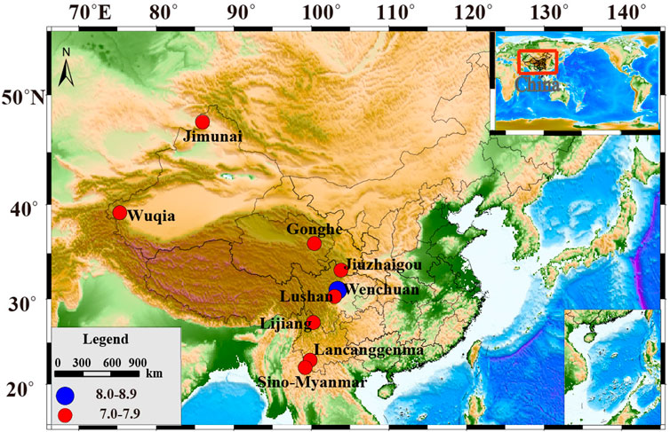
FIGURE 1. Locations of 9 Ms ≥7.0 earthquakes in mainland China. Red circles represent magnitude-7.0–7.9 earthquakes, and blue circles represent magnitude-8.0–8.9 earthquakes, the spatial distribution of epicenters in the Chinese mainland from 1980 to 2022.

2.3 Earthquake parameters and computational accuracy

The proposed method was first tested on the Ms 7.1 Wuqia Earthquake that occurred on 23 August 1985. The coordinates of its study area are (74.5°–77.5°E, 39°–41°N) and the b-value of this area was estimated using the seismic data from January 1975 to July 1985. The Mc of this area was determined to be M_L = 2.7 according to the G-R equation (Figure 2). The study area was divided into 1.0°×1.0°grids, with a time interval of ∆t = 1/4 years (3 months). The earthquake frequency field of the n grids (n = 6) and m time intervals (m = 42) was then computed. When l = 4, the first four frequency fields encompass 88.91% of the entire frequency field, which is equivalent to all of the pre-quake frequency field anomalies of the Ms 7.1 Wuqia Earthquake being condensed within these four primary frequency fields. In other words, the anomalies in the first four frequency fields were equivalent to all of the anomalies of the study area. The parameters of the other 8 Ms ≥7.0 earthquakes and their computed results are listed in Table 1. This table includes the selected earthquakes and their spatial and temporal ranges, the magnitudes of the weak earthquakes included in the frequency field, the number of computational grids and time intervals, the magnitudes of the first four eigenvalues, and the accuracy of fit between the first four frequency fields and the entire field. It is seen from the table that the study areas of most of the Ms ≥7.0 earthquakes were larger than 3°×3° and spanned ten years or more (Yang et al., 2017) except in a few special cases. For instance, the spatial and temporal ranges of the 2017 Ms 7.0 Jiuzhaigou Earthquake had to be selected in a different manner to account for the influence of the 2008 Ms 8.0 Wenchuan Earthquake. The accuracy of fit between the entire frequency field and first four frequency fields was always greater than 70%, and the fit was 100% for the 1988 Ms 7.6 Lancang–Gengma Earthquake. Therefore, most of the anomaly data carried by the earthquake frequency fields (regardless of location) have been condensed within the first four frequency fields, and the anomalies of the first four frequency fields are representative of all anomalies in the study areas. The temporal changes in the pre-quake frequency fields of the aforementioned earthquakes are shown in Figure 3. All changes in the temporal factors that were greater than two times the magnitude of the pre-quake mean square error were deemed to be anomalies. The anomalies were then classified as long-term, medium-term, short-term, or imminent anomalies and the primary frequency fields that induced these anomalies are identified in Table 2. These results served as a guide for subsequent comparisons between the pre-quake anomalies of each frequency field.

FIGURE 2

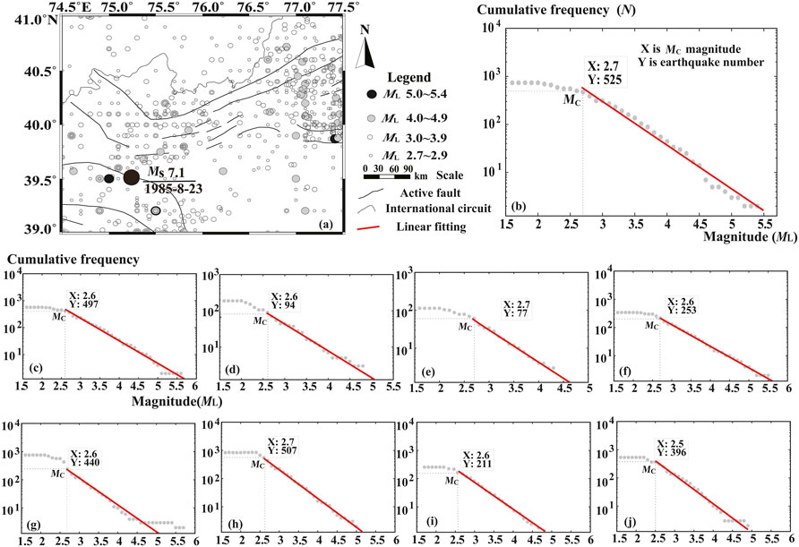
FIGURE 2. Spatial distribution of Ms 7.1 Wuxia earthquake epicenters, The gray circles represent earthquakes of magnitude 2.7 to 5.4 (A).The G-R relationship of 9 earthquake cases above Ms 7 in the study area, the gray dot represents the cumulative number of earthquakes, and the red line represents the linear fit (B–J). (B) 1985 Ms 7.1 Wuxia earthquake; (C) 1988 Ms 7.6 Lancang–Gengma earthquake; (D) 1990 Ms 7.0 Gonghe earthquake; (E) 1990 Ms 7.2 Jeminay earthquake; (F) 1995 Ms 7.3 Myanmar–China earthquake; (G) 1996 Ms 7.0 Lijiang earthquake; (H) 2008 Ms 8.0 Wenchuan earthquake; (I) 2013 Ms 7.0 Lushan earthquake; (J) 2017 Ms 7.0 Jiuzhaigou earthquake.

TABLE 1

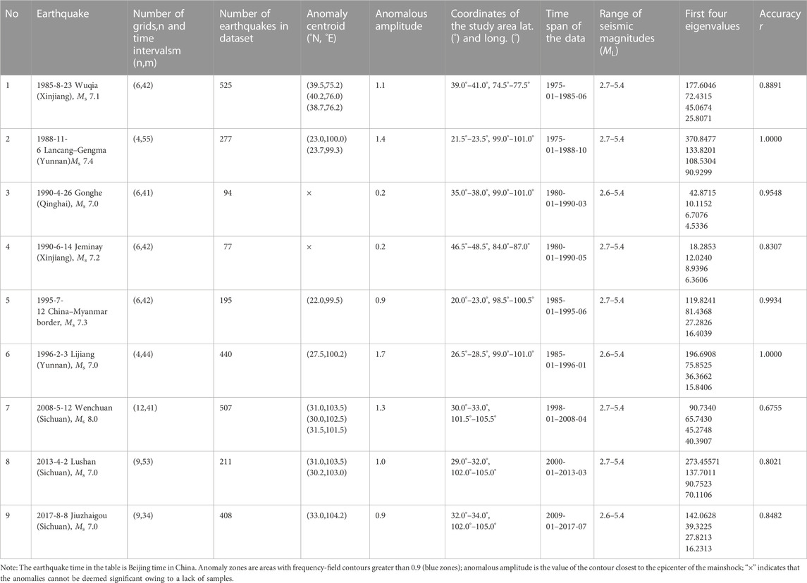
TABLE 1. Parameters and computed frequency fields of 9 Ms ≥7.0 Earthquakes in mainland China.

FIGURE 3

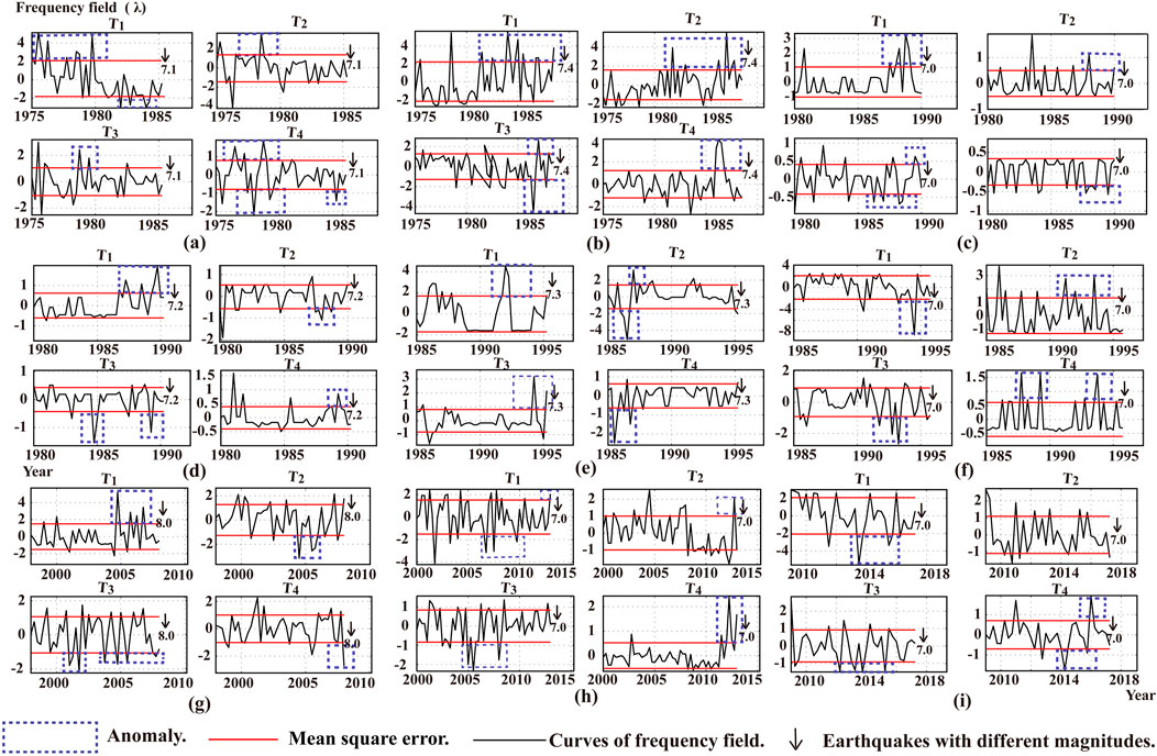
FIGURE 3. Temporal factors of the first four frequency fields of 9 Ms ≥7.0 earthquakes, The green dotted line represents the anomaly, The red line is two times the mean square error, The black arrow represents the magnitude of a Ms ≥7.0 earthquake. (A) 1985 Ms 7.1 Wuxia earthquake; (B) 1988 Ms 7.6 Lancang–Gengma earthquake; (C) 1990 Ms 7.0 Gonghe earthquake; (D) 1990 Ms 7.2 Jeminay earthquake; (E) 1995 Ms 7.3 Myanmar–China earthquake; (F) 1996 Ms 7.0 Lijiang earthquake; (G) 2008 Ms 8.0 Wenchuan earthquake; (H) 2013 Ms 7.0 Lushan earthquake; (I) 2017 Ms 7.0 Jiuzhaigou earthquake.

TABLE 2

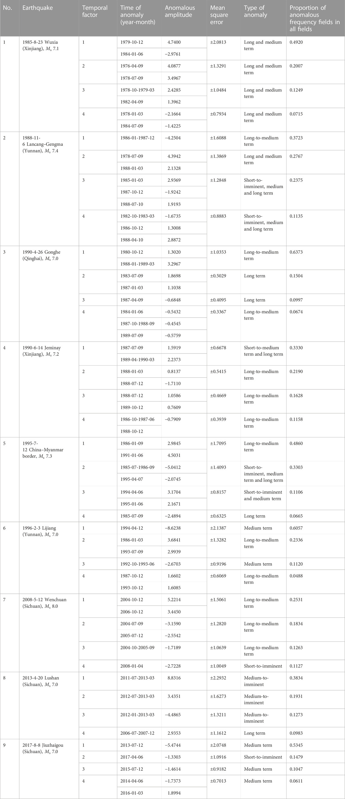
TABLE 2. Parameters of the frequency field temporal factors of 9 Ms ≥7.0 earthquakes in mainland China.

2.4 Changes in temporal factors of the frequency fields

The temporal factor anomalies that appeared in the frequency fields of the 9 Ms ≥7.0 earthquakes shown in Table 2 reveal that, in each of these earthquakes, the temporal factors of the first four frequency fields (T₁–T₄) exhibited one or more anomalies at different times. For each earthquake, the anomalous amplitude is taken as the largest value between several consecutive anomalies, and a change is deemed anomalous if it is larger than twice the absolute mean square error. Under the earthquake forecasting standards of the China Earthquake Administration, anomalies that appear 10 years, 1–2 years, 3 months, and a few to tens of days before a mainshock are called long-term, medium-term, short-term, and imminent anomalies, respectively. The vast majority of the 9 Ms ≥7.0 earthquakes exhibited long-term and medium-term anomalies, such as the 2008 Ms 8.0 Wenchuan and 2013 Ms 7.0 Lushan Earthquakes, and also showed short-term and imminent anomalies. Overall, the T₁–T₄ graphs of the Ms ≥7.0 earthquakes always exhibit large and complex fluctuations and contain many anomalies that exceed the anomaly determination threshold (the range of the mean square error is indicated by red lines in Figure 3). Some of these earthquakes exhibited extremely significant imminent anomalies, which are useful as earthquake predictors.

2.5 Changes in contours of frequency fields

The frequency-field contour maps of the areas that correspond to the 9 Ms ≥7.0 earthquakes that occurred in mainland China from 1980 to 2020 are shown in Figure 4. These maps were computed using Eq. 6 based on the weak-earthquake data described in Table 1. It is seen that the locations of the mainshocks coincide with high-density gradient turning points (locations where the blue zones turn into red zones, which have gradients greater than 0.9) in seven out of the nine earthquakes. The mainshocks typically occur near the turning points rather than the maximum contour values. In two other earthquakes (the 1990 Ms 7.0 Gonghe Earthquake and Ms 7.2 Jimenay Earthquake), the contours are relatively sparse and small in number and do not exhibit any significant anomalies. This is potentially related to the low earthquake monitoring ability and low earthquake frequency in the study area. Generally, high-gradient turning points appear when the values of the frequency-field contour lines become large, and an area can exhibit one or more of these anomalous zones. Anomalous zones that occur near an active fault are often the epicenters of Ms ≥7.0 earthquakes; other anomalous zones can become the epicenter of strong earthquakes in the future.

FIGURE 4

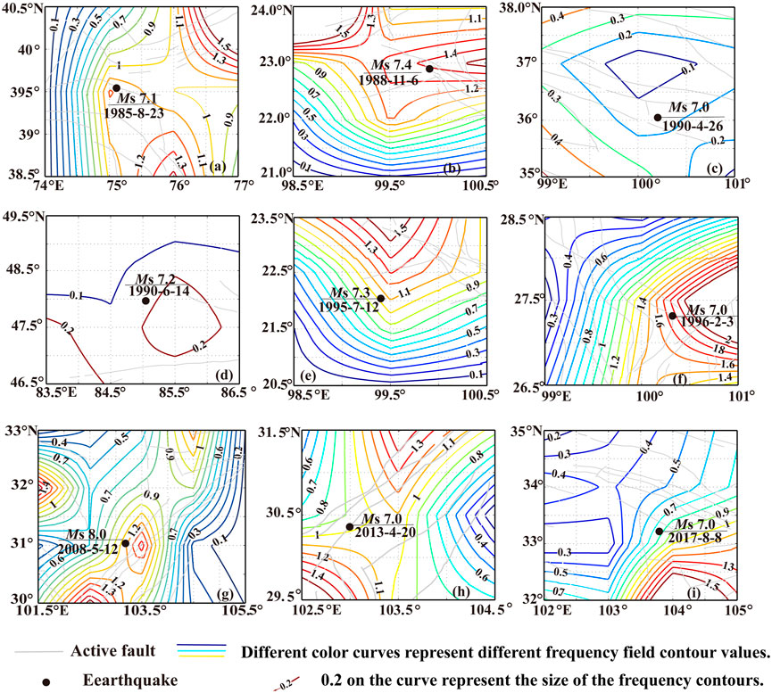
FIGURE 4. Frequency field contour maps of 9 Ms ≥7.0 earthquakes that occurred in mainland China, the black dots represent earthquakes, the blue, green, orange and red lines represent frequency field contours, and the gray lines represent active faults. (A) 1985 Ms 7.1 Wuxia earthquake; (B) 1988 Ms 7.6 Lancang–Gengma earthquake; (C) 1990 Ms 7.0 Gonghe earthquake; (D) 1990 Ms 7.2 Jeminay earthquake; (E) 1995 Ms 7.3 Myanmar–China earthquake; (F) 1996 Ms 7.0 Lijiang earthquake; (G) 2008 Ms 8.0 Wenchuan earthquake; (H) 2013 Ms 7.0 Lushan earthquake; (I) 2017 Ms 7.0 Jiuzhaigou earthquake.

It may be possible to preliminarily locate the epicenter of future Ms ≥7.0 earthquakes in a study area by studying the variations of its frequency-field contours. The January 1998–April 2008 frequency-field contour map of the 2008 Ms 8.0 Wenchuan Earthquake (Table 1; Figure 4G) exhibits three vortex-like isocratic anomalies (areas with high densities of contours with values greater than 0.9). The anomalies centered around (31.0°N, 103.5°E) and (30.0°N, 102.5°E) correspond to the epicenters of the 2008 Ms 8.0 Wenchuan Earthquake and 2013 Ms 7.0 Lushan Earthquake, respectively, whereas the anomaly centered around (31.5°N, 101.5°E) might be related to the 2014 Ms 6.3 Kangding Earthquake. The strong earthquakes that occurred persistently around the Longmenshan Fault after 2009 might have been triggered by the frequency field anomalies of the 2008 Ms 8.0 Wenchuan Earthquake. For brevity, we will simply describe the pre-quake frequency-field contour anomalies associated with the eight other Ms ≥7.0 earthquakes in Table 1 instead of providing a detailed analysis of each earthquake.

3 Discussion

3.1 Comparison between regional earthquake frequency graphs and earthquake frequency fields

Several scholars (Feng et al., 2009; Li et al., 2017; Zhang and Li, 2021) took the area around the epicenter of a strong earthquake as the research area to study the frequency anomaly of regional seismic activity before a strong earthquake. In this paper, the natural orthogonal expansion method is mainly used to study the typical frequency field in the strong earthquake area. The regional earthquake frequency graphs of 9 Ms ≥7.0 earthquakes (with 3-month frequencies) were compared with their T₁–T₄ graphs; the use of frequency graphs is a conventional seismological method, whereas the use of T₁–T₄ graphs is the method proposed in this paper. Owing to length constraints, this comparison was limited to the 1995 Ms 7.3 Myanmar–China Earthquake and the 2008 Ms 8.0 Wenchuan Earthquake. The earthquake frequency graph of the 1995 Ms 7.3 Myanmar–China Earthquake strongly resembles its T₁ graph (Figure 5 top). Based on Tables 1, 2, the accuracy of T₁–T₄ for this earthquake is 99.34% and the fit of T₁, which is the primary field of the frequency field, is 48.6%. Therefore, the earthquake frequency graph is simply a part of T₁–T₄ and the information carried by the former is contained within the latter. The earthquake frequency graph of the 2008 Ms 8.0 Wenchuan Earthquake also closely resembles the T₁ graph, which is the primary field of the frequency field (Figure 5 bottom); the information within the earthquake frequency graph is effectively contained in the T₁ graph. The same relation was observed for all other Ms ≥7.0 earthquakes.

FIGURE 5

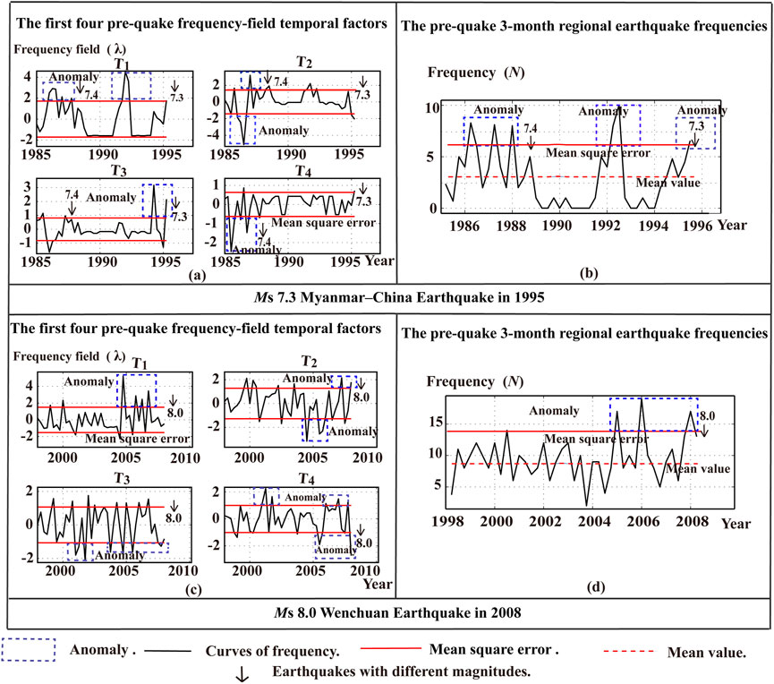
FIGURE 5. Comparison between frequency-field temporal factors and regional earthquake frequency graphs, the green dotted line represents the anomaly, the red line is two times the mean square error, the black arrow represents the magnitude of a Ms ≥7.0 earthquake, the red dotted line is the mean line (A,B)the 1995 Ms 7.3 Myanmar–China earthquake (top), (C,D) the 2008 Ms 8.0 Wenchuan earthquake (bottom).

Table 1 shows a partial overlap between the study areas of the 1995 Ms 7.3 Myanmar–China Earthquake (20.0°N–23.0°N, 98.5°E–100.5°E) and 1988 Ms 7.4 Lancang–Gengma Earthquake (21.5°N–23.5°N, 99.0°E–101.0°E). It is seen that the temporal spans of these earthquakes also overlap, with temporal spans of January 1985—June 1995 and January 1975—October 1988, respectively. As a result, both Figures 5A, B exhibit medium and short-term pre-quake anomalies prior to the earthquake and high-value anomalies that always correspond to strong earthquakes. The T₂, T₃, and T₄ graphs in Figure 5A also contain the short-term and imminent anomalies of the 1995 Ms 7.3 Myanmar–China earthquake and are more accurate than the regional earthquake frequency graph. This result highlights the advantage of using natural orthogonal expansion to study earthquake frequency fields.

3.2 Comparison between cumulative earthquake frequency graphs and earthquake frequency fields

The seismic activities that occur in the study area of an Ms ≥7.0 earthquake include its background seismicity, which comprises small random quakes, and strong earthquake precursors that manifest as small anomalous quakes. These seismic activities are controlled by different stress mechanisms. Background seismicity is controlled by stable long-term and region-wide stresses and is a relatively stable process. The cumulative earthquake frequency owing to background seismicity generally increases linearly over time, with small fluctuations, and it represents the equilibrium state of the region. By contrast, small anomalous quakes are caused by localized short-range stresses in the vicinity of seismic sources or fault junctions. They typically occur in highly seismic-sensitive regions; once their mechanical equilibrium is disrupted, the cumulative earthquake frequency will decrease or increase significantly over time owing to tectonic stress, thus causing the cumulative earthquake frequency graph to become non-linear (Figure 6).

FIGURE 6

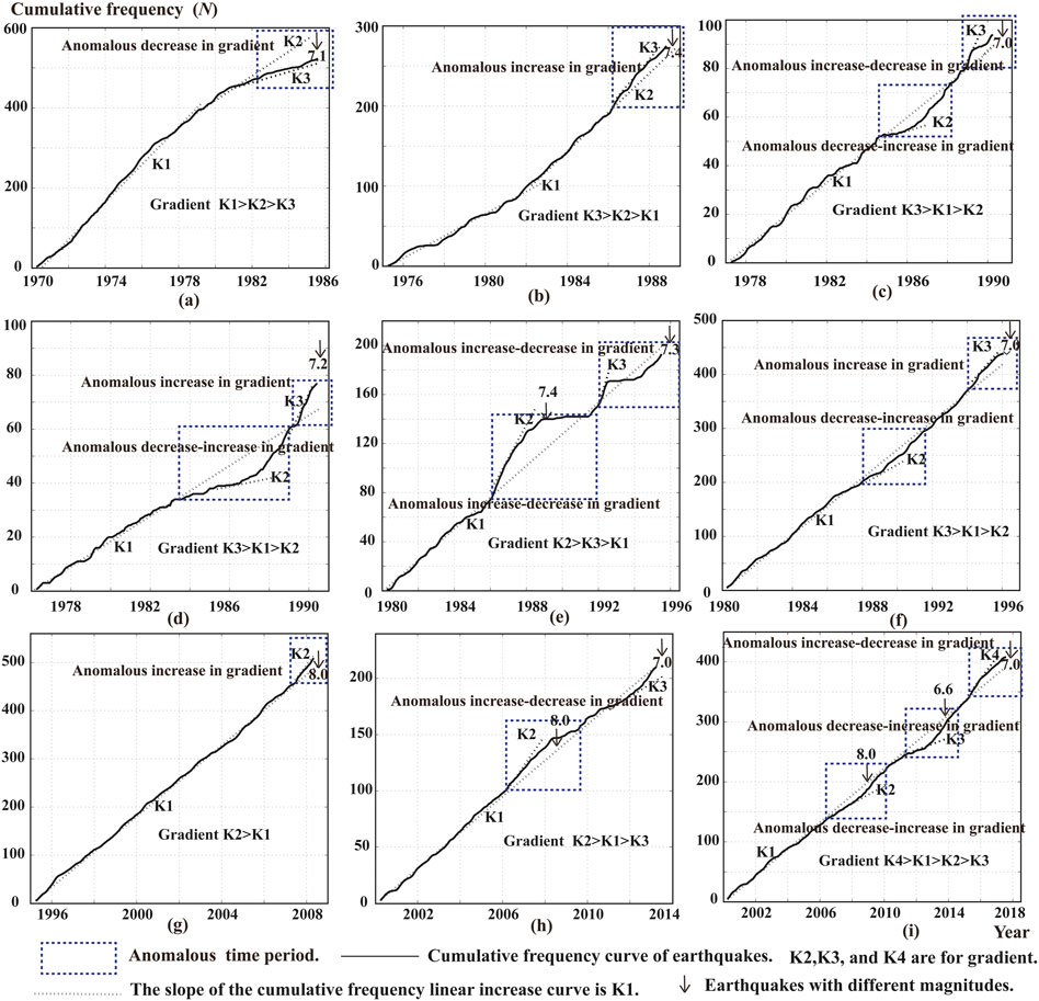
FIGURE 6. Cumulative frequency graphs of 9 Ms ≥7.0 earthquakes, the green dotted line represents the anomaly, the black arrow represents the magnitude of a Ms ≥7.0 earthquake, the dashed line represents the slope of a linear increase in cumulative frequency, K1, K2, K3, and K4 are for gradient. (A) 1985 Ms 7.1 Wuxia earthquake; (B) 1988 Ms 7.6 Lancang–Gengma earthquake; (C) 1990 Ms 7.0 Gonghe earthquake; (D) 1990 Ms 7.2 Jeminay earthquake; (E) 1995 Ms 7.3 Myanmar–China earthquake; (F) 1996 Ms 7.0 Lijiang earthquake; (G) 2008 Ms 8.0 Wenchuan earthquake; (H) 2013 Ms 7.0 Lushan earthquake; (I) 2017 Ms 7.0 Jiuzhaigou earthquake.

Application of earthquake cumulative frequency method (Ma et al., 2008; Ma et al., 2022) The study of the non-linear variation law of regional seismic activity before strong earthquakes can better explain the seismic frequency field anomalies in this paper. The pre-quake cumulative earthquake frequency graphs of the 9 Ms ≥7.0 earthquakes are shown in Figure 6. In the normal state, the cumulative earthquake frequency graph will extend linearly over time. If a significant decrease or increase in seismic activity occurs, the gradient of the graph will decrease or increase significantly, which is indicative of seismic locking around the seismic source zone or fault as well as enhanced seismic activity. In the pre-quake cumulative earthquake frequency graph of the 2017 Ms 7.0 Jiuzhaigou Earthquake (Table 3), it is seen that the graph is linear from January 2000—July 2006 with a gradient of K1. The gradient of the graph decreases significantly (to K2) from August 2006, indicating an abnormal seismic state. This is quickly followed by the medium-to-imminent anomalies of the 2008 Ms 8.0 Wenchuan Earthquake, after which the graph returns to its equilibrium state (K1). The cumulative earthquake frequency graph decreases to K3 in October 2011 and then exhibits the medium-to-short term anomalies of the 2013 Ms 6.6 Gansu Earthquake before returning to the equilibrium state. In June 2015, the gradient of the cumulative earthquake frequency graph rises to K4, where it remains until the 2017 Ms 7.0 Jiuzhaigou Earthquake; this increase in gradient is the medium-to-short term anomaly that precedes the 2017 Ms 7.0 Jiuzhaigou Earthquake. Long-term or medium-to-imminent anomalies in the pre-quake cumulative earthquake frequency graph always precede the occurrence of a strong earthquake in all other Ms ≥7.0 earthquakes (Table 3).

TABLE 3

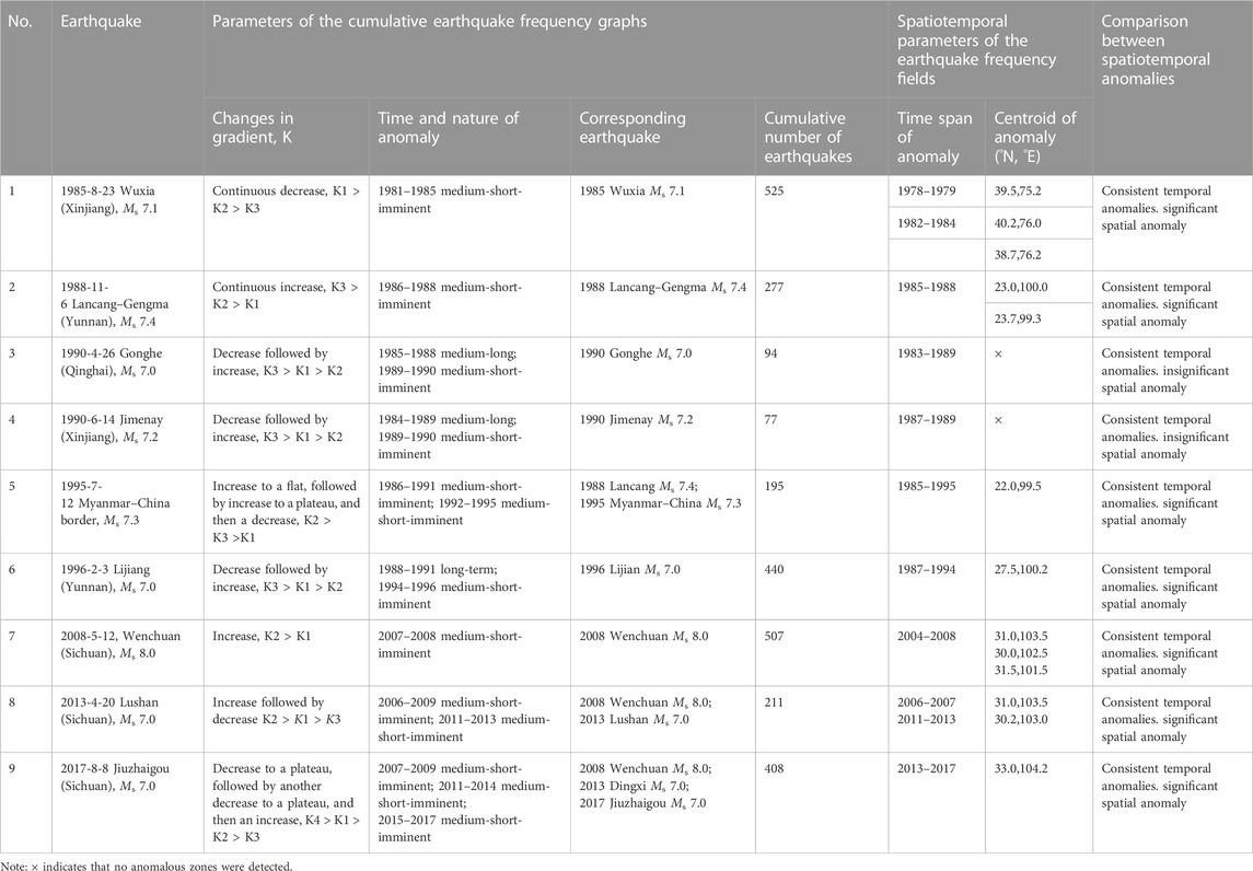
TABLE 3. Comparison between the cumulative earthquake frequency graphs and frequency field anomalies of 9 M_s ≥7.0 earthquakes in China.

The timing and nature of the anomalies in the cumulative earthquake frequency graphs are listed in Table 3. The nature of each anomaly was determined with respect to its corresponding earthquake and the cumulative earthquake frequency graphs were calculated using the same number of samples as were used to create the contours in Figure 4. It is seen from the table that the spatial anomalies of the frequency-field contours appear to be insignificant if an insufficient number of samples are available. In each study area, the temporal anomalies of the cumulative earthquake frequency graph and frequency field generally agree in terms of time span. By comparing the cumulative earthquake frequency graphs and frequency fields of the 9 Ms ≥7.0 earthquakes, we found that the frequency-field temporal anomalies and spatial contours calculated via natural orthogonal expansion are highly accurate and reliable. This result is consistent with the spatiotemporal anomaly of the magnitude frequency distribution inferred by Ogata and Katsuta (1993).

3.3 Comparison between strain fields and frequency fields

The seismic strain field method (Yang et al., 2017; Luo et al., 2018; Lu et al., 2019a) is the same as the frequency field method, except that the parameter variables are different. The seismic strain field takes the seismic strain as the independent variable, and the frequency field takes the frequency as the independent variable. A comparison between the frequency and strain fields of the 1995 Ms 7.3 Myanmar–China Earthquake and the 2008 Ms 8.0 Wenchuan Earthquake is shown in Figure 7. It is seen that the frequency-field temporal factors are highly sensitive to seismic anomalies, as they exhibit large fluctuations and complex anomaly patterns. Conversely, the strain-field temporal factors are largely noiseless and exhibit clear and distinct pre-quake anomalies. However, the frequency-field temporal factors can reflect the anomaly patterns of multiple Ms ≥7.0 earthquakes if they have overlapping study areas (Figure 7A). Conversely, the strain field can only reflect pre-quake anomalies associated with large accumulations (or releases) of strain energy, as smaller anomalies are masked in the strain-field temporal factors (Figure 7B). The results are consistent with the cumulative growth anomaly results of non-linear earthquakes Ma et al. (2022).

FIGURE 7

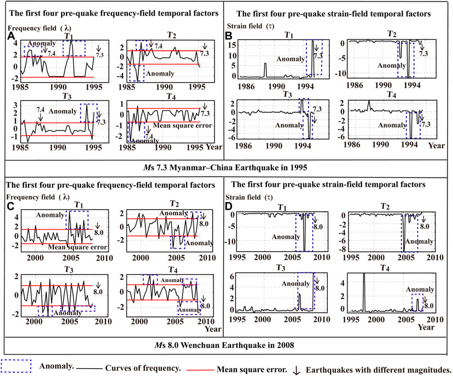
FIGURE 7. Comparison between frequency-field and strain-field temporal factors, the green dotted line represents the anomaly, the red line is two times the mean square error, the black arrow represents the magnitude of a Ms ≥7.0 earthquake (A,B) the 1995 Ms 7.3 Myanmar–China earthquake (top) and (C,D)the 2008 Ms 8.0 Wenchuan earthquake (bottom).

3.4 Discussion on the rationality of the selection of time interval and space scale

In the selection of seismic spatial scale, the seismicity statistical area related to large earthquakes and the grid cell are determined separately. Mei (1997) studied an Ms ≥7.0 earthquake in the North China Plain and found that its seismic activity occurred in three stages: an initial low level, a gradually increasing phase, and a final weakening phase. The statistical area over which the earthquake occurred changed over time from 500 to 400 km; as seismic activity developed, the area was gradually reduced. Further measurements taken from 20 Ms 6.0–6.9 earthquakes occurring in China revealed pre-earthquake activity enhancement areas ranging from 180 to 390 km. Based on these data, we applied a natural orthogonal function expansion to select a range of 3° in both longitude and latitude around the epicenter as the study area. The grid cells calculated using this approach reflected the distribution characteristics of regional seismic frequency but were too densely clustered. If 0.5°×0.5°grid cells were used, the frequency field curves would be averaged and the abnormal characteristics of the main frequency fields would not be effectively highlighted. If instead a 1.5°×1.5°grid cell was selected, the grid could be too large and the primary anomaly would be concentrated in the first frequency field in a manner similar to the results for the overall study area (Figure 4B), losing the multi-component characteristics of the results. In our paper, we reference Ma et al. (2020) discussion of these specific factors; we directly cite their research results and optimize the grid cell to 1.0°×1.0°.

The time interval is taken as a sliding calculation over 3 months because an interval of two or 4 months would have a negative influence on the sliding calculation results. If the time interval were too short, there would be more data, making anomalies more prominent, but the calculation speed would be slow. Increasing the time interval would speed up the computation but reduce the amount of data, masking anomalies. Thus, we followed the detailed discussion by Ma et al. (2020) and set a sliding of window of 3 months to obtain the best calculation results.

4 Conclusion

In this study, we analyzed the anomalies in the frequency-field temporal factors and spatial contours that preceded 9 Ms ≥7.0 earthquakes in mainland China. The following conclusions were drawn from the results of this analysis:

Prior to an Ms ≥7.0 earthquake, three to four of the first four frequency fields always exhibit anomalous changes in their temporal factors. The vast majority of these temporal anomalies are concentrated in the first four frequency fields and the anomalies appear to comprise multiple components. The contribution of T₁ to these anomalies is the largest among all temporal factors (typically 40%–60%) and the T₁ graph strongly resembles the regional (3-month) earthquake frequency graph. The proposed natural orthogonal expansion-based frequency field approach is more accurate than the conventional method and can be used to detect short-term and imminent seismic anomalies.

Frequency-field temporal factors are highly sensitive to seismic anomalies, as their graphs exhibit large fluctuations and complex anomaly patterns (rising, falling, fluctuating, rising and then falling, falling and then rising, etc.). This is because the frequency-field temporal factors depend only on the number of small earthquakes within a region. For instance, the contribution of an M_L 2.7 earthquake to the frequency field is identical to that of an M_L 5.3 earthquake. The strain field (seismic energy field) graph is much more “noiseless,” which results in highly distinct anomaly peaks. This is because the strain field depends on the cumulative seismic strain (or energy) of the quake; a difference of one in magnitude corresponds to a 33-times difference in strain (energy). Therefore, the contribution of an M_L 2.7 quake to a strain field graph is much smaller than that of an M_L 5.3 quake, and the signals of smaller strains are often masked by those of larger strains. The frequency field is more adept than the strain field at highlighting the pre-quake temporal anomalies of different Ms ≥7.0 earthquakes if there is some overlap in their affected areas, as these anomalies are usually masked in strain fields.

High-gradient turning points are present in the spatial contours of pre-quake frequency fields of Ms ≥7.0 earthquakes. Areas that have high densities of contour lines and contour values greater than 0.9 (where the blue lines change into red lines in Figure 4) are high-risk zones for strong earthquakes as they have the potential to generate large events. The detection of danger zones using frequency-field spatial contours is strongly dependent on the number of earthquake samples in the dataset; generally, increasing the number of earthquakes increases the reliability of forming contour danger zone.

If the seismic stresses of a region are in a normative state, the cumulative earthquake frequency curve of the region should increase linearly over time and its seismic events should be normally distributed. An anomalous increase or decrease in the gradient of the cumulative earthquake frequency graph is indicative of a significant calming of or increase in the seismic activity around a seismic source zone or fault junction. The anomalies of the cumulative earthquake frequency graph and frequency-field temporal factors are generally consistent with each other in terms of their time spans. Therefore, the temporal factor anomalies that are computed using the proposed method are reliable.

The natural orthogonal expansion calculation method proposed in this study is novel and abandons the use of the conventional earthquake region as the research object. In the proposed approach, the natural frequency orthogonal field expansion method is used to calculate the typical frequency fields related to larger earthquakes occurring in an area, from which points can be extracted from the characteristics of short and intermediate anomalies in primary seismic frequency that precede earthquakes with magnitudes greater than 7. This provides a reference for the prediction of large earthquakes occurring on the Chinese mainland. This study had the following limitations: the time factor used to describe the typical frequency field is sensitive; in addition, the curves generated using the proposed approach fluctuate significantly and have an abnormal shape that is complex and difficult to identify.

Data availability statement

The original contributions presented in the study are included in the article/supplementary material, further inquiries can be directed to the corresponding author.

Author contributions

All authors contributed to the conception and design of this study. GL, FD, and MY prepared the material, collected the data, and performed the analysis. The first draft of the manuscript was written by GL, and all authors provided their feedback on previous versions of the manuscript. All authors have read and approved the final manuscript. Sincerely, GL, FD, HM, MY Seismological Bureau of NH Autonomous Region.

Funding

This work was supported by the Earthquake Science and Technology Spark Plan Project (XH18052) and the Ningxia Natural Science Foundation Project (2021AAC03483).

Acknowledgments

We are very thankful for the guidance and help of Puqiong Huang of the seismic network center of China Seismological Bureau. Thanks to the reviewers for their valuable revision suggestions, and especially thanks to the responsible editors for their patient answers and help.

Conflict of interest

The authors declare that the research was conducted in the absence of any commercial or financial relationships that could be construed as a potential conflict of interest.

Publisher’s note

All claims expressed in this article are solely those of the authors and do not necessarily represent those of their affiliated organizations, or those of the publisher, the editors and the reviewers. Any product that may be evaluated in this article, or claim that may be made by its manufacturer, is not guaranteed or endorsed by the publisher.

References

Aden-Antóniow, F., Satriano, C., Bernard, P., Poiata, N., Aissaoui, E.-M., Vilotte, J.-P., et al. (2020). Statistical analysis of the preparatory phase of the M_W 8.1 Iquique earthquake, Chile. JGR Solid Earth 125, e2019JB019227. doi:10.1029/2019JB019337

CrossRef Full Text | Google Scholar

Feng, J. G., Zhou, L. Q., Yang, L. M., and Dai, W. (2009). Anomaly of small earthquake activities before medium to strong earthquakes in the northeast margin of the Qinhai-Tibe block. Earthq. (in Chin. 29 (3), 19–26.

Google Scholar

Jarmolowski, W., Belehaki, A., Hernandez, P. M., Schmidt, M., Goss, A., Wielgosz, P., et al. (2021). Combining swarm Langmuir probe observations, LEO-POD-based and ground-based GNSS receivers and ionosondes for prompt detection of ionospheric earthquake and tsunami signatures: Case study of 2015 Chile-Illapel event. J. Space Weather Space Clim. 11, 58. doi:10.1051/SWSC/2021042

CrossRef Full Text | Google Scholar

Katsumata, K. (2011). A long-term seismic quiescence started 23 years before the 2011 off the Pacific coast of Tohoku earthquake (M=9.0). Earth Planets Space 63, 709–712. doi:10.5047/eps.2011.06.033

CrossRef Full Text | Google Scholar

Li, Y. E., Chen, L. J., and Chen, X. Z. (2017). Enhancement of seismicity recorded by the Qiaojia seismic network before the 2013 Lushan and 2014 Ludian earthquakes. Earthq. (in Chin. 37 (3), 95–105.

Google Scholar

Luo, G. F., Liu, Z. W., Ding, F. H., Ma, H. Q., and Yang, M. Z. (2018). Research on the seismic strain field prior to the 2017 Jiuzhaigou, Sichuan Ms7.0 earthquake. China Earthq. Eng. J. 40 (6), 1322–1330. doi:10.3969/j.issn.1000-0844.2018.06.1322

CrossRef Full Text | Google Scholar

Luo, G. F., Liu, Z. W., Luo, H. Z., and Ding, F. H. (2019b). Effect of the strain field of Wenchuan 8 earthquake on the strong earthquake around the epicenter. Prog. Geophys. (in Chinese) 34 (3), 908–918. doi:10.6038/pq.2019CC0454

CrossRef Full Text | Google Scholar

Luo, G. F., Tu, H. W., and Ding, F. H. (2019a). Spatio-temporal anomaly characteristics of regional seismic strain field before large earthquakes. Earthquake (in Chinese) 39 (2), 63–76.

Google Scholar

Luo, G. F., Tu, H. W., Ma, H. Q., and Yang, M. Z. (2011b). Analysis on energy field of the seismic activity in earthquake hazard area from the northwest to the south of Yunnan. Journal of Seismological Research (in Chinese) 34 (4), 285–291.

Google Scholar

Luo, G. F., Yang, M. Z., Ma, H. Q., and Xu, X. Q. (2011a). Intermediate and short-term anomalies of seismic activity energy field before the Wenchuan Ms 8.0 earthquake. Earthquake (in Chinese) 31 (3), 135–142.

Google Scholar

Luo, G. F., and Yang, M. Z. (2005). Space-time distributed characteristics on energy field of earthquake in the Yunnan region. Earthquake Research in China 21 (3), 13–18.

Google Scholar

Luo, G. F., Zeng, X. W., Ma, H. Q., and Yang, M. Z. (2014). Analysis of energy field of seismic activity before the minxian-zhangxian Ms6.6 earthquake in China. Earthquake Engineering Journal (in Chinese) 36 (2), 314–319. doi:10.3969/j.issn.1000-0844.2014.02.0314

CrossRef Full Text | Google Scholar

Ma, H. Q., Yang, M. Z., Ding, F. H., and Luo, G. F. (2022). Nonlinear analysis on seismic activity before Ms ≥7.0 earthquakes occurred in Chinese mainland. Earthquake Research in China 38 (1), 42–51.

Google Scholar

Ma, H. Q., Yang, M. Z., and Li, C. G. (2008). The theory explanation and application examples concerning the changes of small earthquake occurrence rate and accumulation time. Earthquake (in Chinese) 28 (1), 57–64.

Google Scholar

Ma, H. Q., Yang, M. Z., and Luo, G. F. (2020). Study on frequency field of seismic activity. Earthquake (in Chinese) 40 (3), 99–111. doi:10.12196/j.issn.1000-3274.2020.03.008

CrossRef Full Text | Google Scholar

Ma, H. Q., and Yang, M. Z. (2012). Research on the energy field about Yushu ms 7.1 earthquake in Qinghai in 2010. Journal of Seismological Research (in Chinese) 35 (4), 487–490.

Google Scholar

Ma, K. Y., Ding, Y. G., and Tu, Q. (1993). Principles and methods of climate statistics. China: Beijing Press Meteorological.

Google Scholar

Mei, S. R. (1997). General characteristics of long term evolution of seismicity before strong earthquakes in North China//Theory and method of short impending earthquake prediction. China: Beijing Press Seismological.

Google Scholar

Mei, S. R. (1996). On the physical model of earthquake precursor fields and the mechanism of precursors’ time-space distribution (III) — Anomalies of seismicity and crustal deformation and their mechanisms when a strong earthquake is in preparation. Acta Seismologica Sinica 9 (2), 223–234. doi:10.1007/bf02651066

CrossRef Full Text | Google Scholar

Mogi, K. (1969). Some features of recent seismic activity in and near Japan (2) : Activity before and after great earthquakes. Bull. Earthquake. Res. Inst. Univ. Tokyo 47, 395–417.

Google Scholar

Ogata, Y., and Katsuta, K. (1993). Analysis of temporal and spatial heterogeneity of magnitude frequency distribution inferred from earthquake catalogues. Geophysical Journal International 113 (3), 727–738. doi:10.1111/j.1365-246x.1993.tb04663.x

CrossRef Full Text | Google Scholar

Wang, Y. W., Jiang, C. S., Liu, F., and Bi, J. M. (2017). Assessment of earthquake monitoring capability and score of seismic station detection capability in China Seismic Network (2008-2015). Chinese J. Geophys (in Chinese) 60 (7), 2767–2778. doi:10.6038/cjg20170722

CrossRef Full Text | Google Scholar

Wiemer, S., and Wyss, M. (1994). Seismic quiescence before the Landers (M=7.3) and big bear (M=6.5) 1992 earthquakes. Bull. Seismic. Soc. Am. 84, 900–916.

Google Scholar

Wyss, M., and Habermann, R. E. (1998). Precursory seismic quiescence. Pageoph 126 (2), 319–332. doi:10.1007/bf00879001

CrossRef Full Text | Google Scholar

Yang, M. Z., and Ma, H. Q. (2013). Features of time factor anomalies of regional energy field before large earthquake. Earthquake (in Chinese) 33 (3), 107–115.

Google Scholar

Yang, M. Z., and Ma, H. Q. (2012). Analysis of regional seismic energy field before Wenchuan Ms 8.0 earthquake. Progress in Geophysics (in Chinese) 27 (3), 0872–0877. doi:10.6038/j.issn.1004-2903.2012.03.006

CrossRef Full Text | Google Scholar

Yang, M. Z., Ma, H. Q., Luo, G. F., and Xu, X. Q. (2017). Research on the seismic strain field before strong earthquakes above Ms6 in Chinese mainland. Chinese Journal of Geophysics 60 (10), 3804–3814. doi:10.6038/cjg20171010

CrossRef Full Text | Google Scholar

Yang, M. Z., and Ma, H. Q. (2004). Statistical analysis of seismic activity energy field in Ningxia and its adjacent areas. Journal of Earthquake (in Chinese) 26 (5), 516–522.

Google Scholar

Yang, M. Z., and Ma, H. Q. (2011). Variation of energy field of Longmenshan fault zone before the Wenchuan M_S 8.0 earthquake. Earthquake Research in China 27 (3), 260–267.

Google Scholar

Zhang, B., and Li, M. J. (2021). Characteristics of seismicity anomalies before the 2021 Ms 7.4 earthquake in Qinghai Province. China Earthquake Engineering Journal (in Chinese) 43 (4), 826–833. doi:10.3969/j.issn.1000-0844.2021.04.826

CrossRef Full Text | Google Scholar