Physical–empirical prediction model for the dominant mode of extreme high temperature events in eastern China during summer

The dominant mode of extreme high temperature events in eastern China during summer shows a dipole pattern with opposite anomalies over southern and northeastern China, which explains 25% of the variance. We document the limited prediction skill of the National Centers for Environmental Prediction Climate Forecast System, version 2 (CFSv2) for the dominant mode of these events. Based on the mechanisms related to the dominant mode, a physical–empirical model was established that improved the prediction of extreme high temperature events in eastern China, which will help in disaster prediction and mitigation. The physical connection between the dominant mode and the summer sea surface temperature (SST) over the western tropical and subtropical Pacific Ocean was predicted well by the CFSv2 hindcasts, and thus the areal mean CFSv2-hindcast SSTs over the western tropical and subtropical Pacific Ocean served as a predictor in the physical–empirical model. In the observations, the soil moisture over southern China in the preceding December (soil_Dec) combined the signal of the air–sea interactions over the tropical and northern extratropical Pacific Ocean, which induced anomalous SSTs in the Indian and western tropical Pacific oceans in the following summer and contributed to the dominant mode. Soil_Dec was therefore closely correlated with the dominant mode and was used as a predictor. The results of the one-year-leave cross-validation and independent hindcast showed that the time series of the dominant mode was better predicted by the physical–empirical model than by the CFSv2 hindcasts, with an improved correlation coefficient from insignificant to about 0.8, a root-mean-square error reduced by about 50% and an increased rate of same signs. The physical–empirical model showed advantages in the prediction of the dominant mode of summer extreme high temperature events over eastern China, which may be used in the prediction of other climate variables.

Introduction

Extreme high temperature events (EHEs) are occurring with increasing frequency as a result of the global climate crisis, exerting a greater influence on human health, the social economy and the ecological environment (Chen et al., 2019; Borg et al., 2021; Igun et al., 2022). The number of deaths related to EHEs increased markedly in the decade from 2000 to 2010 compared with the decade from 1991 to 2000, accounting for a large proportion of the increased deaths caused by extreme climate events such as floods and droughts (WMO 2013). Model simulations indicate that EHEs will occur more frequently and with greater intensity in the future (Orlowsky and Seneviratne 2012; Chen and Sun 2018). It is therefore important for disaster prevention and reduction to investigate the variations in EHEs, to understand the associated mechanisms and to improve their prediction.

Eastern China is vulnerable to EHEs, which show a large variability in this region (Sun et al., 2014; Deng et al., 2019). Previous studies have shown that the frequency of EHEs (FEHEs) over China is characterized by variability on different timescales (You et al., 2017; Chen et al., 2018; Zhu et al., 2020b). You et al. (2017) showed that the FEHEs based on relative and absolute definitions has increased over the whole of China, particularly after 1990, reflecting rapid warming after this time. Superimposed on these long-term trends, there are also dominant interdecadal and interannual spatiotemporal variations in FEHEs over eastern China (Zhu et al., 2020b; Hong et al., 2020; Liu et al., 2021; Yang et al., 2021; Zhu et al., 2022). The interannual variability of FEHEs is relatively large over eastern China, which greatly contributes to the overall variability (Chen et al., 2018; Deng et al., 2019).

The prediction skill of current dynamic models for extreme climate events is limited (Pepler et al., 2015; Gao et al., 2018; Luo et al., 2020; Tang et al., 2021a; Tang et al., 2021b) and physical–empirical models have been used to improve predictions (Ji and Fan 2019; Yang et al., 2019; Tian and Fan 2020; Long et al., 2022). The crucial procedure in physical–empirical models is the detection of physically meaningful predictors (Gao et al., 2018; Han et al., 2020; Long et al., 2022). A combination of predictors from dynamic prediction systems and predictors in the observations includes the dynamic processes revealed in the dynamic models and the observations, improving the prediction skill (Zhang et al., 2019a; Zhang et al., 2019b; Chen and Sun 2020).

We need a better understanding of the mechanisms related to predictands to establish physical–empirical models. Many studies have analyzed the anomalous atmospheric circulation responsible for the occurrence of EHEs over China and the influence from the tropics and mid to high latitudes (Deng et al., 2019; Xu et al., 2019; Zhu et al., 2020a; Long et al., 2022; Zhou et al., 2022). The anomalous intensity or location of the western Pacific subtropical high could induce anomalous vertical motion and transport of water vapor over China, leading to anomalous adiabatic heating and surface heat fluxes, which could contribute to the occurrence of EHEs over China (Li et al., 2020; Ren et al., 2020). Several factors, such as the El Niño–Southern Oscillation (ENSO) and the sea surface temperature (SST) in the Indian Ocean, account for the variations in the western Pacific subtropical high (Zhang et al., 2019c; Sun et al., 2019; Tong et al., 2020) and could be considered as potential predictors for the FEHEs over eastern China. In addition, the mid- and high-latitude wave train propagating eastward to East Asia could also induce anomalous atmospheric circulation and contribute to the variations in the FEHEs over China, which may be associated with air–sea interactions over the North Atlantic, sea ice in the Arctic region and other factors (Li et al., 2018; Zhu et al., 2020a, 2022).

Most studies have focused on the simultaneous atmospheric circulation anomalies and influential factors related to EHEs. We therefore aimed to investigate the following two questions: 1) how are the dominant mode of the interannual variability of summer FEHEs over eastern China, the associated atmospheric circulation and SST anomalies predicted in the dynamic model; and 2) could a physical–empirical model be established to improve the prediction of the dominant mode of FEHEs over eastern China?

The rest of the paper is organized as follows. Section 2 introduces the data and methods. Section 3 investigates the prediction ability of the National Centers for Environmental Prediction (NCEP) Climate Forecast System, version 2 (CFSv2) for the dominant mode of the FEHEs over eastern China during summer. The predictors used in the physical–empirical model are detected and their physical connection to the dominant mode of the FEHEs are analyzed in Section 4. Section 5 presents the establishment and estimation of the physical–empirical model and conclusions are presented in Section 6.

Data and methods

Data

We calculated the FEHEs using the daily observed maximum temperature during summer (June−July−August) from the CN05.1 dataset, a gridded observational dataset with a resolution of (0.25°×0.25°) based on data from observational stations in China (Wu and Gao 2013). We obtained the monthly mean 850 hPa horizontal wind, 500 hPa vertical velocity with a resolution of (2.5°×2.5°) and surface net shortwave radiation with a resolution of 92×192 grid points from the NCEP (Kalnay et al., 1996). We also used the Extended Reconstructed SST V5 with a resolution of (2°×2°) (Huang et al., 2017) and Climate Prediction Center (CPC) soil moisture with a resolution of 360×720 grid points (Huang et al., 1996) from the National Oceanic and Atmospheric Administration.

The hindcasts of the daily maximum temperature and monthly SSTs in summer were derived from the CFSv2, which is a state-of-the-art prediction system with interactions between the ocean, atmosphere and land on a global scale (Saha et al., 2014). The CFSv2 hindcasts were integrated for 9 months, with initial conditions every 5 days from 11 April to 6 Ma y, and we used the ensemble mean of the forecasts for summer. The CFSv2 data with a resolution of (1°×1°) cover the time period 1982–2018 and we selected the other observational and reanalysis data to be consistent with this time period. Both the observational and reanalysis data are referred to as observations to distinguish them from the prediction data in the CFSv2 hindcasts.

Methods

Taking into consideration the different climate states in different regions of China, we adopted the relative definition of EHEs—that is, we used the 95% percentile value of the daily maximum temperature during summer as the threshold (Zhu et al., 2020a; Long et al., 2022; Zhu et al., 2022). The threshold was different between grids and the number of days with maximum temperatures exceeding the threshold during summer was defined as the FEHEs. Because this study focused on the interannual variability, we applied Fourier analysis to all data before other calculations such as empirical orthogonal function decomposition, correlation analysis and so on, and the 9-year high-pass variability was reserved (Bloomfield 2004).

The linear signal of one variable (X) is removed from the other variable (Y) based on the following formula (Sun et al., 2019):

${\mathrm{Y}}^{*}=\mathrm{Y}–\mathrm{X}\times \mathrm{c}\mathrm{o}\mathrm{v}\left(\mathrm{X},\mathrm{Y}\right)/\mathrm{v}\mathrm{a}\mathrm{r}\left(\mathrm{X}\right),$

where X and Y are the original time series, $\mathrm{c}\mathrm{o}\mathrm{v}\left(\mathrm{X},\mathrm{Y}\right)$ represents the temporal covariance between X and Y, $\mathrm{v}\mathrm{a}\mathrm{r}\left(\mathrm{X}\right)$ represents the variance of X, and ${\mathrm{Y}}^{*}$ represents the time series of Y with the linear signal of X removed.

We used the one-year-leave cross-validation and independent hindcast methods to estimate the prediction of the physical–empirical model. We used one-year-level cross-validation to predict the predictand in the specific year using the remaining years as the training period to build the physical–empirical model. The independent hindcast was similar to the real prediction and we chose the first training period—for example, the data for 1982–1999 were used to establish the first physical–empirical model and give the prediction in 2000 and then the data for 1982–2000 were used to build the second physical–empirical model and make the prediction in 2001, and so on. We used the prediction for 2000–2018 for verification. The prediction skill of the physical–empirical model was mainly reflected through the correlation coefficient, the root-mean-square error (RMSE) and the rate of same signs. The significance test of the correlation coefficient was based on Student’s t-test.

Prediction skill of the CFSv2 hindcasts for the dominant mode of the FEHEs

To understand the skill of the CFSv2 hindcast data in predicting the FEHEs over eastern China, we analyzed the characteristics of FEHEs in the CFSv2 hindcasts and the observations. Figure 1A shows the standard deviation of FEHEs over eastern China in the observations, with two centers of relatively large values over southern and northeastern China. The center of relatively large standard deviations over northeastern China was captured in the CFSv2 hindcasts (Figure 1B), but the standard deviation was overestimated over northeastern and central China and underestimated over southern China (Figure 1A,B). Figure 1C shows that the RMSE between the FEHEs in the observations and the CFSv2 hindcasts was almost greater than one standard deviation over eastern China, with relatively large values over central China. The time correlation coefficients between the observed FEHEs and the CFSv2 hindcast FEHEs showed scattering positive correlation over northern and southern China (Figure 1D). The spatial discrepancies in the standard deviation (Figure 1A,B), the relatively large RMSE (Figure 1C) and the low time correlation coefficients (Figure 1D) indicate the limited prediction skill of the CFSv2 hindcasts for the FEHEs over eastern China.

FIGURE 1

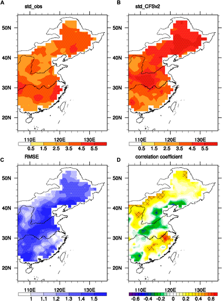
FIGURE 1. Standard deviation of FEHEs over eastern China during summer in (A) the observations and (B) the CFSv2 hindcasts. (C) The RMSE between the standardized time series of summer FEHEs in the observations and the CFSv2 hindcasts. (D) Time correlation coefficients between summer FEHEs in the observations and the CFSv2 hindcasts. The meshes in (D) denote the correlation coefficients significant at the 95% confidence level based on Student’s t-test.

To further investigate the prediction skill of the CFSv2 hindcasts for the temporal and spatial variations of the FEHEs, we calculated the first empirical orthogonal function modes of the FEHEs over eastern China in the CFSv2 hindcasts and the observations, which were separated from the remainder of EOF modes according to the criterion proposed by North et al. (1982). Figure 2A,B show that the dominant mode of the FEHEs over eastern China in the CFSv2 hindcasts was inconsistent with that in the observations, with a low spatial correlation coefficient of 0.23. The dominant mode of the FEHEs in the observations was characterized by a dipole pattern of negative (positive) anomalies over southern (northeastern) China (Figure 2A), with relatively large loadings over southern China. By contrast, the dominant mode of the FEHEs in the CFSv2 hindcasts showed relatively large positive anomalies over northeastern China and no uniform negative anomalies over southern China (Figure 2B). The relatively large anomalies over northeastern China in the dominant mode of the FEHEs in the CFSv2 hindcasts (Figure 2A,B) were related to the overestimation of the standard deviation of the FEHEs over northeastern China in the CFSv2 hindcasts (Figure 1A,B). The CFSv2 hindcasts therefore did not predict the spatial pattern of the dominant mode of the FEHEs over eastern China in the observations. To further investigate the prediction skill of the CFSv2 hindcasts for the time series of the dominant mode (PC1), we projected both the PC1s in the observations (PC1_obs) and the CFSv2 hindcasts (PC1_CFSv2) to the observed dominant mode (Figure 2A). Figure 2C shows that there was a large deviation between PC1_obs and PC1_CFSv2, with a RMSE of 1.28 and a correlation coefficient of 0.18 significant below the 90% confidence level. These results show the overall poor capability of the CFSv2 hindcasts for predicting the dominant mode of the summer FEHEs over eastern China.

FIGURE 2

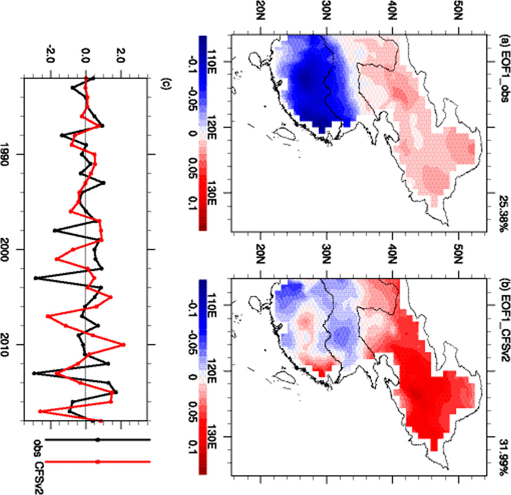
FIGURE 2. First empirical orthogonal function mode (EOF1) of summer FEHEs over eastern China in (A) the observations and (B) the CFSv2 hindcasts. (C) The standardized time series projected to the observed EOF1 of the FEHEs in the observations (black line) and the CFSv2 hindcasts (red line). The percentages in the top-right corner of (A, B) are the explained variance to the total variance.

Predictors used in the physical–empirical model for prediction of the dominant mode

Our previous studies have analyzed the mechanism associated with the dominant mode of the FEHEs over eastern China (Zhu et al., 2020a; Zhu et al., 2022). Based on these previous studies, we identified the predictors with a physical connection to the dominant mode, analyzed the corresponding mechanisms and used them to build the physical–empirical model.

Predictor in the CFSv2 hindcasts

Previous studies have shown that the SSTs in the tropical Pacific Ocean have an important role in the variation of the summer climate over East Asia (Sun and Wang 2019; Zhu et al., 2020a; Hong et al., 2022). Figure 3A shows that there were significant negative correlation coefficients between the SSTs around the maritime continent and PC1_obs. To further explore the physical relationship between them, we investigated the climate anomalies associated with the SSTs around the maritime continent and an SST index (MCSST) was defined as the areal mean SSTs within (15°S−10°N, 110–160°E) (Figure 3A). The anomalous cold SSTs around the maritime continent suppressed convection in the overlying troposphere (Figure 4A), which further led to an anomalous cyclone (anticyclone) and ascending (descending) motion over southern (northeastern) China via a meridional teleconnection similar to the Pacific–Japan/East Asia–Pacific (PJ/EAP) pattern (Nitta 1987; Huang 1992; Qiao et al., 2021). The anomalous atmospheric circulation related to the anomalous cold SSTs around the maritime continent could contribute to strengthened (weakened) convection over southern (northeastern) China (Figure 4A), leading to less (more) downward shortwave radiation (Figure 4B), which could induce less (more) FEHEs over southern (northeastern) China (Figure 4C) and contribute to the dominant mode of FEHEs (Figure 2A).

FIGURE 3

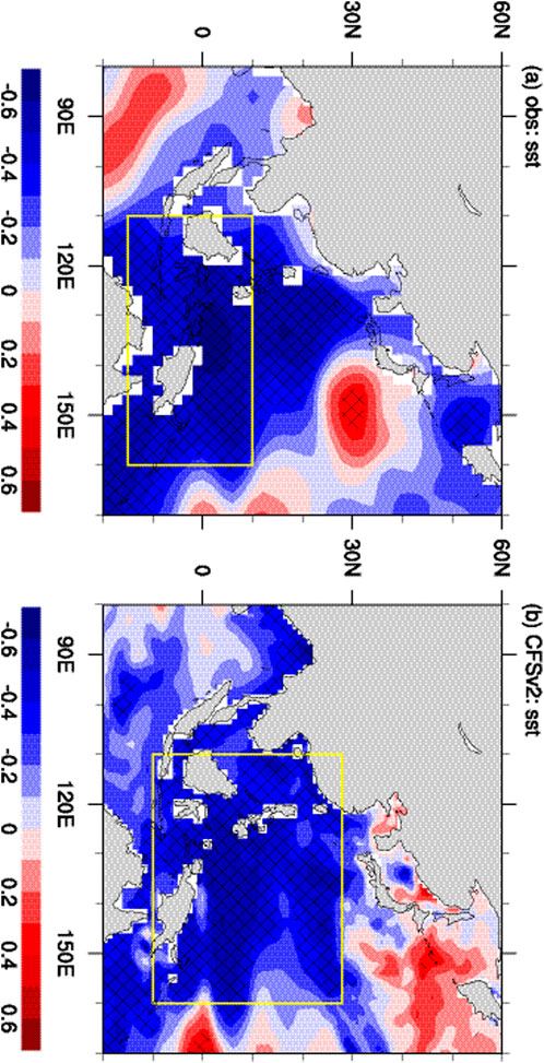
FIGURE 3. Correlation coefficients between PC1_obs and the summer SST in (A) the observations and (B) the CFSv2 hindcasts. The meshes denote the correlation coefficients significant at the 95% confidence level based on Student’s t-test.

FIGURE 4

FIGURE 4. Anomalies of the summer (A) 500 hPa vertical velocity (shading; units: 10^–3 Pa s⁻¹) and 850 hPa horizontal wind (vector; units: m s⁻¹), (B) surface net downward shortwave radiation (units: W m⁻²) and (C) FEHEs in the observations regressed on the time series of the sign-reversed MCSST. The dots denote the anomalies significant at the 90% confidence level based on Student’s t-test. Only the anomalies of the 850 hPa wind exceeding 0.1 m s⁻¹ are shown.

The PJ/EAP index, defined as the first empirical orthogonal function mode of summer 850-hPa relative vorticity within (0°−60°N, 100–160°E) according to Kosaka and Nakamura (2010), was significantly correlated with PC1_obs and sign-reversed MCSST with correlation coefficients of 0.60 and 0.51 exceeding the 99% confidence level respectively. These results indicate that the PJ/EAP teleconnection was responsible for the linkage between the dominant mode of FEHEs and the SSTs around the maritime continent. The anomalous cyclonic surface wind over the western subtropical Pacific could induce the divergence of upper water and the upwelling of cold water (figures not shown; Price et al., 1987; Seager et al., 2001), and downward shortwave radiation was reduced (Figure 4B), which could lead to negative SSTs in the western subtropical Pacific (Figure 3A). As shown in Figure 3, the physical connection between PC1_obs and the anomalous cold SSTs in the western tropical and subtropical Pacific (Figure 3A) was well revealed in the CFSv2 hindcasts (Figure 3B). The areal mean CFSv2 hindcast SSTs within (10S°−28°N, 110–160°E; Figure 3B) was abbreviated as sst_CFSv2, which was physically connected to PC1_obs with a correlation coefficient of –0.58 significant at the 99% confidence level and could be used as a predictor in the physical–empirical model to predict the dominant mode of the FEHEs over eastern China.

Predictor in the observations

Soil moisture varies slowly and has a memory of climate anomalies. It has therefore been considered as a potential predictor of extreme climate events (Wu and Zhang 2015; Yang et al., 2019). We therefore examined the connection between the preceding soil moisture and PC1_obs. Figure 5 shows that there were significant negative correlation coefficients between the soil moisture over southern China in the preceding December and PC1_obs, which lasted from the preceding December to May. However, this negative relationship (Figure 5A−F) became positive in summer (Figure 5G−I), indicating that the persistence of soil moisture could not explain the relationship between the soil moisture over southern China in the preceding December and PC1_obs. To further study the physical connection between them, we defined a soil moisture index (soil_Dec) as the preceding December soil moisture averaged within (22–30°N, 110–120°E).

FIGURE 5

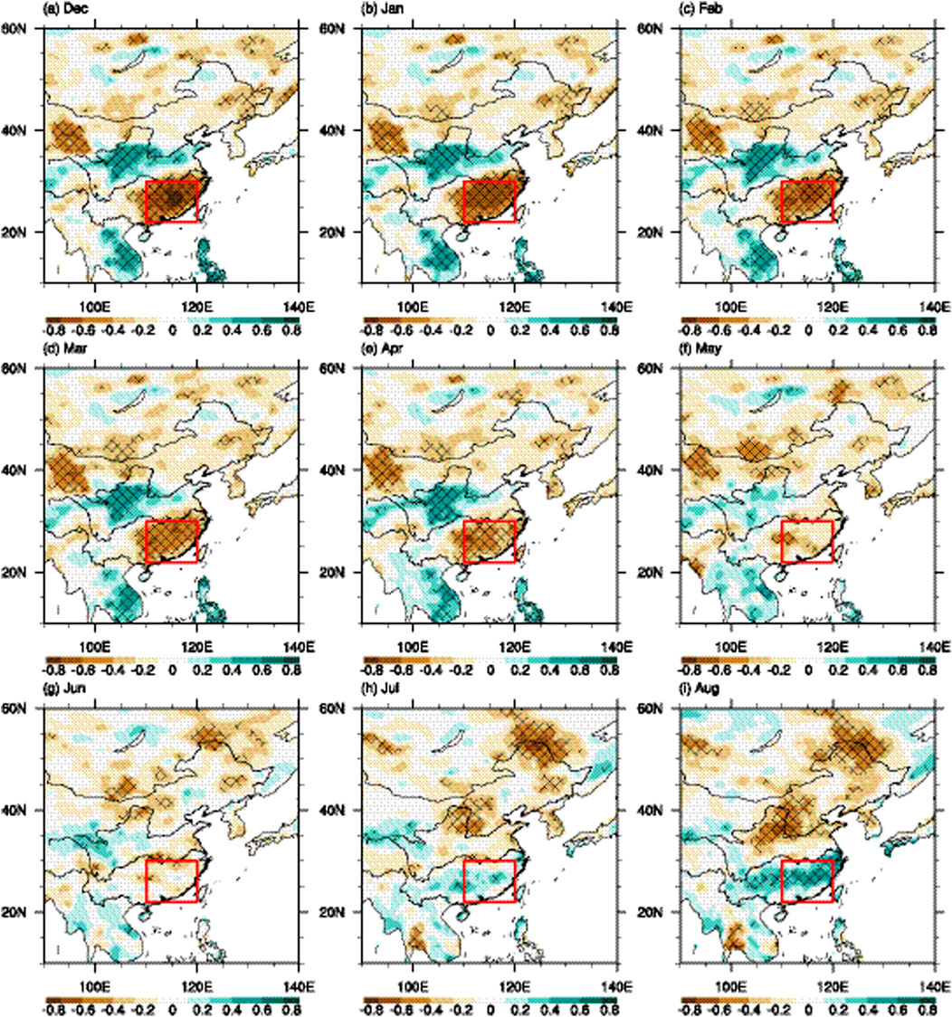
FIGURE 5. Correlation coefficients between PC1_obs and soil moisture in the preceding (A) December, (B) January, (C) February, (D) March, (E) April and (F) May and the simultaneous (G) June, (H) July and (I) August. The meshes denote the correlation coefficients significant at the 95% confidence level based on Student’s t-test.

Figure 6B shows that the deficit of soil moisture over southern China in December was associated with La Nina-like SST anomalies over the tropical Pacific. These negative SST anomalies over the eastern tropical Pacific Ocean can induce an anomalous cyclone over the western subtropical Pacific (Figure 6A) via the Pacific–East Asia teleconnection (Wang et al., 2000). The anomalous northerly wind to the west of the anomalous cyclone can suppress the transport of water vapor to southern China, inducing greater evaporation of the underlying sea surface and negative SST anomalies along the coast of southern China (Figure 6A,B). This can suppress convection and lead to the soil moisture deficit over southern China. From the preceding December to the following summer, the SST anomalies over the tropical Pacific Ocean were characterized by the decay of La Nina conditions (Figure 6B,D,F,H), with significant negative SST anomalies over the eastern tropical Pacific Ocean in December (Figure 6B) turning into positive anomalies in the following summer accompanied by negative anomalies over the western tropical Pacific Ocean (Figure 6H). The anomalous cold SSTs over the western tropical Pacific Ocean can induce anomalous descending motion over the maritime continent, which could lead to an anomalous cyclone (anticyclone) and ascending (descending) motion over southern (northeastern) China via the PJ/EAP teleconnection, contributing to the dominant mode of the FEHEs over eastern China (Figure 6G,H).

FIGURE 6

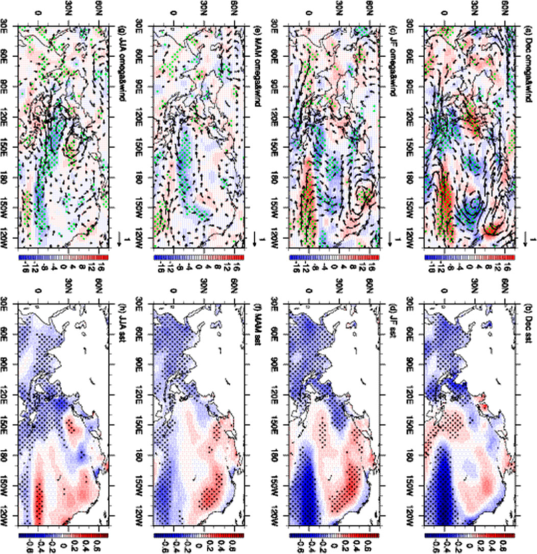
FIGURE 6. Anomalies of (A,C,E,G) the 500 hPa vertical velocity (shading; units: 10^–3 Pa s⁻¹) and 850 hPa horizontal wind (vector; units: m s⁻¹) and (B,D,F,H) the SST (units: K) in the simultaneous (A,B) December, the following (C,D) January−February mean, (E,F) March−April−May mean and (G,H) summer regressed on the time series of the sign-reversed soil_Dec. The dots denote the anomalies significant at the 90% confidence level based on Student’s t-test. Only the anomalies of 850 hPa wind exceeding 0.1 m s⁻¹ are shown.

In addition, there were negative SST anomalies in the northern Indian Ocean in December, persisting to the following summer with the decay of La Nina conditions (Figure 6B,D,F,H). This is referred to as the Indian Ocean capacitor effect and extends the influence of the ENSO into the following summer (Xie et al., 2009). The anomalous cold SSTs over the Indian Ocean during the summer can suppress convection in the overlying troposphere (Figure 6G,H), which may contribute to an anomalous cyclone over the subtropical Pacific Ocean via a Kelvin wave-induced Ekman divergence mechanism, intensifying anomalous ascending motion over southern China and the western subtropical Pacific Ocean (Figure 6G; Sun et al., 2019). Moreover, the El Nino condition in December could contribute to positive soil moisture anomalies in southern China (figure not shown), which also decayed in the following seasons. This analysis shows that the connection between the soil moisture over southern China in December and the dominant mode of the summer FEHEs can be partly attributed to their responses to the ENSO. However, the correlation coefficient between PC1_obs and Nino3.4 in December (−0.39, significant at the 90% confidence level) was lower than that between PC1_obs and soil_Dec (−0.78), indicating that other physical processes were responsible for the relationship between PC1_obs and soil_Dec.

The SST anomalies associated with soil_Dec (Figure 6B,D,F,H) and Nino3.4 in December (Figure 7) showed similarity over the tropical Pacific Ocean. By contrast, there were discrepancies over the northern extratropical Pacific Ocean, with positive anomalies over the northeastern (northern central) Pacific Ocean related to soil_Dec (Nino3.4) (Figures 6, 7), indicating the influence of air–sea interactions over the northern extratropical Pacific Ocean on soil_Dec. After removing the linear signal of Nino3.4 in December from soil_Dec, the SST anomalies associated with soil_Dec showed positive (negative) anomalies over the northeastern (northern central) Pacific Ocean (Figure 8B), enhancing (weakening) convection in the overlying troposphere (Figure 8A). An anomalous cyclone was formed over the northeastern Pacific as a Rossby wave response to the enhanced convection (Figure 8A). The anomalous cyclone induced anomalous westerly wind over the tropical and subtropical Pacific Ocean, contributing to a weakened Walker circulation, anomalous cold SSTs over the South China Sea and descending anomalies over southern China (Figures 8A,B), which favored the deficit in soil moisture over southern China.

FIGURE 7

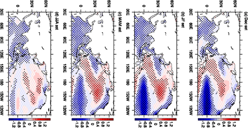
FIGURE 7. Anomalies of the SST (units: K) in the simultaneous (A) December, the following (B) January−February mean, (C) March−April−May mean and (D) summer regressed on the time series of the sign-reversed Nino3.4 in December. The dots denote the anomalies significant at the 90% confidence level based on Student’s t-test.

FIGURE 8

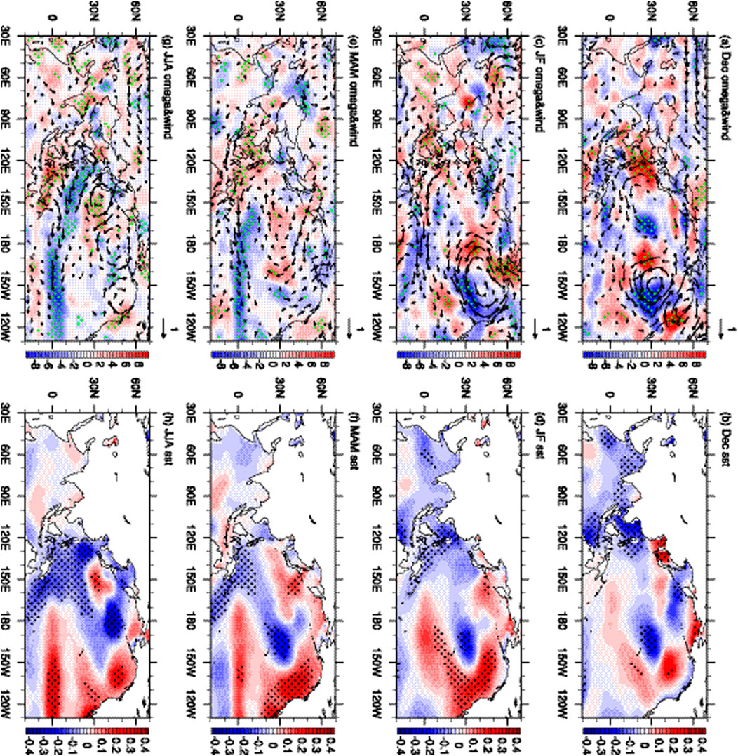
FIGURE 8. Anomalies of (A,C,E,G) the 500 hPa vertical velocity (shading; units: 10^–3 Pa s⁻¹) and 850 hPa horizontal wind (vector; units: m s⁻¹) and (B,D,F,H) the SST (units: K) in the simultaneous (A,B) December, the following (C,D) January−February mean, (E,F) March−April−May mean and (G,H) summer regressed on the time series of the sign-reversed soil_Dec with the linear signal of Nino3.4 in December removed. The dots denote the anomalies significant at the 90% confidence level based on Student’s t-test. Only the anomalies of the 850 hPa wind exceeding 0.1 m s⁻¹ are shown.

In late winter, the anomalous cyclone over the northeastern Pacific Ocean intensified and the anomalous westerly wind moved equatorward (Figure 8C), which provided favorable conditions for the developing El Niño, with negative (weak positive) SST anomalies over the western (eastern) tropical Pacific (Figure 8D). In spring, the air–sea interactions over the northeastern Pacific Ocean weakened and the anomalous cyclone disappeared (Figure 8E), but the anomalous westerly wind over the tropical Pacific Ocean lasted until summer and El Niño continued to develop via Bjerknes positive feedback (Bjerknes 1969). In summer, the anomalous cold SST over the western tropical Pacific Ocean induced anomalous descending motion over the maritime continent (Figure 8G,H), which further led to an anomalous cyclone and ascending motion over southern China and the western subtropical Pacific Ocean and exerted an influence on the dominant mode of the FEHEs over eastern China.

These results show that soil_Dec contained the signal of air–sea interactions over the tropical and northern extratropical Pacific Ocean in the preceding December, which can influence the atmospheric circulation and the dominant mode of the FEHEs over eastern China in the following summer by inducing anomalous SSTs in the Indian and tropical Pacific oceans (Figures 6-8). As a result of the combination of the signal of the air–sea interactions over the tropical and northern extratropical Pacific Ocean in the preceding December, the soil_Dec was closely correlated with PC1_obs with a correlation coefficient of −0.78 and served as a predictor in the physical–empirical model.

Establishment and estimation of the physical–empirical model

The physical–empirical model was established based on a multiple linear regression method using the sst_CFSv2 and soil_Dec predictors. Table 1 summarized the definitions of the predictors and their correlation coefficients with PC1_obs. Considering that the two predictors were not linear independent, the sst_CFSv2 with the linear signal of soil_Dec removed, was used in the physical–empirical model, which was still significantly correlated with PC1_obs at the 90% confidence level. The physical–empirical model is described as follows:

$\mathrm{P}\mathrm{C}{1}_{\mathrm{o}\mathrm{b}\mathrm{s}}=a\times {\mathrm{s}\mathrm{s}\mathrm{t}}_{\mathrm{C}\mathrm{F}\mathrm{S}\mathrm{v}2}+b\times {\mathrm{s}\mathrm{o}\mathrm{i}\mathrm{l}}_{\mathrm{D}\mathrm{e}\mathrm{c}}+c,$

where a and b are the partial regression coefficients for the predictors sst_CFSv2 and soil_Dec, respectively, and c is the intercept of PC1_obs. The values of a, b and c will be different in the different training periods.

TABLE 1

TABLE 1. Definitions of the predictors and the correlation coefficients between PC1_obs and the predictors.

The prediction of the physical–empirical model for PC1_obs was evaluated by the methods of one-year-leave cross-validation for 1982–2018 and independent hindcast for 2000–2018. The results of the one-year-leave cross-validation showed that the physical–empirical model-predicted PC1 (PC1_PE) was highly consistent with PC1_obs (Figure 9A). Compared with the prediction of CFSv2 (Figure 2C), the correlation coefficient between the PC1_PE and PC1_obs increased to 0.79, significant at the 99% confidence level, and the RMSE was reduced by 52% (Table 2). Specifically, in some extreme years (e.g., 1998 and 2003), the anomalies of PC1_obs larger than one standardized deviation were captured better by the physical–empirical mode1 than by the CFSv2 prediction (Figure 9A). Accordingly, the rate of same signs was improved from 19/37 in the CFSv2 to 30/37 in the physical–empirical model and all the signs of PC1_obs in the extreme years (the absolute value of PC1_obs larger than one standard deviation) were correctly captured in the physical–empirical model (Table 2).

FIGURE 9

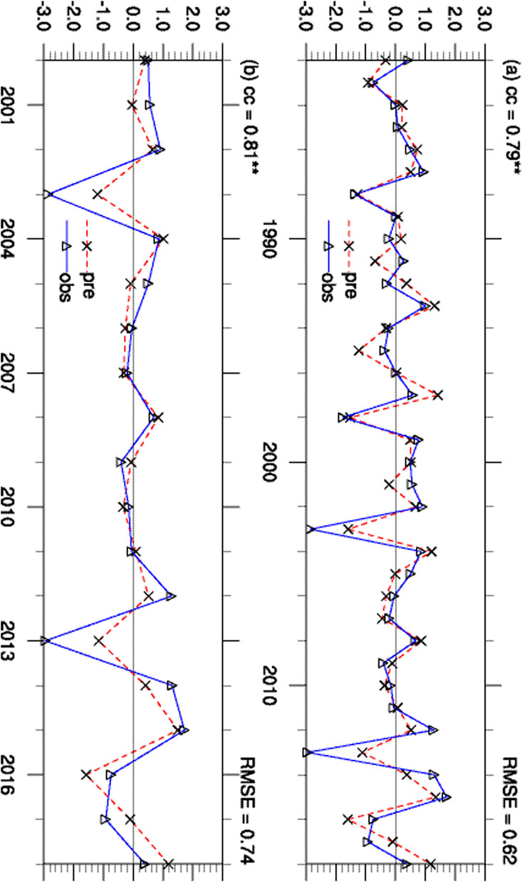
FIGURE 9. The physical–empirical model-predicted PC1 (PC1_PE, red dashed line) and PC1_obs (blue solid line) in (A) the one-year-leave cross-validation for 1982–2018 and (B) the independent hindcast for 2000–2018. The value in the top-left (top-right) corner of (A−B) is the correlation coefficient (RMSE) between PC1_PE and PC1_obs. ** denotes the correlation coefficients significant at the 99% confidence level based on Student’s t-test.

TABLE 2

TABLE 2. Correlation coefficient (CC), RMSE, the rate of same signs in all years (SS) and in extreme years (SS-extreme) between PC1_obs and PC1_CFSv2 during 1982–2018 (CC1, RMSE1, SS1 and SS1-extreme) and during 2000–2018 (CC2, RMSE2, SS2 and SS2-extreme). The correlation coefficient (CC), RMSE, the rate of same signs in all years (SS) and in extreme years (SS-extreme) between PC1_obs and PC1_PE in the one-year-leave cross validation (CC1, RMSE1, SS1 and SS1-extreme) and in the independent hindcast (CC2, RMSE2, SS2 and SS2-extreme). The bold value denotes that the correlation coefficients were significant at the 99% confidence level based on Student’s t-test.

As for the independent hindcast results (Figure 9B), the physical–empirical model also showed an improved prediction of PC1_obs compared with the prediction of the CFSv2 hindcasts (Figure 2C). The interannual variability of PC1_obs was captured well by the physical–empirical model (Figure 9B), with a correlation coefficient of 0.81 and a reduced RMSE between PC1_obs and PC1_PE (Table 2). The signs of PC1_obs were better predicted in the physical–empirical model than in the CFSv2 hindcast (Table 2). The relationship between PC1_obs and predictors was robust (figures not shown), contributing to the stability of the prediction model. The prediction skill of the physical–empirical model based on sst_CFSv2 and soil_Dec, was better than that only based on soil_Dec (figure not shown). Therefore, the physical–empirical model has the ability to improve the prediction of the dominant mode of summer FEHEs over eastern China.

Conclusion

We have shown a limited prediction capability of CFSv2 hindcasts for summer FEHEs over eastern China. The CFSv2 hindcasts did not capture the dipole pattern of the dominant mode in the observations, which was characterized by negative (positive) anomalies over southern (northeastern) China and relatively large loadings over southern China. The time series in the CFSv2 hindcasts and in the observations projected to the observed dominant mode were also inconsistent, with a low time correlation coefficient of 0.18, significant below the 90% confidence level.

To improve the prediction of the dominant mode of the FEHEs, a physical–empirical model was established based on two predictors (sst_CFSv2 and soil_Dec). The SST anomalies in the western tropical Pacific Ocean influenced convection in the overlying troposphere, affecting the atmospheric circulation over eastern China via the PJ/EAP teleconnection and contributing to the dominant mode of the FEHEs. The physical connection between the dominant mode of FEHEs and the western tropical and subtropical Pacific Ocean was well revealed in the CFSv2 hindcasts and thus the CFSv2-predicted SSTs in the western tropical and subtropical Pacific Ocean was used as the predictor sst_CFSv2. The predictor in the observations was the soil moisture over southern China in the preceding December (soil_Dec), which combined the signal of the air–sea interactions over the tropical and northern extratropical Pacific Ocean. The decaying La Nina was characterized by negative SST anomalies over the eastern tropical Pacific Ocean in December and negative SST anomalies over the western tropical Pacific and northern Indian oceans in the following summer, which contributed to the connection between the deficit in soil moisture over southern China in December and the dominant mode of the summer FEHEs over eastern China. The air–sea interactions over the northern extratropical Pacific Ocean associated with the deficit in soil moisture favored the developing El Niño and led to anomalous cold SSTs over the western tropical Pacific Ocean in the following summer, which contributed to the dominant mode of FEHEs over eastern China. The soil_Dec was physically connected to the dominant mode of FEHEs, with a significant correlation coefficient (−0.78, significant at the 99% confidence level) with PC1_obs.

The results of the one-year-leave cross-validation and independent hindcast showed that the interannual variability of PC1_obs was better captured by the physical–empirical model than by the CFSv2 hindcasts, with an improved correlation coefficient from insignificant to around 0.8 significant at the 99% confidence level, a reduction in the RMSE by about 50% and an increased rate of same signs. In extreme years (when the absolute value of PC1_obs was greater than one standard deviation), all the signs of PC1_obs were captured in the physical–empirical model. These results show that the physical–empirical model established on these two predictors significantly improved the prediction of the dominant mode of summer FEHEs over eastern China.

Data availability statement

Publicly available datasets were analyzed in this study. This data can be found here: https://data.cma.cn/data/cdcindex/cid/00f8a0e6c590ac15.html https://psl.noaa.gov/data/gridded/data.ncep.reanalysis.html https://psl.noaa.gov/data/gridded/data.noaa.ersst.v3.html https://www.ncei.noaa.gov/products/weather-climate-models/climate-forecast-system.

Author contributions

BS and HL contributed to the conception of the study. BaZ, BS, and HL contributed significantly to the analysis and preparation of the paper. BaZ performed the data analysis and wrote the paper. BS, HL, BoZ, and MD helped to edit the paper.

Funding

This study was funded by the Natural Science Foundation of China (Grants 41991283 and 42005015) and the Natural Science Foundation of Jiangsu Province of China (BK20200814).

Conflict of Interest

The authors declare that the research was conducted in the absence of any commercial or financial relationships that could be construed as a potential conflict of interest.

Publisher’s note

All claims expressed in this article are solely those of the authors and do not necessarily represent those of their affiliated organizations, or those of the publisher, the editors and the reviewers. Any product that may be evaluated in this article, or claim that may be made by its manufacturer, is not guaranteed or endorsed by the publisher.

References

Bjerknes, J. (1969). Atmospheric teleconnections from the equatorial Pacific. Mon. Weather Rev. 97, 163–172. doi:10.1175/1520-0493(1969)097<0163:atftep>2.3.co;2

CrossRef Full Text | Google Scholar

Bloomfield, P. (2004). Fourier analysis of time series: An introduction. Hoboken, New Jersey, United States: John Wiley & Sons.

Google Scholar

Borg, M. A., Xiang, J., Anikeeva, O., Pisaniello, D., Hansen, A., Zander, K., et al. (2021). Occupational heat stress and economic burden: A review of global evidence. Environ. Res. 195, 110781. doi:10.1016/j.envres.2021.110781

PubMed Abstract | CrossRef Full Text | Google Scholar

Chen, H. P., and Sun, J. Q. (2018). Projected changes in climate extremes in China in a 1.5 °C warmer world. Int. J. Climatol. 38, 3607–3617. doi:10.1002/joc.5521

CrossRef Full Text | Google Scholar

Chen, P., and Sun, B. (2020). Improving the dynamical seasonal prediction of Western Pacific warm pool sea surface temperatures using a physical–empirical model. Int. J. Climatol. 40, 4657–4675. doi:10.1002/joc.6481

CrossRef Full Text | Google Scholar

Chen, R., Wen, Z., and Lu, R. (2019). Influences of tropical circulation and sea surface temperature anomalies on extreme heat over Northeast Asia in the midsummer of 2018. Atmos. Ocean. Sci. Lett. 12, 238–245. doi:10.1080/16742834.2019.1611170

CrossRef Full Text | Google Scholar

Chen, R., Wen, Z., and Lu, R. (2018). Interdecadal change on the relationship between the mid-summer temperature in South China and atmospheric circulation and sea surface temperature. Clim. Dyn. 51, 2113–2126. doi:10.1007/s00382-017-4002-5

CrossRef Full Text | Google Scholar

Deng, K., Yang, S., Ting, M., Zhao, P., and Wang, Z. (2019). Dominant modes of China summer heat waves driven by global sea surface temperature and atmospheric internal variability. J. Clim. 32, 3761–3775. doi:10.1175/jcli-d-18-0256.1

CrossRef Full Text | Google Scholar

Gao, M., Wang, B., Yang, J., and Dong, W. (2018). Are peak summer sultry heat wave days over the Yangtze–Huaihe River basin predictable? J. Clim. 31, 2185–2196. doi:10.1175/jcli-d-17-0342.1

CrossRef Full Text | Google Scholar

Han, T., Li, S., Hao, X., and Guo, X. (2020). A statistical prediction model for summer extreme precipitation days over the northern central China. Int. J. Climatol. 40, 4189–4202. doi:10.1002/joc.6451

CrossRef Full Text | Google Scholar

Hong, H., Sun, J., and Wang, H. (2020). Interdecadal variation in the frequency of extreme hot events in Northeast China and the possible mechanism. Atmos. Res. 244, 105065. doi:10.1016/j.atmosres.2020.105065

CrossRef Full Text | Google Scholar

Hong, H., Sun, J., and Wang, H. (2022). Variations in summer extreme high-temperature events over northern Asia and the possible mechanisms. J. Clim. 35, 335–357. doi:10.1175/JCLI-D-21-0043.1

CrossRef Full Text | Google Scholar

Huang, B., Thorne, P. W., Banzon, V. F., Boyer, T., Zhang, H. M., Lawrimore, J. H., et al. (2017). Extended reconstructed sea surface temperature, version 5 (ERSSTv5): Upgrades, validations, and intercomparisons. J. Clim. 30, 8179–8205. doi:10.1175/jcli-d-16-0836.1

CrossRef Full Text | Google Scholar

Huang, J., van den Dool, H. M., and Georgakakos, K. G. (1996). Analysis of model-calculated soil moisture over the United States (1931–1993) and applications to long-range temperature forecasts. J. Clim. 9, 1350–1362. doi:10.1175/1520-0442(1996)009<1350:aomcsm>2.0.co;2

CrossRef Full Text | Google Scholar

Huang, R. (1992). The East Asia/Pacific pattern teleconnection of summer circulation and climate anomaly in East Asia. J. Meteorological Res. 6, 25–37.

Google Scholar

Igun, E., Xu, X., Hu, Y., and Jia, G. (2022). Strong heatwaves with widespread urban-related hotspots over Africa in 2019. Atmos. Ocean. Sci. Lett. 15, 100195. doi:10.1016/j.aosl.2022.100195

CrossRef Full Text | Google Scholar

Ji, L., and Fan, K. (2019). Climate prediction of dust weather frequency over northern China based on sea-ice cover and vegetation variability. Clim. Dyn. 53, 687–705. doi:10.1007/s00382-018-04608-w

CrossRef Full Text | Google Scholar

Kalnay, E., Kanamitsu, M., Kistler, R., Collins, W., Deaven, D., Gandin, L., et al. (1996). The NCEP/NCAR 40-year reanalysis project. Bull. Am. Meteorol. Soc. 77, 437–471. doi:10.1175/1520-0477(1996)077<0437:tnyrp>2.0.co;2

CrossRef Full Text | Google Scholar

Kosaka, Y., and Nakamura, H. (2010). Mechanisms of meridional teleconnection observed between a summer monsoon system and a subtropical anticyclone. Part I: The Pacific–Japan pattern. J. Clim. 23, 5085–5108. doi:10.1175/2010jcli3413.1

CrossRef Full Text | Google Scholar

Li, H., Chen, H., Wang, H., Sun, J., and Ma, J. (2018). Can Barents Sea ice decline in spring enhance summer hot drought events over northeastern China? J. Clim. 31, 4705–4725. doi:10.1175/jcli-d-17-0429.1

CrossRef Full Text | Google Scholar

Li, M., Luo, D., Yao, Y., and Zhong, L. (2020). Large-scale atmospheric circulation control of summer extreme hot events over China. Int. J. Climatol. 40, 1456–1476. doi:10.1002/joc.6279

CrossRef Full Text | Google Scholar

Liu, W., Chen, R., and Wen, Z. (2021). An interdecadal decrease in extreme heat days in August over Northeast China around the early 1990s. Atmos. Ocean. Sci. Lett. 14, 100001. doi:10.1016/j.aosl.2020.100001

CrossRef Full Text | Google Scholar

Long, Y., Li, J., Zhu, Z., and Zhang, J. (2022). Predictability of the anomaly pattern of summer extreme high-temperature days over southern China. Clim. Dyn. 59, 1027–1041. doi:10.1007/s00382-022-06170-y

CrossRef Full Text | Google Scholar

Luo, N., Guo, Y., Gao, Z., Chen, K., and Chou, J. (2020). Assessment of CMIP6 and CMIP5 model performance for extreme temperature in China. Atmos. Ocean. Sci. Lett. 13, 589–597. doi:10.1080/16742834.2020.1808430

CrossRef Full Text | Google Scholar

Nitta, T. (1987). Convective activities in the tropical Western Pacific and their impact on the Northern Hemisphere summer circulation. J. Meteorological Soc. Jpn. 65, 373–390. doi:10.2151/jmsj1965.65.3_373

CrossRef Full Text | Google Scholar

North, G. R., Bell, T. L., Cahalan, R. F., and Moeng, F. J. (1982). Sampling errors in the estimation of empirical orthogonal functions. Mon. Weather Rev. 110, 699–706. doi:10.1175/1520-0493(1982)110<0699:seiteo>2.0.co;2

CrossRef Full Text | Google Scholar

Orlowsky, B., and Seneviratne, S. I. (2012). Global changes in extreme events: Regional and seasonal dimension. Clim. Change 110, 669–696. doi:10.1007/s10584-011-0122-9

CrossRef Full Text | Google Scholar

Pepler, A. S., Díaz, L. B., Prodhomme, C., Doblas-Reyes, F. J., and Kumar, A. (2015). The ability of a multi-model seasonal forecasting ensemble to forecast the frequency of warm, cold and wet extremes. Weather Clim. Extrem. 9, 68–77. doi:10.1016/j.wace.2015.06.005

CrossRef Full Text | Google Scholar

Price, J. F., Weller, R. A., and Schudlich, R. R. (1987). Winddriven ocean currents and Ekman transport. Science 238, 1534–1538. doi:10.1126/science.238.4833.1534

PubMed Abstract | CrossRef Full Text | Google Scholar

Qiao, S., Chen, D., Wang, B., Cheung, H., Liu, F., Cheng, J., et al. (2021). The longest 2020 Meiyu season over the past 60 years: Subseasonal perspective and its predictions. Geophys. Res. Lett. 48, e2021GL093596. doi:10.1029/2021gl093596

CrossRef Full Text | Google Scholar

Ren, L., Zhou, T., and Zhang, W. (2020). Attribution of the record-breaking heat event over northeast Asia in summer 2018: The role of circulation. Environ. Res. Lett. 15, 054018. doi:10.1088/1748-9326/ab8032

CrossRef Full Text | Google Scholar

Saha, S., Moorthi, S., Wu, X., Wang, J., Becker, E., Tripp, P., et al. (2014). The NCEP climate forecast system version 2. J. Clim. 27, 2185–2208. doi:10.1175/jcli-d-12-00823.1

CrossRef Full Text | Google Scholar

Seager, R., Kushnir, Y., Naik, N. H., Cane, M. A., and Miller, J. (2001). Wind-driven shifts in the latitude of the Kuroshio–Oyashio Extension and generation of SST anomalies on decadal timescales. J. Clim. 14, 4249–4265. doi:10.1175/1520-0442(2001)014<4249:wdsitl>2.0.co;2

CrossRef Full Text | Google Scholar

Sun, B., Li, H., and Zhou, B. (2019). Interdecadal variation of Indian Ocean basin mode and the impact on Asian summer climate. Geophys. Res. Lett. 46, 12388–12397. doi:10.1029/2019gl085019

CrossRef Full Text | Google Scholar

Sun, B., and Wang, H. (2019). Enhanced connections between summer precipitation over the Three-River-Source region of China and the global climate system. Clim. Dyn. 52, 3471–3488. doi:10.1007/s00382-018-4326-9

CrossRef Full Text | Google Scholar

Sun, Y., Zhang, X. B., Zwiers, F. W., Song, L. C., Wan, H., Hu, T., et al. (2014). Rapid increase in the risk of extreme summer heat in Eastern China. Nat. Clim. Chang. 4, 1082–1085. doi:10.1038/nclimate2410

CrossRef Full Text | Google Scholar

Tang, S., Qiao, S., Feng, T., Jia, Z., Zang, N., and Feng, G. (2021a). Predictability of the mid-summer surface air temperature over the yangtze river valley in the national centers for environmental prediction climate forecast system. Int. J. Climatol. 41, 811–829. doi:10.1002/joc.6670

CrossRef Full Text | Google Scholar

Tang, S., Qiao, S., Feng, T., Wang, Y., Yang, Y., Zhang, Z., et al. (2021b). Asymmetry of probabilistic prediction skills of the midsummer surface air temperature over the middle and lower reach of the Yangtze River valley. Clim. Dyn. 57, 3285–3302. doi:10.1007/s00382-021-05866-x

CrossRef Full Text | Google Scholar

Tian, B., and Fan, K. (2020). Climate prediction of summer extreme precipitation frequency in the Yangtze River valley based on sea surface temperature in the southern Indian Ocean and ice concentration in the Beaufort Sea. Int. J. Climatol. 40, 4117–4130. doi:10.1002/joc.6446

CrossRef Full Text | Google Scholar

Tong, Q., Huang, Y., Duan, M., and Zhao, Q. (2020). Possible contribution of the PDO to the eastward retreat of the Western Pacific subtropical high. Atmos. Ocean. Sci. Lett. 14, 100005. doi:10.1016/j.aosl.2020.100005

CrossRef Full Text | Google Scholar

Wang, B., Wu, R., and Fu, X. (2000). Pacific–East asian teleconnection: How does ENSO affect East asian climate? J. Clim. 13, 1517–1536. doi:10.1175/1520-0442(2000)013<1517:peathd>2.0.co;2

CrossRef Full Text | Google Scholar

WMO (2013). The global climate 2001–2010: A decade of climate extremes. Geneva, Switzerland: World Meteorological Organization Rep. WMO-1103, 110.

Google Scholar

Wu, J., and Gao, X. J. (2013). A gridded daily observation dataset over China region and comparison with the other datasets. Chin. J. Geophys. 56, 1102–1111. in Chinese. doi:10.6038/cjg20130406

CrossRef Full Text | Google Scholar

Wu, L., and Zhang, J. (2015). The relationship between spring soil moisture and summer hot extremes over North China. Adv. Atmos. Sci. 32, 1660–1668. doi:10.1007/s00376-015-5003-0

CrossRef Full Text | Google Scholar

Xie, S., Hu, K., Hafner, J., Tokinaga, H., Du, Y., Huang, G., et al. (2009). Indian Ocean capacitor effect on Indo–Western Pacific climate during the summer following El Niño. J. Clim. 22, 730–747. doi:10.1175/2008jcli2544.1

CrossRef Full Text | Google Scholar

Xu, K., Lu, R., Mao, J., and Chen, R. (2019). Circulation anomalies in the mid–high latitudes responsible for the extremely hot summer of 2018 over northeast Asia. Atmos. Ocean. Sci. Lett. 12, 231–237. doi:10.1080/16742834.2019.1617626

CrossRef Full Text | Google Scholar

Yang, K., Zhang, J., Wu, L., and Wei, J. (2019). Prediction of summer hot extremes over the middle and lower reaches of the Yangtze River valley. Clim. Dyn. 52, 2943–2957. doi:10.1007/s00382-018-4302-4

CrossRef Full Text | Google Scholar

Yang, Y., Lin, Z., Luo, L., Zhang, Y., and Li, Z. (2021). Inhomogeneous trends in the onset date of extreme hot days in China over the last five decades. Atmos. Ocean. Sci. Lett. 14, 100080. doi:10.1016/j.aosl.2021.100080

CrossRef Full Text | Google Scholar

You, Q. L., Jiang, Z. H., Kong, L., Wu, Z. W., Bao, Y. T., Kang, S. C., et al. (2017). A comparison of heat wave climatologies and trends in China based on multiple definitions. Clim. Dyn. 48, 3975–3989. doi:10.1007/s00382-016-3315-0

CrossRef Full Text | Google Scholar

Zhang, D., Huang, Y., Sun, B., Li, F., and Wang, H. (2019b). Verification and improvement of the ability of CFSv2 to predict the Antarctic Oscillation in boreal spring. Adv. Atmos. Sci. 36, 292–302. doi:10.1007/s00376-018-8106-6

CrossRef Full Text | Google Scholar

Zhang, D., Huang, Y., and Sun, B. (2019a). Verification and improvement of the capability of ensembles to predict the winter arctic oscillation. Earth Space Sci. 6, 1887–1899. doi:10.1029/2019ea000771

CrossRef Full Text | Google Scholar

Zhang, Y., Zhou, W., and Leung, M. (2019c). Phase relationship between summer and winter monsoons over the South China sea: Indian Ocean and ENSO forcing. Clim. Dyn. 52, 5229–5248. doi:10.1007/s00382-018-4440-8

CrossRef Full Text | Google Scholar

Zhou, Y., Yuan, J., Wen, Z., Huang, S., Chen, X., Guo, Y., et al. (2022). The impacts of the East Asian subtropical westerly jet on weather extremes over China in early and late summer. Atmos. Ocean. Sci. Lett. 15, 100212. doi:10.1016/j.aosl.2022.100212

CrossRef Full Text | Google Scholar

Zhu, B., Sun, B., Li, H., and Wang, H. (2020b). Interdecadal variations in extreme high-temperature events over southern China in the early 2000s and the influence of the Pacific Decadal Oscillation. Atmosphere 11, 829. doi:10.3390/atmos11080829

CrossRef Full Text | Google Scholar

Zhu, B., Sun, B., and Wang, H. (2020a). Dominant modes of interannual variability of extreme high‐temperature events in eastern China during summer and associated mechanisms. Int. J. Climatol. 40, 841–857. doi:10.1002/joc.6242

CrossRef Full Text | Google Scholar

Zhu, B., Sun, B., and Wang, H. (2022). Increased interannual variability in the dipole mode of extreme high-temperature events over east China during summer after the early 1990s and associated mechanisms. J. Clim. 35, 1347–1364. doi:10.1175/jcli-d-21-0431.1

CrossRef Full Text | Google Scholar