Remote sensing image classification based on object-oriented convolutional neural network

Remote sensing image classification is of great importance for urban development and planning. The need for higher classification accuracy has led to improvements in classification technology. In this research, Landsat 8 images are used as experimental data, and Wuhan, Chengde and Tongchuan are selected as research areas. The best neighborhood window size of the image patch and band combination method are selected based on two sets of comparison experiments. Then, an object-oriented convolutional neural network (OCNN) is used as a classifier. The experimental results show that the classification accuracy of the OCNN classifier is 6% higher than that of an SVM classifier and 5% higher than that of a convolutional neural network classifier. The graph of the classification results of the OCNN is more continuous than the plots obtained with the other two classifiers, and there are few fragmentations observed for most of the category. The OCNN successfully solves the salt and pepper problem and improves the classification accuracy to some extent, which verifies the effectiveness of the proposed object-oriented model.

1 Introduction

Global change has always been an important area of remote sensing research in terms of socioeconomic and ecological environments (Linda et al., 2015; L Turner et al., 2008). To monitor global change, we must obtain a large amount of data, and land cover data are among the most important. Land cover data are the basis of many studies on land resource management, ecological health and sustainable development (Foley et al., 2005; Lu and Weng, 2007; Sterling et al., 2012). Remote sensing images with high temporal resolution, high spatial resolution and high spectral resolution over large geographical areas provide a sufficient basis for the acquisition of land cover data (Li et al., 2014). With the evolution of classification methods, remote sensing technology has become a powerful way to obtain land use data (Rogan and Chen, 2004; Huang and Jia, 2012). As more land cover data have been produced, it has become necessary to ensure the accuracy and availability of land classification products.

At present, the methods of classifying remote sensing images can be divided into three types: visual interpretation (Yang et al., 2011), traditional pattern classification (Zhihong and Xingwan, 2014) and neural network classification (Huang et al., 2018). The accuracy of visual interpretation is generally higher than that of computer classification, but the labor cost is high, thus limiting this approach in large-scale remote sensing research. Methods of traditional pattern classification use classifier algorithms to perform automatic category interpretation with remote sensing images. A classification method with pixels as the basic classification unit assumes that each pixel represents only one type of land cover. In general, pixel classification algorithms can be divided into unsupervised classification and supervised classification methods. Unsupervised classification does not require prior knowledge (Puletti et al., 2014), and corresponding methods include the k-means (Blanzieri and Melgani, 2008) algorithm and ISODATA clustering algorithm (Hong et al., 2016). However, unsupervised classification requires the postprocessing and analysis of the classified results. In comparison, supervised classification requires prior knowledge, and there are two types of classifiers used for classification: parametric classifiers and nonparametric classifiers. Parametric classifiers require the data to be normally distributed, and they include the maximum likelihood classifier (Mather, 1985) and the minimum distance-to-means classifier (Sekovski et al., 2014). However, traditional parameter classifiers do not provide high classification accuracy in complex surface environments. In contrast, nonparametric classifiers not only do not require the data to conform to a normal distribution but also effectively use nonspectral data. Studies have shown that nonparametric classifiers can achieve higher classification accuracy than parametric classifiers in complex surface environments (Foody, 2002; Murthy et al., 2003). The most commonly used nonparametric classifiers include support vector machine classifiers (Camps-Valls et al., 2003) and decision tree classifiers (Belward and Hoyos, 1987; Zhao et al., 2014). However, pixel-based classification methods may neglect the associations among objects and not utilize the spatial features of objects; thus, objects with the same spectral characteristics cannot be effectively classified (Lee et al., 2003). In comparison, the object-oriented classification method overcomes the limitation of pixel-based classification and divides images into homogeneous objects through multiscale segmentation and other image segmentation methods; in this case, object pixels are regarded as belonging to the same category (Blaschke et al., 2000; Yang et al., 2008). Using an object as a basic classification unit can not only enhance the use of the spectral features of the image but also fully consider shape features, geometric structures, texture features and context information (Yu et al., 2006; Su et al., 2008). However, both pixel-based and object-oriented classification methods cannot accurately represent the distribution of complex geographical objects due to the limitations of computing units, experimental samples and algorithm parameters. Determining how to use certain features to classify an image is currently a key problem in remote sensing image classification. Deep learning is a method that can effectively combine low-level features to form abstract high-level features and achieve learning goals (Dang et al., 2017). Convolutional neural networks (CNNs) are the most commonly used models for deep learning in image processing, and they provide more powerful feature learning and feature expression capabilities than do traditional machine learning methods (Hinton and Salakhutdinov, 2006).

The first CNN was LeNet-5 (LeCun et al., 1989), and the CNN architecture consists of convolutional layers, pooled layers, and fully connected layers. However, the activation function used by the traditional CNNs is generally a sigmoid or tanh function. If the network depth increases, the vanishing gradient problem occurs, which causes the classification accuracy of the CNN to be low. The AlexNet model proposed by the Hinton team overcame this issue, and its accuracy was 10% higher than that of the second-place support vector machine classification algorithm (Krizhevsky et al., 2012). The AlexNet model uses a ReLU function as the activation function to solve the vanishing gradient problem and uses a dropout algorithm to solve the overfitting problem to enhance model depth (Krizhevsky et al., 2012). Since AlexNet was first developed, VGG-16 (Simonyan and Zisserman, 2014), GoogLeNet (Szegedy et al., 2015) and ResNet (He et al., 2016) have been proposed, and the classification accuracy has continuously improved; these results suggest that CNNs have good application prospects in the field of image analysis. Consequently, researchers have applied CNNs in the field of remote sensing image classification. CNN classifiers generally perform better than SVM classifiers and KNN classifiers in the classification of hyperspectral images (Wei et al., 2015; Yu et al., 2017). Moreover, CNNs can extract features better than can PCA, factor analysis (FA), and local linear embedding (LLE) methods (Chen et al., 2016). CNNs can also be combined with other classifier methods to achieve high classification accuracy (Zhang et al., 2018a). The abovementioned experiments verified the feasibility of using CNNs in the classification of high-resolution remote sensing images. CNNs are used not only for the detection of objects such as airplanes (Mash et al., 2016), oil tanks (Wang et al., 2017), and airports (Peng et al., 2016) but also for the extraction of roads (Xu et al., 2018), buildings (Yang et al., 2018), and water bodies (Wei et al., 2018). However, for moderate-resolution images, the boundary of an image is difficult to distinguish with the naked eye, which causes the boundary to be blurred; as a result, the classification result is influenced by salt and pepper noise issues.

The object-oriented approach can solve this salt and pepper problem to a certain extent (Sun et al., 2010). It divides images into homogeneous objects through multiscale segmentation and other image segmentation methods (Blaschke et al., 2000; Yang et al., 2008). This type of method can not only enhance the use of the spectral features of the image but also fully consider shape features, geometric structures, texture features and context information (Yu et al., 2006; Su et al., 2008). However, it is difficult to decide how to use certain features. Convolutional neural networks (CNNs) are the most commonly used models for deep learning in image processing, and they provide more powerful feature learning and feature expression capabilities (Hinton and Salakhutdinov, 2006). So, if we combine object-oriented classification methods and CNNs for image classification, it will give full play to the advantages of CNNs method, overcome the defects of object-oriented classification method, and obtain better segmentation results.

Based on the above analysis, we propose to combine object-oriented classification methods and CNNs for moderate-resolution image classification. Wuhan, Tongchuan and Chengde are selected as the research areas. We seek to verify that the object-oriented CNN classification method has advantages in mitigating boundary blur and salt and pepper problems in Landsat 8 image classification. Therefore, experiments are designed to address the following three factors: 1) the influence of different input channels on the accuracy of model classification; 2) the influence of different neighborhood windows on the accuracy of model classification; and 3) whether the proposed object-oriented CNN can improve the accuracy of classification.

2 Methodology

2.1 Convolutional neural network

2.1.1 Convolution and pooling

The neural network described in Section 2.1 is a fully connected network in which neurons are densely connected. In the deep neural network model, if the parameters of the network structure grow exponentially, the GPU and memory may become overloaded, and even the computer running the model may crash. In contrast, CNNs greatly reduce the size of parameters and are widely used in the field of image processing. The core of a CNN is the convolutional layer. The feature value at location (i, j) in the k-th feature map $z_{i,j,k}$ is calculated by (Gu et al., 2015):

${\text{Z}}_{i,j,k}=W_k^T{X}_{i,j}^L+b_k(1)$

However, not all features extracted by the convolutional layer are useful features, and there may be a large amount of noise in the output. Therefore, the pooling layer is used to filter noise and useless features. Two types of pooling are commonly used: maximum pooling and average pooling. Average pooling is used to calculate the average in a feature map area, and the maximum pooling operation finds the maximum value in an of a feature map (Zeiler and Fergus, 2013). The pooling approach used in this paper is maximum pooling with a stride size of 2 pixels.

${\text{Z}}_{i,j}=\frac{1}{C^2}\left({\displaystyle \sum _{i=0}^c{\displaystyle \sum _{j=0}^c{X}_{i,j}}}\right)+b(2)$

${\text{Z}}_{i,j}=\underset{i=0,j=0}{\overset{c}{\max }}\left(X_{i,j}\right)+b(3)$

2.1.2 ReLU function

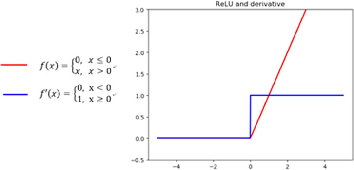
The basis of network stacking is matrix multiplication, which involves the linear transformation of a matrix. A model that includes a stacked multilayer network is essentially a linear model and cannot solve nonlinear problems. To solve complex practical problems, after each convolution layer, an activation function is added to ensure the nonlinearity of the model. However, the tanh function and the sigmoid function are prone to vanishing gradient issues (Glorot et al., 2010). To solve this problem, the ReLU function was proposed (Nair and Hinton, 2010). The definition of this function is given in Figure 1. Notably, when the input is greater than 0, the output value is unchanged, and the derivative is constant. The ReLU function can effectively alleviate the vanishing gradient problem. The ReLU function is easy to use in derivative calculations, can reduce the number of calculations, and has a much faster convergence speed than the two functions noted above. Therefore, this paper uses a ReLU activation function.

FIGURE 1

FIGURE 1. ReLU function.

2.1.3 GoogLeNet

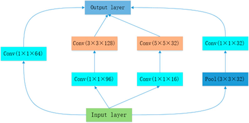
In 2014, GoogLeNet won the ILSVRC competition with a 6.5% TOP5 error rate, which was 1.3% higher than that of the second-place algorithm. The most prominent feature of GoogLeNet is a new Inception architecture. The structure shown in Figure 2 is GoogLeNet’s first Inception architecture (Szegedy et al., 2015). The core objectives are to extract image information at different scales by using multidimensional convolution kernels and then perform convolutional layer fusion to effectively extract features. The GoogLeNet model is five layers deeper than VGG-16, but fewer parameters are required. Notably, with the improved Inception architecture, GoogLeNet uses a 1×1 convolution kernel for dimensionality reduction. In each Inception structure, a maximum pooling layer is added to filter the upper layer features. The reason why the Inception architecture is successful is that a 1 × 1 convolution kernel can remove most of the sparse neurons, making the network structure more compact for extracting and filtering the features in different ranges of receptive fields. These neurons undergo amplification and recombination in the next layer without affecting the expression of the main features.

FIGURE 2

FIGURE 2. Inception structure.

2.1.4 Modified GoogLeNet

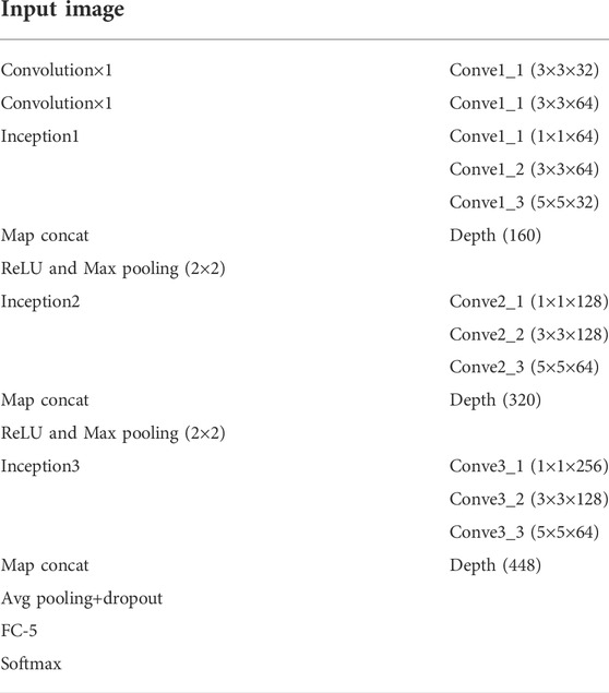
The modified GoogLeNet in this paper, as shown in Table 1, directly uses a 3×3 convolution kernel in the first two layers of the network for feature extraction. Then, we design three inception modules, each of which includes three convolution layers. Each convolution layer uses 1 × 1, 3 × 3, and 5 × 5 convolution kernels. At the end of each Inception structure, the features extracted by the three convolution kernels are fused, and the fused features are activated. After the fully connected layer, a dropout method is used. The whole model consists of 12 layers of convolution and 1 fully connected layer. The differences between the proposed model and the original model are that there is no pooling layer in the Inception module in this case and the network depth is reduced.

TABLE 1

TABLE 1. GoogLeNet-12.

To analyze the effects of different input channels and different sizes of neighborhood windows on the classification results, the following comparative experiments are designed. In the input channel experiment, channel 1 includes the true-color 3-band image, channel 2 is the true-color three-feature-band result obtained by PCA (Yang and Du, 2017), channel 3 is a true color band for the normalized difference vegetation index (NDVI), normalized difference build-up index (NDBI) and normalized difference water index (NDWI) (McFEETERS, 1996; Jakubauskas et al., 2002; Zha et al., 2003), and channel 4 consists of three feature bands obtained by PCA and three feature index bands. The size of the neighborhood window is 11 × 11. In the neighborhood window experiment, four windows of 21 × 21, 15 × 15, 11 × 11, and 7 × 7 were selected, and the channel for input data was selected as channel 4.

2.2 Object-Oriented Convolutional Neural Network

The traditional convolutional neural network model is influenced by salt and pepper problems and boundary ambiguity problems. Object-oriented classification can combine similar pixels, distinguish objects based on different features, and solve problems associated with mixed pixels and different objects with the same spectral characteristics to a certain extent. Therefore, this paper uses a combination of an object-oriented method and a CNN model to mitigate salt and pepper effects and boundary blurring.

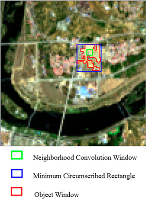
In the traditional neural network method, the input image is a fixed-dimension image, but the object of segmentation has an indefinite dimension, and the indefinite-shape image cannot be directly used as the original input of the neural network. There are two different input windows that are used to solve the input problem. As shown in Figure 3, the green window is the original CNN input window, and the size is 11 × 11; additionally, the red window is the object window, and the blue window is the minimum outer rectangle of the object.

FIGURE 3

FIGURE 3. Object-oriented convolutional neural network.

In this paper, the original CNN model is used to calculate the category of each pixel for an object, and an inverse distance weighting method is proposed. As shown in formula 2.14, the corresponding weight is determined according to the distance between each pixel and the center pixel. If the selected pixel is the central pixel itself, the weight is 1, and the farther away from the center pixel a pixel is, the smaller the weight. After calculating the weight of each pixel class for a given object, weighted statistics are used as the weight values of the green window for each category.

$q\left(x,y\right)=\{\begin{array}{cc}\frac{1}{\sqrt{{\left(x-x_0\right)}^2+{\left(y-y_0\right)}^2}}& \left(x\ne x_0,y\ne {\text{y}}_0\right)\\ 1& \left(x=x_0,y=y_0\right)\end{array}(4)$

To fully use the internal features of objects, this paper uses the red window to select internal features. First, all the pixels in the object are combined into a one-dimensional vector, and then the one-dimensional vector is equally divided. Finally, the equal-length sets are used as the inputs of the network. The specific steps are as follows.

1) First, the number of pixels associated with each object in the training dataset is determined, and the object containing the fewest pixels is identified. The minimum number of object pixels in 40 training images is 5 based on 80 segmentation scales. Therefore, the number of pixels input is set to five.

2) Channel experiments show that the three characteristic bands of PCA and the three normalized exponential bands yield the highest classification accuracy for input images. Therefore, these six channels are used to obtain image inputs for the red window approach. Then, the mean and variance of the five pixels are calculated to obtain the mean and variance of the six channels. The five pixel values and two statistical values are combined into a 7-dimensional vector, and a 42-dimensional vector is obtained by splicing with six-channel image metadata.

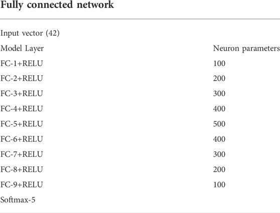
3) This paper designs a 9-layer fully connected network model to process each object, and the network structure is shown in Table 2. There are 100 neurons in the first layer. The number of neurons increases in proportion to the number of layers, and the fifth layer has 500 neurons. Additionally, a symmetrical structure is established, with 100 neurons in the ninth layer. Finally, the Softmax function is used to obtain 5 categories.

4) The first three steps are repeated until all the pixels associated with an object are classified. Redundant pixels are directly discarded, and the classification result is obtained for whole objects and input it into the fully connected model to obtain the classification result. Then, a statistical analysis of the classification result is performed to obtain the weight value for the red window.

TABLE 2

TABLE 2. Fully connected neural network.

Finally, the category of the object is determined based on the maximum value of the weights obtained by the superposition of red window and green window weights.

3 Experiment analysis

3.1 Dataset and preprocessing

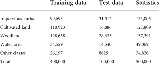
The research data used in this paper include images collected with the moderate-resolution satellite Landsat8 and provided through a geospatial data cloud platform. The research areas include Wuhan City, Hubei Province, on 9 November 2017; Tongchuan City, Shaanxi Province, on 17 April 2017; and Chengde City, Hebei Province, on 1 June 2017. To satisfy the data input format requirements for the CNN, the images of the study area are preprocessed. First, the image of each region is cut into 100 *100 pixel-size image blocks. Fifty images were selected from the clipped images, including 30 images of Wuhan, 10 images of Chengde and 10 images of Tongchuan. Forty of the 50 images were selected as training data, and 10 were selected as test data. Then, Ecognition software was used to label the types of objects in the experimental area, and 80% of the objects were manually selected. On this basis, the K-NN algorithm was used to classify the objects and use them as training labels. The experimental area was divided into five categories: impervious surface, woodland, cultivated land, water area and others. The number of pixels in each category is shown in Table 3. Because the size of the resulting images was several pixels smaller than that of the images used for labeling, a layer of padding was added to the original convolution result. The padding amount was the convolution window size minus one, and the pixel value was equal to the nearest cell size.

TABLE 3

TABLE 3. Pixel statistics for the sample set.

As shown in Figure 4, to explore the classification effects of different input bands, the four channel combinations discussed in are used to obtain four TIFF file datasets as the inputs of the model. Then, the experimental samples are transformed into TFrecord format and used as the original training data, and the results of visual interpretation are used as the training labels.

FIGURE 4

FIGURE 4. Map of the experimental area. (A) True color. (B) PCA. (C) NDVI. (D) NDWI. (E) NDBI.

The experimental environment used in this paper is as follows: Core i7-8700 (3.7 GHz) processor, 16G memory, Nvidia GeForce GTX 1070 Ti (8G) memory, Windows 10 operating system, Python 3.6, the in-depth learning framework TensorFlow 1.7, and the Python numpy scientific computing library.

3.2 Channel and window comparison experiment

As noted in Section 2.1.3 four different input channels are selected for image classification and assessed. Figure 6 is the true color image and the classification result obtained with channels 1, 2, 3, and 4 (from left to right). As shown in Figure 5, the classification results of the four input channels all exhibit fine-scale fragments. The classification results for the terrain aggregation area are obviously better than those for the area with scattered objects. The classification results for the water area class in the figure are better than those for other classes, although the ships in the water areas are misclassified as impervious surfaces. The results of the four channel experiments suggest that the classification effect is not ideal at the edges of objects in the same category. In some cases, there are several land types at the boundary of the same category, which leads to abundant information features in the neighborhood window; however, the pixel category may not be correctly determined. Since the number of input bands is small, the true color image obtained with channel 1 has only limited feature information. Therefore, there are some omissions and misclassifications in the classification result of channel 1, and the classification results at boundaries are not as good as those obtained with other channels. In the other six-band experiments, the classification effects of channel 2 and channel 3 are slightly worse than the effect of channel 4. Notably, channel 2 and channel 3 fail to achieve good classification results for the impervious surface and “others” categories. The impervious surface in the upper right part of Figure 6C is includes mixed forestland, and the classification of the water areas, impervious surfaces and cultivated land in the lower right part of Figure 6D is poor. The classification results for channel 4 also display fragmentation phenomena, but the classification effect at the boundaries is better than the effects observed for the other 3 channels.

FIGURE 5

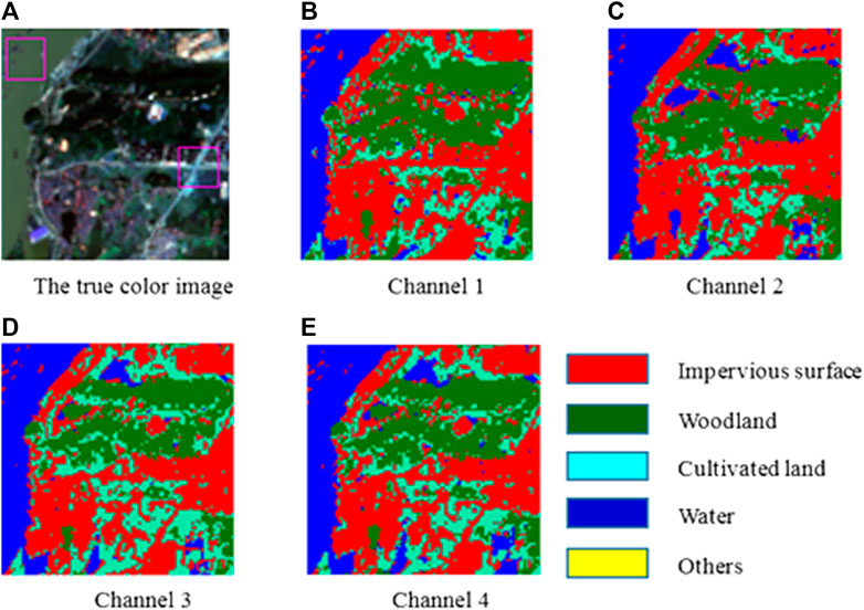
FIGURE 5. Results of the channel experiment. (A) The true color image. (B) Channel 1. (C) Channel 2. (D) Channel 3. (E) Channel 4.

FIGURE 6

FIGURE 6. Kappa coefficient and overall accuracy.

The confusion matrix is mainly used to describe the case in which features are incorrectly classified. The calculation of kappa coefficients is based on the confusion matrix, and the results are used for consistency checks. This paper calculates the kappa coefficient and confusion matrix based on 10 test datasets to assess the quality of the model. The confusion matrix of channel 4 is shown in Table 4. The confusion matrix indicates that the classification accuracy for the categories other than water areas is not very high. Notably, in some areas in Wuhan, such as the East Lake Moshan Scenic Area of Wuhan University, which has impervious surfaces, woodland and water, there are several mixed features; additionally, in the suburbs of Wuhan, there are impervious surfaces, cultivated land areas and water areas. The highest classification accuracy is obtained for water, and the correct classification rate is as high as 91.2%. In the confusion matrix, the classification accuracy of other types of land use is comparatively low, mainly because there are many mixed pixels in woodland and town areas, and it is difficult to eliminate this noise when channel 4 extracts features.

TABLE 4

TABLE 4. Channel 4 confusion matrix.

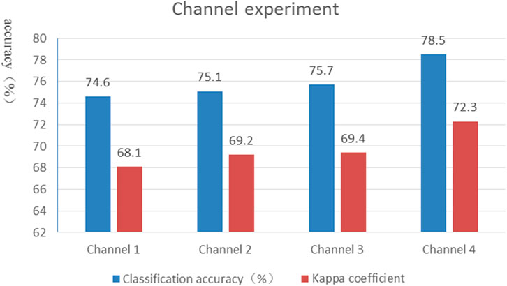
Figure 6 shows the overall classification accuracy for the four channels. Notably, the classification accuracy of the four channels is approximately 75%. Channel 4 displays the highest classification accuracy, and channel 2 and channel 3 exhibit similar classification accuracies. Additionally, using a multichannel input enhances feature extraction with the CNN, and the classification accuracy of the CNN is improved when the image is enhanced. Moreover, the kappa coefficient is stable at approximately 0.7, and accuracy is generally proportional to the kappa coefficient.

To explore the influence of neighborhood windows of different sizes on the classification accuracy, this paper selects four neighborhoods with sizes of 21 × 21, 15 × 15, 11 × 11, and 7 × 7 to conduct experiments; in these cases, the input data channel is channel 4. Figure 8 is a true-color image, and the resulting images with neighborhood windows of 21 × 21, 15 × 15, 11 × 11, and 7 × 7 are shown from left to right. As shown in Figure 7, the salt and pepper effect is most obvious for the 21 × 21 neighborhood window. There are small fragments in each category, such as in the red area in the middle of the image and in the green area in the upper right, and there are many category mixing problems at land type edges. The 11 × 11 neighborhood window and 7 × 7 neighborhood window yield similar classification effects. Additionally, the salt and pepper effect is alleviated to some extent. With these windows, the whole image is smoother than the images obtained with the 21 × 21 neighborhood window and 15 × 15 neighborhood window, but there are still small fragments present. From the perspective of model training, the 21 × 21 neighborhood window produces rich features, but redundant information is obtained, and there is considerable noise in the image, which affects the final classification results. Although the information obtained with the 7 × 7 neighborhood window is useful for assessing the pixel types, it is not conducive for constructing a deep model and cannot be applied to train complex datasets. The information obtained with the 11 × 11 neighborhood window can be passed to two pooling layers, and the classification effect is obviously better than that for the 15 × 15 and 21 × 21 neighborhood windows.

FIGURE 7

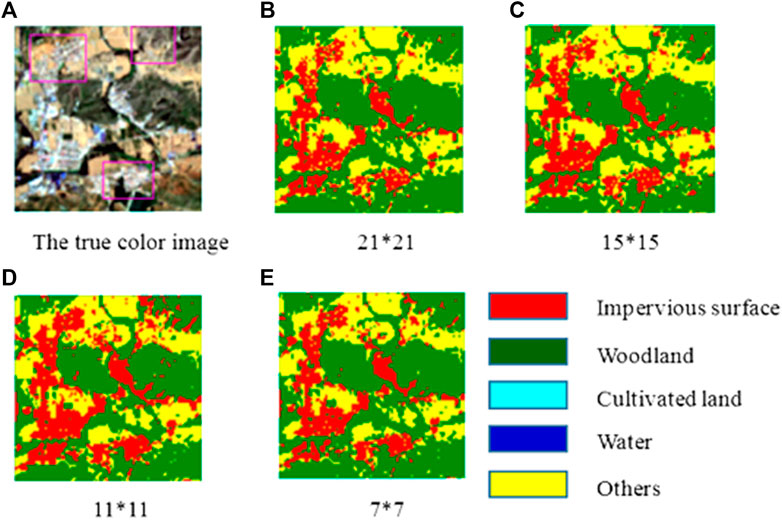
FIGURE 7. The comparison of different size of neighborhood window of image patch. (A) The true color image. (B) 21*21. (C) 15*15. (D) 11*11. (E) 7*7.

The confusion matrix for the 21 × 21 neighborhood window is shown in Table 5. In the four neighborhood window experiments, the classification of water areas is the best, but in some areas, such as farmland areas, water and cultivated land are easily confused. For water areas, woodlands and arable land, the surrounding pixels are generally associated with the same land use type, so small neighborhood windows can most accurately describe the category at the central point of the window. If the neighborhood window is too large, the classification accuracy will be low for these land types.

TABLE 5

TABLE 5. Confusion matrix for the 21 × 21 neighborhood window.

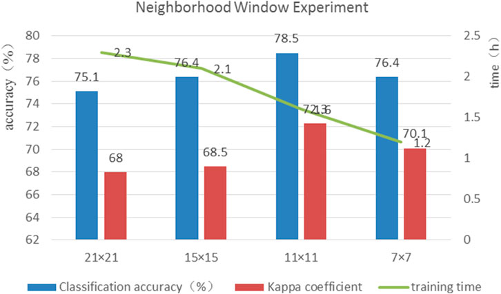
Figure 8 shows the kappa coefficients, classification accuracy and model training times for the four neighborhood windows. Appropriate neighborhood windows can effectively improve the classification accuracy. However, when the neighborhood window is reduced to 7 × 7, the classification accuracy does not increase significantly, and it is difficult to build a deep neural network model. In terms of training time, the 21 × 21 neighborhood window includes many pixels, thus requiring a large amount of memory and a long training time. The experimental results show that the training time of the model increases and the training accuracy decreases when the neighborhood window size is too large. Of the four neighborhood windows, the 11 × 11 neighborhood window yields the best classification effect and is most suitable for the input window of the model.

FIGURE 8

FIGURE 8. Kappa coefficient, overall accuracy and training time.

3.3 The results of the object-oriented convolutional neural network

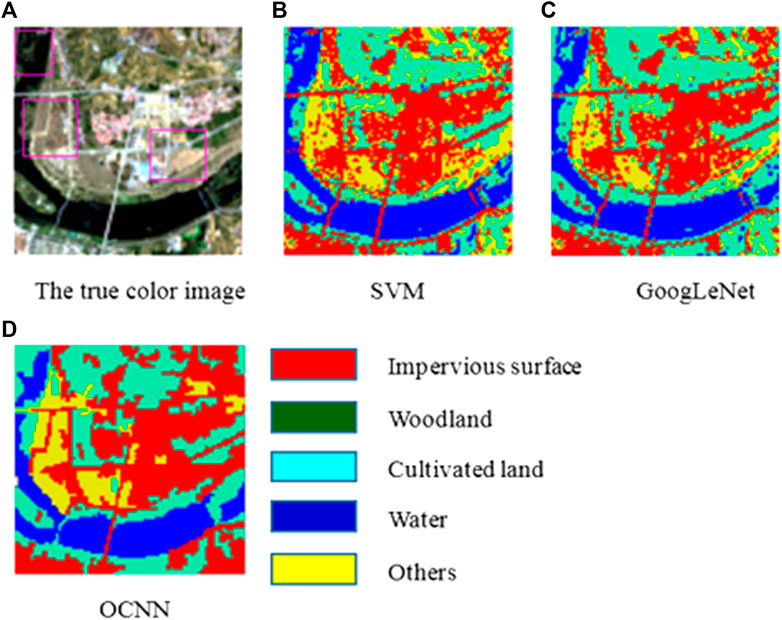
To verify the effectiveness of the combination of the object-oriented method and GoogLeNet, this paper used a support vector machine (SVM), GoogLeNet and object-oriented GoogLeNet to conduct comparative experiments. The original true color image and classification results are shown in Figure 9. In the SVM classification method, there are many fragmentation problems for the categories other than water, and the classification results are very poor at the junctions of multiple objects. The classification results of GoogLeNet are relatively good compared to those of the SVM, but they are not optimal. The object-oriented CNN (OCNN) eliminates salt and pepper effects to a certain extent and can effectively distinguish the boundaries of objects. The proposed method can notably increase the classification accuracy for the water, woodland and arable land classes.

FIGURE 9

FIGURE 9. Experimental results. (A) The true color image. (B) SVM. (C) GoogLeNet. (D) OCNN.

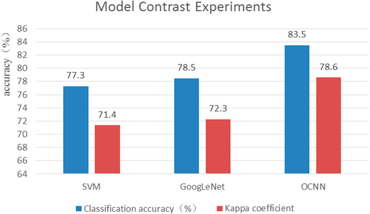
Figure 10 shows the classification accuracy in the three experiments. From the overall accuracy results, we can see that the classification accuracy of GoogLeNet is similar to that of the SVM. The accuracy of the OCNN is obviously higher than that of the other two methods. The classification accuracy for water areas is as high as 95%. The classification accuracy values for cultivated land and woodland areas are 7 and 4% higher, respectively, than those obtained with GoogLeNet. The classification accuracy for other categories is slightly lower at only 76%, while the SVM achieves an accuracy of 78% for these categories. This difference is mainly because 1/3 fewer training samples are available for these categories than for those above, and the updating of model parameters is not sufficient. The classification accuracy of the proposed method is 7 and 5% higher than the accuracy achieved with the SVM and traditional GoogLeNet, respectively. This finding indicates that the OCNN can effectively improve the classification accuracy.

FIGURE 10

FIGURE 10. The overall accuracy and kappa coefficients of the three classifiers.

4 Discussion and conclusion

The classification accuracy of the OCNN is 5% higher than that of the basic CNN. Moreover, the classification diagram of the experimental results indicates that the OCNN method successfully solves the salt and pepper problem and improves the classification accuracy. Other studies have also shown that object-oriented classification methods can solve salt and pepper issues. In vegetation classification and detailed land cover classification, researchers have noted that object-oriented methods are able to overcome the salt and pepper problem (Yu et al., 2006), (Pu et al., 2011).

Although our method has achieved good classification results, there are still areas that need to be improved, mainly reflected in the following aspects: 1) in object segmentation, only the segmentation scale parameters are considered. In the future, shape parameters and compactness parameters will be added to explore whether objects can be more accurately segmented. 2) the numbers of samples in the water, woodland and other categories were insufficient and will to be increased in the future. 3) the optimal window size needs to be obtained through a lot of experiments, we will add more experiments or study new methods to obtain the optimal value. 4) It is difficult to select parameters or network structure in the proposed method, especially the combination of different parameters and combination of different network structures. The orthogonal test methods used for parameter selection will be considered in the future, and an integrated OCNN will be combined with majority voting to improve the classification accuracy.

Data availability statement

The original contributions presented in the study are included in the article/supplementary material, further inquiries can be directed to the corresponding author.

Author contributions

Conceptualization, FL, LD, XC, and XG; methodology, FL and LD; 419 software, FL and XC; validation,LD, XC, and XG; formal analysis, FL and LD; investigation, 420 XC; resources, FL, LD, and XC; data curation, XC and XG; writing—original draft preparation, 421 LD and XG; writing—review and editing, FL and XC; visualization,FL and LD; supervision, 422 FL, LD and XC; project administration, LD; All authors have read and agreed to the published 423 version of the manuscript.

Conflict of interest

The authors declare that the research was conducted in the absence of any commercial or financial relationships that could be construed as a potential conflict of interest.

Publisher’s note

All claims expressed in this article are solely those of the authors and do not necessarily represent those of their affiliated organizations, or those of the publisher, the editors and the reviewers. Any product that may be evaluated in this article, or claim that may be made by its manufacturer, is not guaranteed or endorsed by the publisher.

References

Belward, A. S., and Hoyos, A. D. (1987). A comparison of supervised maximum likelihood and decision tree classification for crop cover estimation from multitemporal LANDSAT MSS data. Int. J. Remote Sens. 8 (2), 229–235. doi:10.1080/01431168708948636

CrossRef Full Text | Google Scholar

Blanzieri, E., and Melgani, F. (2008). Nearest neighbor classification of remote sensing images with the maximal margin principle. IEEE Trans. Geosci. Remote Sens. 46 (6), 1804–1811. doi:10.1109/tgrs.2008.916090

CrossRef Full Text | Google Scholar

Blaschke, T., Lang, S., Lorup, E., Strobl, J., and Zeil, P. (2000). Object-oriented image processing in an integrated GIS/remote sensing environment and perspectives for environmental applications[C] environmental information for planning. Politics & the Public.

Google Scholar

Camps-Valls, G., Gomez-Chova, L., Calpe-Maravilla, J., Soria-Olivas, E., and Moreno, J. (2003). Kernel methods for HyMap imagery knowledge discovery[J]. Proc. SPIE. Int. Soc. Opt. Eng., 5238. doi:10.1117/12.510719

CrossRef Full Text | Google Scholar

Chen, Y., Jiang, H., Li, C., Jia, X., and Ghamisi, P. (2016). Deep feature extraction and classification of hyperspectral images based on convolutional neural networks. IEEE Trans. Geosci. Remote Sens. 54 (10), 6232–6251. doi:10.1109/tgrs.2016.2584107

CrossRef Full Text | Google Scholar

Dang, Y., Zhang, J. X., Deng, K. Z., Zhao, Y., and Yu, F. (2017). Study on the evaluation of land cover classification using remote sensing images based on AlexNet. J. Geo-information Sci. 19 (11), 1530–1537.

Google Scholar

Foley, J. A., Defries, R., Asner, G. P., Barford, C., Bonan, G., Carpenter, S. R., et al. (2005). Global consequences of land use. Science 309 (5734), 570–574. doi:10.1126/science.1111772

PubMed Abstract | CrossRef Full Text | Google Scholar

Foody, G. M . (2002). Status of land cover classification accuracy assessment. Remote Sens. Environ. 80 (1), 185–201. doi:10.1016/s0034-4257(01)00295-4

CrossRef Full Text | Google Scholar

Glorot, X., Bordes, A., and Bengio, Y. (2010). “Deep sparse rectifier neural networks[C]//,” in Proceedings of the 14th International Conference on Artificial Intelligence and Statistics, Fort Lauderdale, FL, USA, 11-13 April 2011. AISTATS.

Google Scholar

Graves, A. (2008). Supervised sequence labelling with recurrent neural networks. Munich, Bavaria, Germany: Studies in Computational Intelligence, 385.

Google Scholar

Griffith, J . (1979). Remote sensing and image interpretation[M]. John Wiley & Sons.

Google Scholar

Gu, J., Wang, Z., Kuen, J., Ma, L., Shahroudy, A., Shuai, B., et al. (2015). Recent advances in convolutional neural networks. Pattern Recognit. DAGM. 77, 354–377. doi:10.1016/j.patcog.2017.10.013

CrossRef Full Text | Google Scholar

He, K., Zhang, X., Ren, S., and Sun, J. (2016). “Deep residual learning for image recognition,” in IEEE Conference on Computer Vision and Pattern Recognition.

CrossRef Full Text | Google Scholar

Hinton, G. E., and Salakhutdinov, R. R. (2006). Reducing the dimensionality of data with neural networks. Science 313, 504–507. doi:10.1126/science.1127647

PubMed Abstract | CrossRef Full Text | Google Scholar

Hong, H., Xu, C., Liu, X., and Chen, W. (2016). Interpretation and research on landuse based on Landsat 7 ETM plus remote sensing data. IOP Conf. Ser. Earth Environ. Sci. 44, 032003. doi:10.1088/1755-1315/44/3/032003

CrossRef Full Text | Google Scholar

Huang, Bo, Zhao, Bei, and Song, Yimeng (2018). Urban land-use mapping using a deep convolutional neural network with high spatial resolution multispectral remote sensing imagery. Remote Sens. Environ. 214, 73–86. doi:10.1016/j.rse.2018.04.050

CrossRef Full Text | Google Scholar

Huang, Zhi, and Jia, Xiuping (2012). Integrating remotely sensed data, GIS and expert knowledge to update object-based land use/land cover information. Int. J. Remote Sens. 33 (4), 905–921. doi:10.1080/01431161.2010.536182

CrossRef Full Text | Google Scholar

Jakubauskas, Mark E., Legates, David R., and JudeKastens, H. (2002). Crop identification using harmonic analysis of time-series AVHRR NDVI data. Comput. Electron. Agric. 37 (1), 127–139. doi:10.1016/s0168-1699(02)00116-3

CrossRef Full Text | Google Scholar

Krizhevsky, A., Sutskever, I., and Hinton, G. (2012). “Imagenet classification with deep convolutional neural networks,” in NIPS. Curran Associates Inc.

Google Scholar

L Turner, B., Lambin, E. F., and Reenberg, A. (2008). The emergence of land change science for global environmental change and sustainability. Proc. Natl. Acad. Sci. U. S. A. 104 (52), 20666–20671. doi:10.1073/pnas.0704119104

PubMed Abstract | CrossRef Full Text | Google Scholar

Lecun, Y., Bottou, L., Bengio, Y., and Haffner, P. (1998). Gradient-based learning applied to document recognition. Proc. IEEE 86 (11), 2278–2324. doi:10.1109/5.726791

CrossRef Full Text | Google Scholar

LeCun, Y., Boser, B., Denker, J. S., Henderson, D., Howard, R. E., Hubbard, W., et al. (1989). Backpropagation applied to handwritten zip code recognition. Neural Comput. 1 (4), 541–551. doi:10.1162/neco.1989.1.4.541

CrossRef Full Text | Google Scholar

Lee, D. S., Shan, J., and Bethel, J. S. (2003). Class-guided building extraction from ikonos imagery. Photogramm. Eng. remote Sens. 69 (2), 143–150. doi:10.14358/pers.69.2.143

CrossRef Full Text | Google Scholar

Li, Miao, Zang, Shuying, Zhang, Bing, Li, Shanshan, and Wu, Changshan (2014). A review of remote sensing image classification techniques: The role of spatio-contextual information. Eur. J. Remote Sens. 47 (1), 389–411. doi:10.5721/eujrs20144723

CrossRef Full Text | Google Scholar

Linda, S., Dmitry, S., Myroslava, L., Ian, M., Steffen, F., Alexis, C., et al. (2015). Building a hybrid land cover map with crowdsourcing and geographically weighted regression[J]. ISPRS J. Photogrammetry Remote Sens. 103, 48.

Google Scholar

Lu, D., and Weng, Q. (2007). A survey of image classification methods and techniques for improving classification performance. Int. J. Remote Sens. 28 (5), 823–870. doi:10.1080/01431160600746456

CrossRef Full Text | Google Scholar

Mash, R., Borghetti, B., and Pecarina, J. (2016). “Improved aircraft recognition for aerial refueling through data augmentation in convolutional neural networks.” in International Symposium on Visual Computing Springer International Publishing.

CrossRef Full Text | Google Scholar

Mather, P. M. (1985). A computationally-efficient maximum-likelihood classifier employing prior probabilities for remotely-sensed data. Int. J. Remote Sens. 6 (2), 369–376. doi:10.1080/01431168508948456

CrossRef Full Text | Google Scholar

McFEETERS, S. K. (1996). The use of the Normalized Difference Water Index (NDWI) in the delineation of open water features. Int. J. Remote Sens. 17 (7), 1425–1432. doi:10.1080/01431169608948714

CrossRef Full Text | Google Scholar

Murthy, C. S., Raju, P. V., and Badrinath, K. V. S. (2003). Classification of wheat crop with multi-temporal images: Performance of maximum likelihood and artificial neural networks. Int. J. Remote Sens. 24 (23), 4871–4890. doi:10.1080/0143116031000070490

CrossRef Full Text | Google Scholar

Nair, V., and Hinton, G. E. (2010). “Rectified linear units improve restricted Boltzmann machines,” in Proceedings of the 27th International Conference on Machine Learning, haifa,israel, June 21-24, 2010.

Google Scholar

Peng, Z., Xin, N., Yong, D., and Fei, X. (2016). “Airport detection from remote sensing images using transferable convolutional neural networks[C],” in International joint conference on neural networks, Vancouver, BC, Canada, 24-29 July 2016 (IEEE).

Google Scholar

Pu, R., Landry, S., and Yu, Q. (2011). Object-based urban detailed land cover classification with high spatial resolution IKONOS imagery. Int. J. Remote Sens. 32 (12), 3285–3308. doi:10.1080/01431161003745657

CrossRef Full Text | Google Scholar

Puletti, Nicola, Perria, Rita, and Storchi, Paolo (2014). Unsupervised classification of very high remotely sensed images for grapevine rows detection. Eur. J. Remote Sens. 47, 45–54. doi:10.5721/eujrs20144704

CrossRef Full Text | Google Scholar

Rogan, John, and Chen, DongMei (2004). Remote sensing technology for mapping and monitoring land-cover and land-use change. Prog. Plan. 61 (4), 301–325. doi:10.1016/s0305-9006(03)00066-7

CrossRef Full Text | Google Scholar

Rumelhart, D. E., Hinton, G. E., and Williams, R. J. (1986). Learning representations by back-propagating errors. Nature 323 (9), 533–536. doi:10.1038/323533a0

CrossRef Full Text | Google Scholar

Sekovski, I., Stecchi, F., Mancini, F., and Del Rio, L. (2014). Image classification methods applied to shoreline extraction on very high-resolution multispectral imagery. Int. J. Remote Sens. 35 (10), 3556–3578. doi:10.1080/01431161.2014.907939

CrossRef Full Text | Google Scholar

Simonyan, K., and Zisserman, A. (2014). “Very deep convolutional networks for large-scale image recognition,” in International Conference of Learning Representation.

Google Scholar

Sterling, S. M., Ducharne, A., and Polcher, J. (2012). The impact of global land-cover change on the terrestrial water cycle. Nat. Clim. Chang. 3 (4), 385–390. doi:10.1038/nclimate1690

CrossRef Full Text | Google Scholar

Su, W., Li, J., Chen, Y., Liu, Z., Zhang, J., Low, T. M., et al. (2008). Textural and local spatial statistics for the object‐oriented classification of urban areas using high resolution imagery. Int. J. Remote Sens. 29 (11), 3105–3117. doi:10.1080/01431160701469016

CrossRef Full Text | Google Scholar

Sun, Z. P., Shen, W. M., Wei, B., Liu, X., Su, W., Zhang, C., et al. (2010). Object-oriented land cover classification using HJ-1 remote sensing imagery. Sci. China Earth Sci. 53 (1), 34–44. doi:10.1007/s11430-010-4133-6

CrossRef Full Text | Google Scholar

Szegedy, C., Liu, N. W., Jia, N. Y., Sermanet, P., and Rabinovich, A. (2015). “Going deeper with convolutions,” in IEEE Conference on Computer Vision and Pattern Recognition (CVPR) IEEE Computer Society, Boston, MA, USA, 7-12 June 2015.

CrossRef Full Text | Google Scholar

Wang, H., Wang, Y., Zhang, Q., Xiang, S., and Pan, C. (2017). Gated convolutional neural network for semantic segmentation in high-resolution images. REMOTE Sens. 9 (5), 446. doi:10.3390/rs9050446

CrossRef Full Text | Google Scholar

Wei, H., Yangyu, H., Li, W., Fan, Z., and Hengchao, L. (2015). Deep convolutional neural networks for hyperspectral image classification[J]. J. Sensors 2015, 1–12. doi:10.1155/2015/258619

CrossRef Full Text | Google Scholar

Wei, J., Guojin, H., Tengfei, L., Yuan, N., Liu, H., Peng, Y., et al. (2018). Multilayer perceptron neural network for surface water extraction in Landsat 8 OLI satellite images[J]. Remote Sens. 10 (5), 755. doi:10.3390/rs10050755

CrossRef Full Text | Google Scholar

Xu, Y., Xie, Z., Feng, Y. X., and Chen, Z. (2018). Road extraction from high-resolution remote sensing imagery using deep learning. REMOTE Sens. 10 (9), 1461. doi:10.3390/rs10091461

CrossRef Full Text | Google Scholar

Yang, Bo, Zeng, Faming, Yuan, Minghuan, Li, Deping, Qiu, Yonghong, and Li, Jingbao (2011). Measurement of dongting lake area based on visual interpretation of polders. Procedia Environ. Sci. 10, 2684–2689. doi:10.1016/j.proenv.2011.09.417

CrossRef Full Text | Google Scholar

Yang, C., Ying-Ying, C., and Yi, L. (2008). Object-oriented classification of remote sensing data for change detection. Jinan City, Shandong Province: Journal of Shandong Jianzhu University.

Google Scholar

Yang, D., and Du, X. (2017). An enhanced water index in extracting water bodies from Landsat TM imagery. Ann. GIS 23 (3), 141–148. doi:10.1080/19475683.2017.1340339

CrossRef Full Text | Google Scholar

Yang, H., Wu, P., Yao, X., Wu, Y., Wang, B., and Xu, Y. (2018). Building extraction in very high resolution imagery by dense-attention networks. REMOTE Sens. 10 (11), 1768. doi:10.3390/rs10111768

CrossRef Full Text | Google Scholar

Yu, Q., Gong, P., Clinton, N., Biging, G., Kelly, M., and Schirokauer, D. (2006). Object-based detailed vegetation classification with airborne high spatial resolution remote sensing imagery. Photogramm. Eng. remote Sens. 72 (7), 799–811. doi:10.14358/pers.72.7.799

CrossRef Full Text | Google Scholar

Yu, Shiqi, Jia, Sen, and Xu, Chunyan (2017). Convolutional neural networks for hyperspectral image classification[J]. Neurocomputing 219, 88. doi:10.1016/j.neucom.2016.09.010

CrossRef Full Text | Google Scholar

Zeiler, M. D., and Fergus, R. (2013). Stochastic pooling for regularization of deep convolutional neural networks[J]. Eprint Arxiv.

Google Scholar

Zha, Y., Gao, J., and Ni, S. (2003). Use of normalized difference built-up index in automatically mapping urban areas from TM imagery. Int. J. Remote Sens. 24 (3), 583–594. doi:10.1080/01431160304987

CrossRef Full Text | Google Scholar

Zhang, Ce, Pan, Xin, Li, Huapeng, Gardiner, Andy, Sargent, Isabel, Hare, Jonathon, et al. (2018). A hybrid MLP-CNN classifier for very fine resolution remotely sensed image classification. ISPRS J. Photogrammetry Remote Sens. 140, 133–144. doi:10.1016/j.isprsjprs.2017.07.014

CrossRef Full Text | Google Scholar

Zhang, C., Sargent, I., Pan, X., Li, H., Gardiner, A., Hare, J., et al. (2018). An object-based convolutional neural network (OCNN) for urban land use classification. Remote Sens. Environ. 216, 57. doi:10.1016/j.rse.2018.06.034

CrossRef Full Text | Google Scholar

Zhao, S., Liu, Y., Jie, J., Cheng, W., and Ruan, R. (2014). “Extraction of mangrove in Hainan Dongzhai Harbor based on CART decision tree[C]//,” in International Conference on Geoinformatics, Kaohsiung, 25-27 June 2014.

Google Scholar

Zheng, L., and Huang, W. (2015). Parameter optimization in multi-scale segmentation of high resolution remotely sensed image and its application in object-oriented classification. J. Subtropical Resour. Environ. 10 (4), 77–85. doi:10.2991/eers-15.2015.21

CrossRef Full Text | Google Scholar

Zhihong, G., and Xingwan, L. (2014). “Support vector machine and object-oriented classification for urban impervious surface extraction from satellite imagery[C]//,” in International Conference on Agro-geoinformatics, Beijing, China, 11-14 August 2014. IEEE.

Google Scholar