Reliability analysis of ground movement in tunnelling in spatially variable soil using equivalent parameters

The evaluation of the ground movement induced by tunnelling is of vital importance for the tunnel construction and the safety of the adjacent facilities. As the spatial variability of soil was widely acknowledged, more and more researches take insight into the uncertainty analysis for tunnelling. However, reliability analysis considering the spatial variability of soil is still a tough task since the accurate failure probability generally needs time-consuming calculation of random finite element/difference. Instead of conducting the direct Monte-Carlo simulation, this study utilizes a simplified framework to analyze the reliability of the ground movement of tunnelling. The main concept of this framework is adopting random variable model with equivalent parameters by producing the comparable failure probability as the results of random field model. Coupling with the variance reduction technique, the reliability analysis of tunnel ground movement considering more than one spatial variable can be addressed. Two tunnel cases are studied to explain the adaptability and accuracy of this simplified framework in tunnelling. The characteristic of the spatially variable soil is thoroughly comprehended through various parametric study, based on the robustness of the simplified framework. Results show that the simplified framework precisely predicts the tunnel reliability considering spatially variability of soil in a relatively efficient manner.

Introduction

Ground movement due to tunnelling is of great importance when assessing the risk of tunnel construction and adjacent existing structures, especially in urban areas. As a result, plenty of researches pay attention to this topic during past decades (Peck, 1969; Loganathan and Poulos, 1998; Zhang et al., 2011; Cui et al., 2021a; Cui et al., 2021b; Dong et al., 2022). When the soil assumed isotropic and homogeneous, these studies can be defined as deterministic analysis. These deterministic analyses give engineers plenty of experiences and convenient ways to evaluate the risk brought by tunnelling. However, soil shows strongly spatial variability due to the complex natural formation process and the artificial disturbance. As a major sources of uncertainty in geotechnical applications, the necessity of considering spatial variability (Phoon and Kulhawy, 1999; Dasaka and Zhang, 2012; Javankhoshdel et al., 2017) has been demonstrated in recent decades. Cami et al. (2020; 2021) provided a database table of horizontal and vertical scale of fluctuation values in different locations and for different materials, collected from published case studies, showing the spatial variability of soil from different areas. In addition, more typical value reflecting the spatial variability of soil can be referred to Stuedlein (2021). To further cope with the uncertainty, two different approaches are introduced.

The first is random variable method. In this method, the soil properties are assumed perfectly correlated, and each of them modeled through a single random variable. Due to the concise concept and simplicity, the random variable method has been widely used in estimating the face stability and ground movement of tunnelling (Mollon et al., 2012, 2013; Eshraghi and Zare, 2015; Miro et al., 2015). Based on kinematic theorem of limit analysis, the reliability of the tunnel face stability can be quickly displayed. By contrast, as the ground movement of tunnelling is a highly nonlinear problem controlled by multiple influencing parameters, most of the relevant researches (Lee et al., 1990; Migliazza et al., 2009; Chakeri et al., 2013) are conducted based on finite/finite difference method. However, the random variable method cannot actually reflect the soil spatial variability. To reproduce the spatial correlation of the soil property, another method is developed named random field method. According to the random field theory, researchers investigate a variety of geotechnical issues such as the bearing capacity of footings (Griffiths et al., 2006; Tabarroki et al., 2022a, 2022b), the stability of the slopes (Li et al., 2015; Huang and Leung, 2021), the basal-heave failure in braced excavation (Luo et al., 2012), the face stability of tunnels (Pan and Dias, 2017; Cheng et al., 2019a) and the ground movement induced by tunnelling (Cheng et al., 2019b).

Since the random variable method is lack of accounting for the spatial correlation, the random variable method is reported estimating the unrealistic estimation of reliability (Griffiths and Fenton, 2004; Griffiths et al., 2009; Wang et al., 2010). In general, deformation or even failure of soil in tunnelling will develop along the weak surface, which is similar to the slip surface in slope stability problem. The characteristics of soil parameters are weaker along the most critical path and thus the stress and displacement will pass through this critical path. For example, the mean and standard deviation of s_u (undrain shear strength) along the slip surface of slope are smaller than those of the whole field (Ching et al., 2014). However, this difference does not exist in random variable method. Owing to the perfect correlation assumption, the random variable method tends to result in a fixed deformation pattern, and thus cannot seek out the most critical path through the soil. This leads to unrealistic results when using the random variable method.

The random finite element/difference method (RFEM/RFDM) is generally utilized to solve out a complex geotechnical problem considering the spatial variability of soil. It combines the random field theory and finite element/difference method in the framework of Monte Carlo simulation (MCS). However, this method commonly requires for high cost and time-consuming calculation, especially when the probability of failure (P_f) is small. Cheng et al. (2019b) take relatively few simulations (i.e., 500 MCS) to represent the whole MCS to investigate the influence of spatial variability of soil on ground movement of tunnelling. Valuable conclusions have been drawn in his research such as the regulation of distribution and magnitude of ground movement in spatial variable soil. Nevertheless, as for the P_f, the analysis in this research may not be suitable for low probability problem, because of the inadequate times of MCS and the unrealistic values for correlation length. In his research, the P_f varies apparently with the correlation length in relatively large value (i.e., ≥60 m), but seldomly changes when the correlation length varies from 1 to 12 m. Nevertheless, the values (i.e., θ_x = θ_y ≥ 60 m) are out of the typical statistics for a wide range of spatially variable soils investigated by Phoon and Kulhawy (1999). Obviously, the conclusion for P_f according to Cheng et al. (2019b) has limitations when applied in practice. To overcome this problem, exploring efficient reliability analysis approaches becomes a trend in geotechnical reliability analysis (Wang et al., 2010; Jiang et al., 2014; Jiang et al., 2015; Li et al., 2016). To at least the author’s knowledge, these efficient methods are widely used in analyzing the slope stability or tunnel face stability problem, but few researches report these methods in reliability analysis of the ground movement induced by tunnelling.

Aiming at obtaining an accurate P_f for ground movement of tunnelling in spatial variable soil, this study presents a more reasonable and efficient reliability analysis through equivalent parameters. This efficient reliability analysis takes advantage of the simplified framework (Liu et al., 2018) which is first proposed to solving the slope stability problem. Based on the random field model, the regression method and MCS, this simplified framework will be introduced in detail in the following text. Through this simplified framework, the statistics of the equivalent parameters can be obtained. Using the regression method, the explicit response surface function of the random variable model is built. By inputting the statistics of equivalent parameters in the explicit response surface function of the random variable model, the cost for reliability analysis considering spatial variability is trimmed down. Reliability analysis is conducted on both a single spatial variable case and a multiple spatial variables case. The results verify the practical applicability of the simplified framework using equivalent parameters.

Development of the simplified framework

The simplified framework for reliability analysis using the equivalent parameters is firstly introduced by Li et al. (2017) and further extended by Liu et al. (2018). The main idea of this simplified framework is to find the equivalent parameters for the random variable model (RVM) based on the requirement that can provide comparable P_f value with the random field model (RFM). The corresponding RFM can reflect the spatial variability of the soil. Through the equivalence between the RFM and the RVM, the reliability approaches used in random variable method such as first-order reliability method and response surface method can be applied, and thus improves the computation efficiency of the reliability analysis considering spatial variability of the soil.

To be specific, in slope stability analysis, the equivalent parameters are defined as the parameters that enable the safety factor of RVM equals to that of RFM. In this study, for the ground movement of tunnelling, the equivalent parameters are defined as the parameters those enable the maximum of the ground settlement (S_max) of RVM and RFM to be the same. As the deformation pattern may be different in the RVM and RFM, these two models are not fully equivalent. However, the equivalence between RVM and RFM here is reasonably acceptable because this study focuses on the failure probability that only depends on the values of S_max, rather than the risk assessment affected by the deformation pattern. The included techniques in the framework will be introduced in detail in the following sections.

Establish the RFM

Several random field generation methods can be utilized, such as the midpoint method (Kiureghian and Ke, 1988), the local average subdivision (LAS) method (Vanmarcke, 2010), the shape function method (Liu et al., 1986)and the Karhunen–Loève (KL) expansion (Phoon et al., 2002). Due to the efficiency and accuracy of the KL expansion, it is adopted in this study. The KL expansion is introduced briefly in the following.

A random field H (A,θ) is a collection of random variables associated with a continuous index $A\in \Omega$, where Ω is an open set of Rⁿ describing the system geometry and $\theta \in \Theta$ is the coordinate in the outcome space. When discretizing a random field H (A,θ) using the KL expansion, the spectral decomposition of its autocorrelation function ρ (A₁, A₂) is conducted. The autocorrelation function is bounded, symmetric and positive definite. Hence, the discretization of a random field is defined by the eigenvalue problem of the homogenous Fredholm integral equation as:

$\underset{\mathrm{\Omega }}{{\displaystyle \int }}\rho \left(A_1,A_2\right)f_i\left(A_2\right)={\lambda }_i{f}_i\left(A_1\right)(1)$

where A₁ and A₂ represent the coordinates of two points in Ω; ρ(A₁, A₂) is value of the correlation function; λ_i and f_i (·) are the eigenvalues and eigenfunctions corresponding to ρ(A₁,A₂). For a two-dimensional (2-D) tunnel domain, A₁, A₂ can be denoted as (x₁, y₁) and (x₂, y₂). In this study, the Gaussian correlation function is chosen for representing the spatial variability of soil and is written as:

$\rho \left({\tau }_x,{\tau }_y\right)=\exp \left\{-\pi \left[{\left(\frac{{\tau }_x}{{\theta }_x}\right)}^2+{\left(\frac{{\tau }_y}{{\theta }_y}\right)}^2\right]\right\},(2)$

Where τ_x=|x₁-x₂|_, τ_y=|y₁-y₂| are the absolute distances between two points in the horizontal and vertical directions, respectively; and θ_x and θ_y are the horizontal and vertical correlation length, respectively. The detailed solution for the eigenvalue problem can be referred to Phoon et al. (2002). The series expansion of a 2-D random field H (x, y, θ) is expressed as:

$H\left(x,y,\theta \right)=\mu +{\displaystyle \sum }_{i=1}^{\infty }\sigma \sqrt{{\lambda }_i}{f}_i\left(x,y\right){\xi }_i\left(\theta \right)\left(x,y\in \mathrm{\Omega }\right),(3)$

where ξ_i(θ) is a set of orthogonal random coefficients (uncorrelated random variables with zero mean and unit variance); (x, y) represents the coordinate in the random field; μ and σ denote the mean and standard deviation of the random field. The approximate random field is defined by truncating the ordered series given in Eq. 3.

$\stackrel{\sim }{H}\left(x,y,\theta \right)=\mu +{\displaystyle \sum }_{i=1}^M\sigma \sqrt{{\lambda }_i}{f}_i\left(x,y\right){\xi }_i\left(\theta \right)\left(x,y\in \mathrm{\Omega }\right)(4)$

The value of M to be chosen strongly depends on the desired accuracy and the autocorrelation function of the random field.

Evaluation of the equivalent parameters

The basic precondition for obtaining the equivalent parameters is that RVM with the equivalent parameters produces a comparable failure probability as that calculated using the RFM with the original spatially variable parameters. In this study, the RVM is based on a numerical model which will be introduced in detail in Example I: A tunnel considering single spatially variable parameter and Example II: A tunnel considering multiple spatially variable parameters (seeing Figures 2, 10). Furthermore, the numerical model for the RVM is consistent with the RFM. Based on the establishment of the RFM and RVM, the equivalent parameters can be deduced by back-calculation from the RVM for a given Smax value collected from the existing RFM. According to Li et al. (2017), the evaluation of the equivalent parameters is achieved by trial-and-error method. This means that, when reproducing a result of the RFM, more than one times of RVM may be realized. This is time-consuming. Moreover, it is only applicable when a single spatial variable parameter is considered. To improve the efficiency, the evaluation of the equivalent parameters is incorporated with the explicit response surface function of the RVM (denoted ERVM hereafter) proposed by Liu et al. (2018).

The ERVM uses the explicit equations to substitute the original RVM. Without the process of trial-and-error, the ERVM can output the results quickly through algebraic operation. The establishment of the ERVM is introduced below. The ERVM is established based on the regression analysis of dataset (X, S_max) obtained from a variety of deterministic analysis, where X is a matrix with a dimension of N_t × n, and n is the number of the spatial variable soil parameters which are considered. Specifically, n =1 means only one spatial variable soil parameter is analyzed, and n =2 means two spatial variable soil parameters are analyzed. For a given S_max value obtained in advance from the RFM, the equivalent parameters can be easily obtained through the ERVM. Then the statistics such as means, standard deviation and probability density function can be determined.

The back-calculation will be successfully conducted when n =1. However, when n>1, the solution will be nonunique. To cope with this problem, the following strategy is used in this study:

1) Determine a soil parameter to be back-calculated for a given S_max.

2) Perform the variance reduction technique on the remaining n−1 soil parameters.

3) Randomly generate n−1 random variable samples according to the statistics obtained in Step (2) and substitute the sample values into the ERVM together with the given S_max to back-calculate the equivalent value of the soil parameter that is pre-specified in Step (1). It means that only one type of equivalent parameter is required to be back-calculated for a given equivalent S_max.

Process of the simplified framework

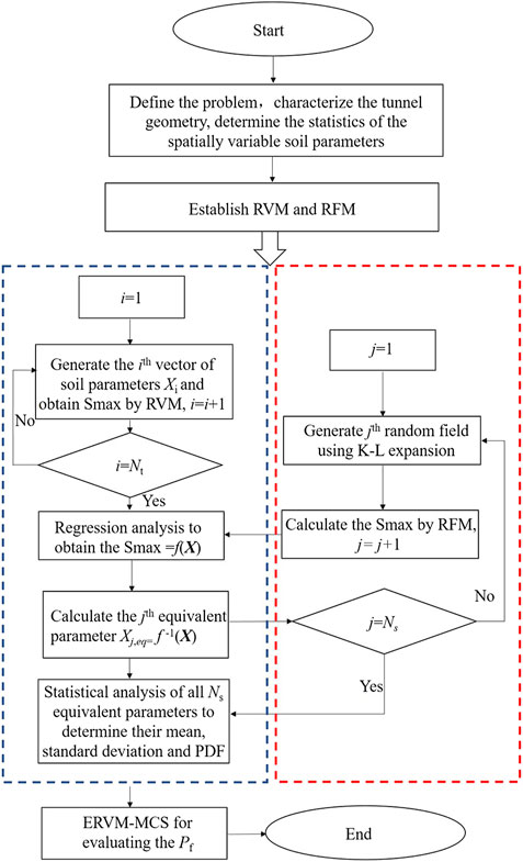
To further facilitate the understanding and application of the simplified framework, Figure 1 schematically shows the flowchart of the proposed reliability analysis process. In general, the flowchart mainly consists of five steps, which are shown as follows:

1) Collect the required data of geotechnical and geometrical parameters for reliability analysis of tunnel ground movement, including but not limited to shear strength, unit weight, tunnel diameter and tunnel axis depth. Then, select the stochastic parameters and characterize their statistics, including the means, coefficients of the variation (COVs), probability density functions (PDFs), auto correlation functions (ACFs), and correlation length (θ).

2) Establish RVM with the known information of the geotechnical and geometrical parameters obtained in Step (1). Perform N_t realizations of RVM and obtain the relationship between S_max and X by regression analysis. Develop the ERVM, i.e., S_max = f(X).

3) Generate the random field based on KL expansion and establish RFM with the known information of the geotechnical and geometrical parameters obtained in Step (1). Perform N_s realizations of RFM to form the samples to obtain the equivalent parameters.

4) The samples for S_max obtained in Step (3) are then substituted into ERVM in Step (2) for back-calculating the equivalent parameters values (i.e., X = f⁻¹(S_max)). A statistical analysis is then conducted to obtain the means, COVs and PDFs of the equivalent parameters. When more than one soil parameters are assumed spatially correlated, the strategy including the variance reduction technique introduced in Evaluation of the equivalent parameters should be used.

5) Conduct the reliability analysis based on MCS (or other reliability approaches used in random variable method) in ERVM with the statistics of the equivalent parameters obtained in Step (4).

FIGURE 1

FIGURE 1. Flowchart for the simplified framework for reliability analysis.

Example I: A tunnel considering single spatially variable parameter

Establish the RVM and RFM

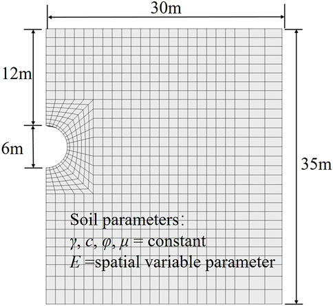
The simplified framework is first applied to a tunnel of which the stochastic ground movement is only controlled by the young’s modulus E. Owing to symmetry, half of the tunnel domain is considered in this study. Figure 2 shows the typical mesh and model domain of the numerical model. The numerical model is modeled by 1754 element zones and 2,784 grid points. To maintain the calculation efficiency, the mesh is finer around the tunnel and becomes sparse away from the tunnel. As shown in this figure, the tunnel crown depth is 12 m and the tunnel diameter is 6 m. The constitutive model of the soil is Mohr-Coulomb model. The unit weight of the soil γ is 18 kN/m³. The friction angle φ and the cohesion c of the soil is 8.5° and 13 kPa respectively. The Poisson’s ratio of the soil is 0.3. To cope with the spatial variability of E, the random field is generated by KL expansion as introduced in Establish the RFM. E is assumed to be subjected to the lognormal stationary random field with a mean μ_E of 12 MPa. The coefficient of variation COV_E is 0.3. Both the horizontal and vertical correlation length θ_x and θ_y are 60 m. The stress release method is adopted and the stress release ratio is set 0.1 in both RVM and RFM. The constitutive model of the lining segments is elastic model. The unit weight of the lining segments is 24 kN/m³. The thickness of the lining segments is 0.3 m. The Poisson’s ratio of the lining segments is 0.2. The young’s modulus of the lining segments is 15 GPa. It should be noted that this numerical model as well as the value of the relevant parameters are basically obtained according to Cheng et al. (2019b), therefore the results can be compared with Cheng et al. (2019b) for verification of the simplified framework.

FIGURE 2

FIGURE 2. Typical mesh and model domain for example I.

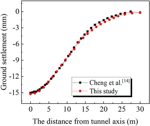
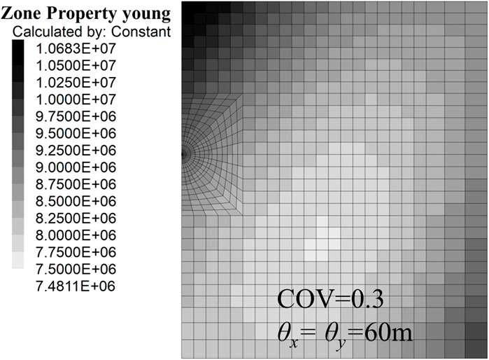
Figure 3 shows a certain realization of RVM which provides an S_max of 15 mm when inputting E as a spatial constant with a value of μ_E. The ground settlement profile is highly consistent with the result reported by Cheng et al. (2019b). This indicates the accuracy of the numerical model, thereby ensuring its applicability of the subsequent analysis. This numerical model is further used in establishing the RFM. Figure 4 illustrates certain realization of RFM, in which dark color indicates large E, whereas light color represents small E.

FIGURE 3

FIGURE 3. The verification of the numerical model.

FIGURE 4

FIGURE 4. Certain realization of RFM based on isotropic random field.

Determination of the equivalent parameters

In this section, the equivalent young’s modulus E_eq is determined. According to the flowchart depicted in Figure 1, the first step is to establish the ERVM for the ground movement of tunnelling through a certain number of realizations of RVM. Thus, 15 samples of E selected from the range of (μ_E − 3σ_E, μ_E + 3σ_E) are input in the RVM for establishing the ERVM. Figure 5A plots the results of the 15 realizations simulations of RVM. A linear relationship between S_max and 1/E can be observed according to the scatter points in Figure 5A. This fits the practice because when infinite E is adopted, the deformation of soil will tend to be 0. By conducting the linear regression analysis, the explicit response surface function of the RVM can be deduced as:

$S_{\max }\left(E\right)=169/E(5)$

FIGURE 5

FIGURE 5. Dataset and verification for the ERVM.

One-hundred realizations of RVM where the value of E is randomly generated according to the PDF of it are utilized to verify the accuracy of the ERVM. Figure 5B illustrates the comparison between the S_max predicted by Eq. 5 and obtained from the 100 realizations of RVM. The S_max from the RVM and ERVM agree well with each other, indicating that the ERVM can be effectively applied to back-calculate the equivalent parameters.

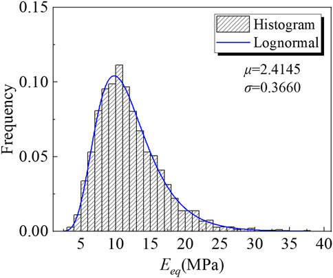
Next, following the flowchart in Figure 1, N_s realizations of RFM should be generated for estimating the statistics of E_eq. The S_max obtained through N_s realizations of RFM is back-calculated in Eq. 5 to form the dataset for E_eq. By performing the statistical analysis, the mean μ_Eeq, the standard deviation σ_Eeq and the PDF of the E_eq can be deduced based on the dataset of E_eq. To form the dataset for E_eq, the realizations times N_s should be determined in advance. The determination of the value of N_s is vital, because the accuracy increases with N_s, whereas the computational efficiency decreases with N_s. Therefore, a reasonable value is determined according to a sensitivity study in which the variation of the statistics of E_eq with N_s is analyzed. Figure 6 plots the variations of the μ_Eeq and σ_Eeq with N_s. As shown in both figures, the statistics varies greatly when N_s is lower than 3,000, but this becomes insignificantly when N_s exceeds 3,000. As a result, N_s is determined as 3,000 in this section. Figure 7 shows the probability histogram of the E_eq. As shown in Figure 7, the probability histogram is well fit by the lognormal distribution and the goodness of fit is 0.99. μ_Eeq and σ_Eeq of this lognormal distribution is 11.18mm and 0.366. The reliability analysis is processed based on these statistics incorporated with Eq. 5.

FIGURE 6

FIGURE 6. Variation of μ_Eeq and σ_Eeq with N_s.

FIGURE 7

FIGURE 7. The probability histogram of E_eq.

Reliability analysis

When calculating P_f corresponding to the maximum of the ground surface settlement, the performance function is expressed as:

$G=S_{\max }-s,(6)$

where s is the allowable S_max. In this study, s=20 mm. For simplicity, several abbreviations such as MCS, EQP+MCS and EQP+ERVM +MCS are introduced to better compare the results from different methods. It should be noted that the EQP represents the equivalent parameter and in this section is E_eq. MCS denotes the direct Monte-Carlo Simulation based on the random field model shown in Figure 4; EQP+MCS is the direct Monte-Carlo Simulations based on the random variable model using the equivalent parameters introduced in last section; EQP+ERVM+MCS represents the Monte-Carlo Simulations based on the explicit response surface function of the random variable model using the equivalent parameters, namely the simplified framework. To be specific, the numerical model used in both random field model and random variable model is the same with which has been introduced in Establish the RVM and RFM (i.e., Figure 2). The explicit response surface function of the random variable model can be referred to Eq. 5. In addition, the number in the bracket represents the realization times of MCS in each method and this number is set 10,000 in all three methods mentioned above. The P_f estimated by the EQP+ERVM+MCS is 0.2274. This value is consistent with the result of the MCS which is 0.2269, showing that the simplified framework with the statistics of E_eq can accurately reflect the spatial variability of the soil. Moreover, this result also matches well with the results by the EQP+MCS (P_f = 0.2203), further verifying the accuracy of the ERVM (i.e., Eq. 5). When compared to Cheng et al. (2019b) (P_f = 0.2045), the EQP+ERVM+MCS provides a larger value of P_f. However, the error between these two methods is acceptable for two reasons. First, the P_f estimated in Cheng et al. (2019b) is relatively rough as only 500 realizations MCS were conducted. Second, as reported in previous study (Li et al., 2015), the Gaussian correlation function used in this study may result in larger estimations of the P_f than other correlation functions.

In the previous study (Cheng et al., 2019a), the relationship between P_f and s (the allowable S_max) was presented. These results are also used in this study for comparison. Figure 8 compares the P_f derived from the simplified framework, MCS (500) and Cheng et al. (2019a). Figures 8A,B show the variation of P_f when s ranges in 10–35mm and 35–55 mm respectively. It should be noted that, according to Cheng et al. (2019a), P_f approaches 0 as the s exceeds 30 mm and thus the corresponding results are not to be found. Therefore, the results of 500 times of direct MCS based on RFM are shown instead in Figure 8. As plotted in Figure 8A, the three methods showing good consistency with each other implying the good performance of the proposed simplified framework. However, P_f decreases greatly when s grows and deviations are observed between EQP+ERVM+MCS and MCS (500) (seeing Figure 8B). As can be seen in Figure 8B, the MCS (500) shows big disadvantages in estimating P_f. Discontinuity in P_f estimated by the MCS (500) is observed when s grows. When s is in the range of 35–41 mm, 43–45 mm or 48–50 mm, P_f stays constant. On the contrary, sharply change is observed when s is in the range of 41–43 mm, 45–48 mm or 50–52 mm. This greatly deviates from the practice. Even if this is a low probability problem, the inaccurate P_f may produce great risk as the loss is relatively large. In contrast, P_f decreases more continuously with s when using the proposed simplified framework. As a result, MCS (500) is only adequate for a reasonable P_f at a high probability level whereas the proposed simplified framework shows good performance in both high and low probability level. Overall, the accuracy as well as the improvement of the simplified framework has been verified.

FIGURE 8

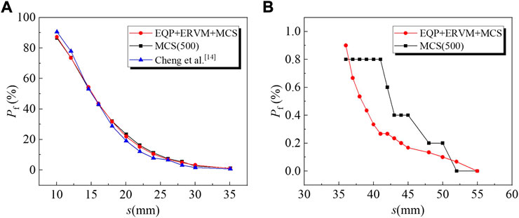
FIGURE 8. Comparison between the simplified framework, MCS (500) and Cheng et al. (2019a).

Parametric study

The effect of the spatial variability on the reliability analysis results is testified utilizing the simplified framework. Several parameters are investigated such as the horizontal and vertical correlation distances (i.e., θ_x and θ_y) and the coefficient of variation COV. The results of the direct MCS (500, 10,000) are also presented in this section to explain the accuracy and improvement of the simplified framework. Different from the isotropic random field generated in Cheng et al. (2019b), the anisotropic random field is generated with more reasonable θ_x and θ_y values by referring to the typical statistics for a wide range of spatially variable soils (Phoon and Kulhawy, 1999). θ_x varies from 10 to 40 m with an interval of 10m, whereas θ_y varies from 0.5 to 3.0 m with an interval of 0.5 m. In addition, COV ranges from 0.1 to 0.5 with an interval of 0.1. Only one parameter is changed in the parametric study and the remaining parameters is equal to the basic case of which θ_x=20m, θ_y=2.0 m and COV=0.3.

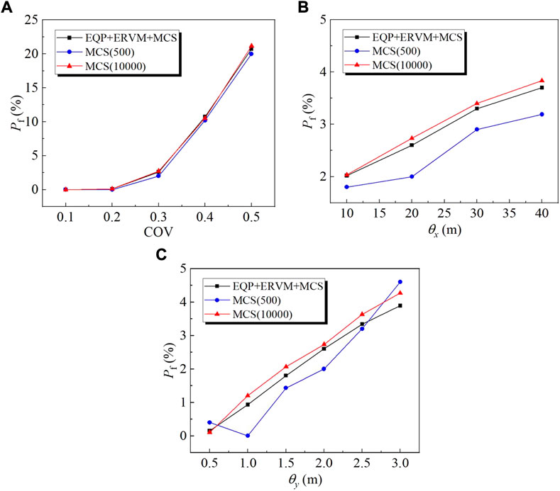
Figure 9 plots the influence of COV, θ_x and θ_y on the reliability results based on the simplified framework. It can be seen from the Figure 9A that P_f increases sharply with COV. This is due to the fact that a higher COV results in a more global heterogeneous random field. In Figures 9B,C, P_f also increases with the correlation length θ_x and θ_y. This is owing to the reason that the larger the correlation length is, the greater the local homogeneity of the random field is. Greater local homogeneity of the random field enlarges the probability of the development of weak surface which are consist of weak zones. When the relieved stress transferred along the weak surface, the larger ground deformation occurs and thus leads to higher P_f. Another reason for the higher P_f is that the larger correlation length will make the variation of the stochastic response larger.

FIGURE 9

FIGURE 9. Parametric study on (A) COV, (B) θ_x, and (C) θ_y.

As COV increases from 0.1 to 0.5, P_f is in a range of 0–25%. In comparison, the variation of the correlation length θ_x and θ_y gives rise to narrower ranges of P_f which are 2–4% and 0–5% respectively. This indicates that P_f affected by COV the most. For the correlation length, as a wider range of P_f is provided in Figure 9C, engineers should be more cautious with determining a reasonable value for θ_y when conducting the reliability analysis.

In Figures 9A–C, the P_f according to MCS (10,000) and the EQP+ERVM+MCS is almost the same. This further verifies the practical applicability of the proposed simplified framework in a wider range of spatial variable characteristics. However, the P_f based on MCS (500) deviates from the former two methods, especially when P_f is lower than 5%. As can be seen in Figure 9A, when the COV=0.4 or 0.5, the P_f predicted by all three methods is almost the same. However, as COV decreases to 0.2 and 0.3, the P_f predicted by EQP+ERVM+MCS shows good consistency with MCS (10,000) whereas the deviation between MCS (500) and MCS (10,000) become significant. For example, when COV=0.2, the P_f predicted by EQP+ERVM+MCS and MCS (10,000) is the same as 0.1%, while P_f predicted by MCS (500) is 0%. It should be noted that it is a unconservative result which ignores the risk of great loss. This is observed in Figures 9B,C more apparently as the P_f in these two figures are basically lower than 5%. The variation trend of P_f with correlation length according to EQP+ERVM+MCS and MCS (10,000) is illustrated the same in these two figures, while the P_f based on MCS (500) varies randomly with the correlation length. This indicates that inadequate MCS times is not applicability when estimating the variation trend of P_f with the spatial variable characteristics.

Example II: A tunnel considering multiple spatially variable parameters

Establish the RVM and RFM

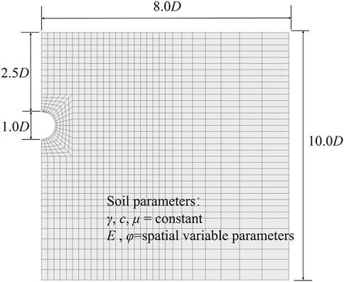
The simplified framework is utilized to estimate the reliability of a tunnel of which the stochastic ground movement is controlled by multiple spatially variable parameters. Figure 10 shows the typical mesh and model domain of the numerical model. The numerical model is modeled by 2,316 element zones and 3,654 grid points. The tunnel diameter is 6 m and the tunnel crown depth is 15 m. Before the stochastic analysis, a sensitivity analysis is carried out to determine the key parameters which influences the S_max the most. A wide range of the influencing parameters are chosen and the value of them are referred to soft soil in the Code for Design of Railway Tunnel (National Rail wayAdministration of the People’s Republic of China, 2016). Forty-four analysis cases are conducted to investigate the key parameters.

FIGURE 10

FIGURE 10. Typical mesh and model domain for example II.

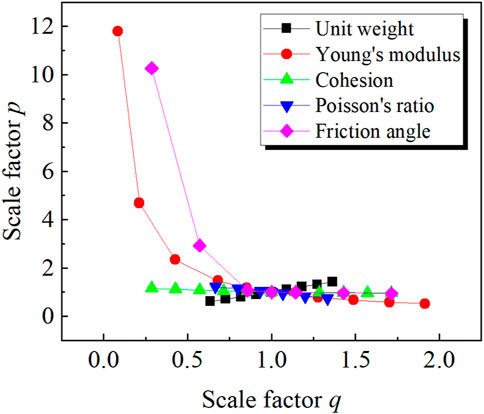
Figure 11 shows the sensitivity analysis results for unit weight γ, young’s modulus E, cohesion c, Poisson’s ratio μ and friction angle φ. In this figure, p denotes the dimensionless scale factor of S_max, which is equal to the S_max divided by the corresponding S_max in the basic case A (γ = 22 kN/m³, E = 23.5 MPa, c = 35 kPa, μ = 0.375, φ = 17.5°). Also, q is dimensionless scale factor of the influencing parameter, which is equal to the influencing parameter divided by the corresponding value in the basic case A. As shown in Figure 11, E and φ have significant effect on S_max, while the effect of γ, c and μ on S_max is insignificant. Therefore, E and φ are the two key parameters that will be analyzed in the following text. Similar to the reliability analysis considering single spatial variability parameter, E and φ are assumed to be subjected to a lognormal stationary anisotropic random field. COV_E is 0.3. The COV of φ (denoted as COV_φ hereafter) is 0.1. For the correlation length, θ_x=20 m and θ_y=2 m are set for both E and φ. The means of E and φ are set as 15° and 20 MPa. The deterministic parameters γ, c and μ are 20 kN/m³, 15 MPa, 0.375 respectively. The stress release ratio is still set as 0.1.

FIGURE 11

FIGURE 11. Sensitivity analysis results.

Determination of the equivalent parameters

Before determining the equivalent parameters, the 247 realizations of RVM are performed to form the dataset for ERVM. The dataset includes the cases with E = {2, 3, 4, 5, 6, 7, 8, 9, 10, 12, 14, 16, 18, 20, 25, 30, 35, 40, 45} MPa and φ = {5, 7, 9, 11, 13, 15, 17, 19, 21, 23, 25, 27, 29} °. Based on the dataset, ERVM is established as:

$\begin{array}{c}{S}_{\mathrm{m}\mathrm{a}\mathrm{x}}\left(E,\phi \right)=k_{\mathit{1}}/E;k_{\mathit{1}}=\mathit{329}\phi -\mathit{4659.6}\phi <\mathit{13}°\\ s_{\max }\left(E,\phi \right)k=k_{\mathit{2}}/E;k_{\mathit{2}}=-\mathit{34808.15}\times e^{-\frac{\phi }{\mathit{2.4}}}-\mathit{227.72},\phi \ge \mathit{13}°\end{array}(7)$

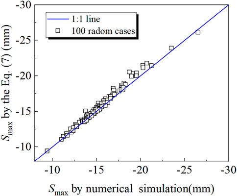
To verify the ERVM, 100 realizations of RVM are conducted. Figure 12 demonstrates the comparison between the S_max values predicted by Eq. 7 and S_max obtained from the RVM. As shown in Figure 12, Eq. 7 is validated to present good performance in predicting the values of S_max.

FIGURE 12

FIGURE 12. Verification of the ERVM by 100 random cases.

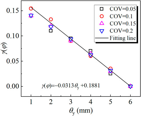
As clarified in the flowchart in Figure 1, when more than one soil parameters are assumed as spatial variable parameters, the strategy including the variance reduction technique introduced in Evaluation of the equivalent parameters should be used. For convenience, φ is the influencing parameter to be reduced. Namely, E is the influencing parameter to be back calculated. To explore the value of variance reduction factor γ(φ), 48 realizations of MCS (10,000) based on RFM are performed. It is found that the effect of COV_φ and θ_x of φ on γ(φ) is small and can be neglected. As a result, the value of γ(φ) can be only related to θ_y and the relationship between γ(φ) and θ_y is shown in Figure 13. As can be seen in Figure 13, γ(φ) decreases as θ_y increases and this can be concluded as:

$\gamma \left(\phi \right)=-0.0313\theta \mathrm{y}+0.18811.(8)$

FIGURE 13

FIGURE 13. The linear relationship between γ(φ) and θ_y.

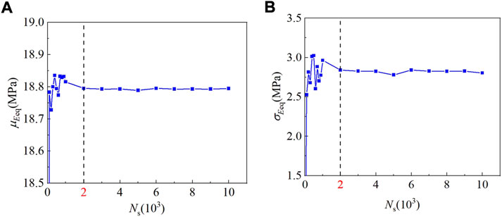
Incorporated with the variance reduction factor γ(φ), the statistics of E_eq and φ_eq can be drawn according to N_s realizations of RFM. Also, as E_eq is the only parameter needs to be back-calculated, the variation of the statistics of E_eq with N_s is analyzed to find a proper N_s. Figure 14 shows the sensitivity study results for the variation of the statistics of E_eq with N_s. As shown in both figures, the statistics varies greatly when N_s is lower than 2000, but this become insignificantly when N_s exceeds 2000. Therefore, N_s =2000 is assumed in this section.

FIGURE 14

FIGURE 14. Variation of (A) μ_Eeq and (B) σ_Eeq with N_s.

Reliability analysis

The definition of MCS, EQP+MCS and EQP+ERVM+MCS are the same as which has been explained in example I. When considering the spatial variability of E and φ, the P_f of MCS, EQP+MCS and EQP+ERVM+MCS are 0.0503, 0.055 and 0.0545 respectively. Good consistency is obtained between three methods and it is verified that the proposed simplified framework also performs well considering multiple spatial variable parameters.

Parametric study

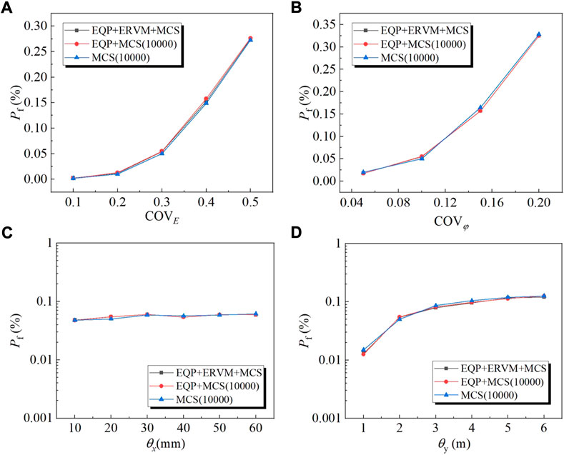
To explore the spatial variability effect of E and φ on the reliability of the ground movement of tunnelling, the correlation length and the coefficient of variation of these 2 parameters are analyzed based on the simplified framework. Also, to verify the simplified framework in a wider range of spatial variable characteristics, the results of MCS (10,000) as well as the EQP+MCS (10,000) are also presented. In the parametric study, θ_x varies from 10 to 60 m with an interval of 10 m whereas θ_y varies from 1.0 to 6.0 m with an interval of 1.0 m. In addition, COV_E ranges from 0.1 to 0.5 with an interval of 0.1 while COV_φ ranges from 0.05 to 0.2 with an interval of 0.05. Only one parameter is changed in the parametric study and the value of the remaining parameters equals to the basic case of which θ_x=20m, θ_y=2.0m, COV_E =0.3 and COV_φ=0.1.

Figure 15 demonstrates the influence of COV_E, COV_φ, θ_x and θ_y on the reliability results based on the simplified framework. It can be seen from the Figures 15A,B that P_f increases sharply with COV_E and COV_φ. However, P_f is more sensitive to the COV_φ than COV_E. This is reasonable since the φ controls the plastic deformation of soil. Moreover, the P_f evaluated by the proposed simplified framework agrees well with the EQP+MCS (10,000) and MCS (10,000). In particular, the proposed simplified framework predicts accurate P_f at low probability levels such as COV_E =0.1 or COV_φ = 0.05. When COV_E =0.1, P_f estimated by the proposed simplified framework is 0.00265, which is comparable to the P_f based on MCS (10,000) with a value of 0.002. Also, when COV_φ = 0.05, P_f estimated by the proposed simplified framework is 0.01754, which is comparable to the P_f based on MCS (10,000) with a value of 0.02. As shown in Figures 15C,D, P_f increases with θ_y nonlinearly, whereas seldomly changes when θ_x varies. Overall, the proposed simplified framework shows practical applicability in predicting the reliability considering multiple parameters in a wide range of spatial variable characteristics.

FIGURE 15

FIGURE 15. Parametric study on (A) COV_E, (B) COV_φ, (C) θ_x, and (D) θ_y.

Conclusion

This study presents a more reasonable and efficient reliability analysis for ground movement of tunnelling in spatial variable soil by incorporating with the equivalent parameters. The proposed simplified framework utilized in this study refers to Liu et al. (2018) which is firstly introduced in slope stability analysis. The theoretical basis and the detailed process are explained thoroughly in this study. Reliability analysis is conducted on both tunnels considering single and multiple spatial variable parameters. By comparing to the former study (Cheng et al., 2019b) and direct MCS on RFM, the proposed simplified framework is verified to show good performance in evaluating the P_f of ground movement of tunnelling. Parametric study is carried out to figure out the effect of various parameters related to spatial variability on the P_f. The conclusions in this study are drawn as:

1) The proposed simplified framework can effectively address the reliability analysis for ground movement of tunnelling in spatially variable soils. Compared to the previous study, the P_f of ground movement of tunnelling is more accurate and reliable. Its accuracy is maintained for an anisotropic random field with wider range of the correlation lengths and COV of various parameters. This indicates that the proposed simplified framework is a applicable tool in estimating the P_f of ground movement of tunnelling.

2) The young’s modulus E of the soil is assumed as a spatial variable parameter in tunnel first. When considering the spatial variability of E, P_f increases sharply with the COV of E. P_f also increases with the correlation length. However, P_f is sensitive to the COV of E most. Compared to θ_x, θ_y influences the P_f more significantly.

3) According to the results of the 44 sensitivity analysis cases, the young’s modulus E and the friction angle φ are assumed as the spatial variable parameters in a tunnel considering multiple spatial variable parameters. In comparison, the unit weight γ, the cohesion c and the Poisson ratio μ show limited impact on the ground movement and their spatial variability is neglected in the tunnel case considering multiple spatial variable parameters.

4) Before conducting the reliability analysis considering the spatial variability of E and φ, the reduction factor γ(φ) is discussed based on 48 realizations of MCS (10,000). As a result, the value of γ(φ) can be only related linearly to the vertical correlation length θ_y but is uncorrelated with the horizontal correlation length θ_x. The linear relationship between γ(φ) and θ_y can be expressed as Eq. 8.

5) Parametric study of the reliability analysis considering the spatial variability of E and φ indicates that the COV_φ produce greater effect on P_f than the COV_E. Differing from the reliability analysis considering the effect of single spatial variable, P_f increases nonlinear with θ_y but stays almost constant with θ_x.

Data availability statement

The original contributions presented in the study are included in the article/supplementary material, further inquiries can be directed to the corresponding author.

Author contributions

WY: Methodology, Formal analysis, Writing—original draft. HL: Conceptualization, Writing—review and editing. JZ: Supervision, Resources. LC: Investigation, Software.

Funding

The authors acknowledge the financial support provided by the National Natural Science Foundation of China (No. 51878313, No. 52078236).

Conflict of interest

The authors declare that the research was conducted in the absence of any commercial or financial relationships that could be construed as a potential conflict of interest.

Publisher’s note

All claims expressed in this article are solely those of the authors and do not necessarily represent those of their affiliated organizations, or those of the publisher, the editors and the reviewers. Any product that may be evaluated in this article, or claim that may be made by its manufacturer, is not guaranteed or endorsed by the publisher.

References

Cami, B., Javankhoshdel, S., Phoon, K. K., and Ching, J. (2021). Erratum for “scale of fluctuation for spatially varying soils: Estimation methods and values” by brigid cami, sina Javankhoshdel, kok-kwang Phoon, and jianye ching. ASCE-ASME J. Risk Uncertain. Eng. Syst. Part A Civ. Eng. 7 (4), 08221001. doi:10.1061/ajrua6.0001194

CrossRef Full Text | Google Scholar

Cami, B., Javankhoshdel, S., Phoon, K. K., and Ching, J. (2020). Scale of fluctuation for spatially varying soils: Estimation methods and values. ASCE-ASME J. Risk Uncertain. Eng. Syst. Part A Civ. Eng. 6 (4). doi:10.1061/ajrua6.000108303120002

CrossRef Full Text | Google Scholar

Chakeri, H., Ozcelik, Y., and Unver, B. (2013). Effects of important factors on surface settlement prediction for metro tunnel excavated by EPB. Tunn. Undergr. Space Technol. 36, 14–23. doi:10.1016/j.tust.2013.02.002

CrossRef Full Text | Google Scholar

Cheng, H., Chen, J., Chen, R., Huang, J., and Li, J. (2019a). Three-dimensional analysis of tunnel face stability in spatially variable soils. Comput. Geotech. 111, 76–88. doi:10.1016/j.compgeo.2019.03.005

CrossRef Full Text | Google Scholar

Cheng, H., Chen, J., and Li, J. (2019b). Probabilistic analysis of ground movements caused by tunneling in a spatially variable soil. Int. J. Geomech. 19 (12), 04019125–4019210. doi:10.0401912510.1061/(ASCE)GM.1943-5622.0001526

CrossRef Full Text | Google Scholar

Ching, J. Y., Phoon, K. K., and Kao, P. H. (2014). Mean and variance of mobilized shear strength for spatially variable soils under uniform stress states. J. Eng. Mech. 140 (3), 487–501. doi:10.1061/(asce)em.1943-7889.0000667

CrossRef Full Text | Google Scholar

Cui, L., Sheng, Q., Dong, Y. K., and Xie, M. X. (2021a). Unified elasto-plastic analysis of rock mass supported with fully grouted bolts for deep tunnels. Int. J. Numer. Anal. Methods Geomech. 46, 247–271. doi:10.1002/nag.3298

CrossRef Full Text | Google Scholar

Cui, L., Sheng, Q., Dong, Y., Ruan, B., and Xu, D. D. (2021b). A quantitative analysis of the effect of end plate of fully-grouted bolts on the global stability of tunnel. Tunn. Undergr. Space Technol. 114 (2), 104010. doi:10.1016/j.tust.2021.104010

CrossRef Full Text | Google Scholar

Dasaka, S. M., and Zhang, L. M. (2012). Spatial variability of in situ weathered soil. Geotechnique 62 (5), 375–384. doi:10.1680/geot.8.P.151.3786

CrossRef Full Text | Google Scholar

Dong, Y. K., Cui, L., and Zhang, X. (2022). Multiple-GPU parallelization of three-dimensional material point method based on single-root complex. Int. J. Numer. Methods Eng. 123 (6), 1481–1504. doi:10.1002/nme.6906

CrossRef Full Text | Google Scholar

Eshraghi, A., and Zare, S. (2015). Face stability evaluation of a TBM-driven tunnel in heterogeneous soil using a probabilistic approach. Int. J. Geomech. 15 (6), 4014095–4014101. doi:10.1061/(ASCE)GM.1943-5622.0000452

CrossRef Full Text | Google Scholar

Griffiths, D. V., Fenton, G. A., and Manoharan, N. (2006). Undrained bearing capacity of two-strip footings on spatially random soil. Int. J. Geomech. 6 (6), 421–427. doi:10.1061/(ASCE)1532-3641(2006)6:6(421)

CrossRef Full Text | Google Scholar

Griffiths, D. V., and Fenton, G. A. (2004). Probabilistic slope stability analysis by finite elements. J. Geotech. Geoenviron. Eng. 130 (5), 507–518. doi:10.1061/(asce)1090-0241(2004)130:5(507)

CrossRef Full Text | Google Scholar

Griffiths, D. V., Huang, J., and Fenton, G. A. (2009). Influence of spatial variability on slope reliability using 2-d random fields. J. Geotech. Geoenviron. Eng. 135 (10), 1367–1378. doi:10.1061/(ASCE)GT.1943-5606.0000099

CrossRef Full Text | Google Scholar

Huang, L., and Leung, Y. F. (2021). Reliability assessment of slopes with three dimensional rotated transverse anisotropy in soil properties. Can. Geotech. J. 58 (9), 1365–1378. doi:10.1139/CGJ-2019-0611

CrossRef Full Text | Google Scholar

Javankhoshdel, S., Luo, N., and Bathurst, R. J. (2017). Probabilistic analysis of simple slopes with cohesive soil strength using RLEM and RFEM. Georisk Assess. Manag. Risk Eng. Syst. Geohazards 11 (3), 231–246. doi:10.1080/17499518.2016.1235712

CrossRef Full Text | Google Scholar

Jiang, S. H., Li, D. Q., Cao, Z. J., Zhou, C. B., and Phoon, K. K. (2015). Efficient system reliability analysis of slope stability in spatially variable soils using monte carlo simulation. J. Geotech. Geoenviron. Eng. 141 (2), 04014096. doi:10.1061/(ASCE)GT.1943-5606.0001227

CrossRef Full Text | Google Scholar

Jiang, S. H., Li, D. Q., Zhang, L. M., and Zhou, C. B. (2014). Slope reliability analysis considering spatially variable shear strength parameters using a non-intrusive stochastic finite element method. Eng. Geol. 168, 120–128. doi:10.1016/j.enggeo.2013.11.006

CrossRef Full Text | Google Scholar

Kiureghian, A. D., and Ke, J. B. (1988). The stochastic finite element method in structural reliability. Probabilistic Eng. Mech. 3 (2), 83–91. doi:10.1016/0266-8920(88)90019-7

CrossRef Full Text | Google Scholar

Lee, K. M., and Rowe, R. K. (1990). Finite element modelling of the three-dimensional ground deformations due to tunnelling in soft cohesive soils: Part I—method of analysis. Comput. Geotech. 10 (2), 87–109. doi:10.1016/0266-352x(90)90001-c

CrossRef Full Text | Google Scholar

Li, D. Q., Jiang, S. H., Cao, Z. J., Zhou, W., Zhou, C. B., and Zhang, L. M. (2015). A multiple response-surface method for slope reliability analysis considering spatial variability of soil properties. Eng. Geol. 187, 60–72. doi:10.1016/j.enggeo.2014.12.003

CrossRef Full Text | Google Scholar

Li, D. Q., Xiao, T., Cao, Z. J., Zhou, C. B., and Zhang, L. M. (2016). Enhancement of random finite element method in reliability analysis and risk assessment of soil slopes using Subset Simulation. Landslides 13, 293–303. doi:10.1007/s10346-015-0569-2

CrossRef Full Text | Google Scholar

Liu, L. L., Deng, Z. P., Zhang, S. H., and Cheng, Y. M. (2018). Simplified framework for system reliability analysis of slopes in spatially variable soils. Eng. Geol. 239, 330–343. doi:10.1016/j.enggeo.2018.04.009

CrossRef Full Text | Google Scholar

Liu, W. K., Belytschko, T., and Mani, A. (1986). Random field finite elements. Int. J. Numer. Methods Eng. 23 (10), 1831–1845. doi:10.1002/nme.1620231004

CrossRef Full Text | Google Scholar

Loganathan, N., and Poulos, H. G. (1998). Analytical prediction for tunneling-induced ground movements in clays. J. Geotech. Geoenviron. Eng. 124 (9), 846–856. doi:10.1061/(asce)1090-0241(1998)124:9(846)

CrossRef Full Text | Google Scholar

Luo, Z., Atamturktur, S., and Cai, Y. (2012). Reliability analysis of basal-heave in a braced excavation in a 2-D random field. Comput. Geotech. 39, 27–37. doi:10.1016/j.compgeo.2011.08.005

CrossRef Full Text | Google Scholar

Migliazza, M., Chiorboli, M., and Giani, G. P. (2009). Comparison of analytical method, 3D finite element model with experimental subsidence measurements resulting from the extension of the Milan underground. Comput. Geotech. 36 (1-2), 113–124. doi:10.1016/j.compgeo.2008.03.005

CrossRef Full Text | Google Scholar

Miro, S., Koenig, M., and Hartmann, D. A. (2015). Probabilistic analysis of subsoil parameters uncertainty impacts on tunnel-induced ground movements with a back-analysis study. Comput. Geotech. 68, 38–53. doi:10.1016/j.compgeo.2015.03.012

CrossRef Full Text | Google Scholar

Mollon, G., Dias, D., and Soubra, A. H. (2012). Probabilistic analyses of tunneling-induced ground movements. Acta Geotech. 8 (2), 181–199. doi:10.1007/s11440-012-0182-7

CrossRef Full Text | Google Scholar

Mollon, G., Dias, D., and Soubra, A. H. (2013). Range of the safe retaining pressures of a pressurized tunnel face by a probabilistic approach. J. Geotech. Geoenviron. Eng. 139, 1954–1967. doi:10.1061/(ASCE)GT.1943-5606.0000911

CrossRef Full Text | Google Scholar

National Railway Administration of the People' Republic of China. (2016). TB10003-2016, Code for Design of Railway tunnel. China Railway Press, Beijing: China.

Google Scholar

Pan, Q., and Dias, D. (2017). Probabilistic evaluation of tunnel face stability in spatially random soils using sparse polynomial chaos expansion with global sensitivity analysis. Acta Geotech. 12 (6), 1415–1429. doi:10.1007/s11440-017-0541-5

CrossRef Full Text | Google Scholar

Peck, R. B. (1969). Deep excavations and tunneling in soft ground. Mexico: Proc. of 7th ICSMFE.

Google Scholar

Phoon, K. K., Huang, S. P., and Quek, S. T. (2002). Implementation of Karhunen–Loeve expansion for simulation using a wavelet-Galerkin scheme. Probabilistic Eng. Mech. 17 (3), 293–303. doi:10.1016/S0266-8920(02)00013-9

CrossRef Full Text | Google Scholar

Phoon, K. K., and Kulhawy, F. H. (1999). Characterization of geotechnical variability. Can. Geotech. J. 36 (4), 612–624. doi:10.1139/t99-038

CrossRef Full Text | Google Scholar

Stuedlein, A. W., Cami, B., Curzio, D. D., Javankhoshdel, S., Nishumura, S., Pula, W., et al. (2021). Summary of random field model parameters of geotechnical properties. TC304 State-of-the-art Rev. Inherent Var. Uncertain. Geotechnical Prop. Models, 95

Google Scholar

Tabarroki, M., Ching, J., Lin, C. P., Liou, J. J., and Phoon, K. K. (2022b). Homogenizing spatially variable Young modulus using pseudo incremental energy method. Struct. Saf. 97, 102226. doi:10.1016/j.strusafe.2022.102226

CrossRef Full Text | Google Scholar

Tabarroki, M., Ching, J., Phoon, K. K., and Chen, Y. Z. (2022a). Mobilisation based characteristic value of shear strength for ultimate limit states. Georisk Assess. Manag. Risk Eng. Syst. Geohazards, 1–22. doi:10.1080/17499518.2020.1859121

CrossRef Full Text | Google Scholar

Vanmarcke, E. H. (2010). Random fields: Analysis and synthesis. Revised and expanded. New Edition. Beijing, China: World Scientific Publishing.

Google Scholar

Wang, Y., Cao, Z., and Au, S. K. (2010). Practical reliability analysis of slope stability by advanced monte carlo simulations in a spreadsheet. Can. Geotech. J. 48, 162–172. doi:10.1139/T10-044

CrossRef Full Text | Google Scholar

Zhang, R. J., Zheng, J. J., and Dong, Y. K. (2011). Elaborate simulation method for the influence of soil excavation of shield tunnels on existing pile foundations. Adv. Mat. Res. 168, 270–275. doi:10.4028/www.scientific.net/AMR.168-170.270

CrossRef Full Text | Google Scholar