Using sequential conditioning to explore uncertainties in geostatistical characterization and in groundwater transport predictions

Rapid transmission of contaminants in groundwater can occur in alluvial gravel aquifers that are permeated by highly conductive small-scale open framework gravels (OFGs). This open framework gravel structure and the associated distribution of hydraulic properties is complex, and so assessments of contamination risks in these aquifers are highly uncertain. Geostatistical models, based on lithological data, can be used to quantitatively characterize this structure. These models can then be used to support analyses of the risks of contamination in groundwater systems. However, these geostatistical models are themselves accompanied by significant uncertainty. This is seldom considered when assessing risks to groundwater systems. Geostatistical model uncertainty can be reduced by assimilating information from hydraulic system response data, but this process can be computationally challenging. We developed a sequential conditioning method designed to address these challenges. This method is demonstrated on a transition probability based geostatistical simulation model (TP), which has been shown to be superior for representing the connectivity of high permeability pathways, such as OFGs. The results demonstrate that the common modelling practice of adopting a single geostatistical model may result in realistic predictions being overlooked, and significantly underestimate the uncertainties of groundwater transport predictions. This has important repercussions for uncertainty quantification in general. It also has repercussions if using ensemble-based methods for history matching, since it also relies on geostatistical models to generate prior parameter distributions. This work highlights the need to explore the uncertainty of geostatistical models in the context of the predictions being made.

1 Introduction

Alluvial gravel aquifers are a valuable source of freshwater globally (Alsharhan and Rizk, 2020; De Luca et al., 2020). Due to their alluvial nature, such aquifers are inherently heterogeneous, being composed of various sedimentary textural classes that include open framework gravels (OFGs) (Cary, 1951; Lunt et al., 2004; Bridge & Lunt, 2006; Lunt & Bridge, 2007). A characteristic trait of OFGs is their macroporosity, which makes them highly permeable (Klingbeil et al., 1999; Ferreira et al., 2010). Dann et al. (2008), and Jussel et al. (1994) have shown through field tests and numerical modelling that the connectedness of OFGs has a profound effect on the hydraulic function of alluvial gravel aquifers, by facilitating preferential flow and rapid solute transport. OFGs also have a low capacity for microbial removal (Rossi et al., 1994; Pang, 2009; Flynn et al., 2015) and therefore pose a significant risk in regard to human exposure to pathogenic disease in situations where untreated drinking water is sourced from alluvial gravel aquifers. The 2016 [ground]waterborne Campylobacteriosis outbreak (around 7,000 cases) that occurred at Havelock North, New Zealand is a case example (Government Inquiry into Havelock North Drinking Water, 2017; Gilpin et al., 2020).

The work presented in this paper was motivated by the need for robust methods to evaluate groundwater contamination risks associated with alluvial gravel aquifer settings that incorporate OFG. Robust model-based assessments of contaminant risk in these groundwater systems are based on geostatistical models that characterize the structure of these rapid transport pathways. In this paper we focus on the geostatistical characterization of these most permeable pathways, and the implications of uncertainty in this characterization.

1.1 Geostatistical methods in hydrogeological modelling

There are many practical limitations to mapping the structure of alluvial gravels at a resolution that can detect OFGs. Heterogeneous aquifer datasets are almost always sparse and incomplete, particularly in lateral dimensions (Sanchez-Vila & Fernandez-Garcia, 2016). Consequently, stochastic inversion methods, even when coupled with distributed parameterizations, are unlikely to identify small-scale highly heterogeneous pathways (Doherty & Moore, 2021). Because of this, we use stochastic frameworks to characterize heterogeneity structure, based on geostatistical or physical process-based modelling methods (e.g. Riva et al., 2006; Riva et al., 2008; Ritzi & Soltanian, 2015; Scheibe et al., 2015; Siena & Riva, 2020).

Physical process-based modelling methods simulate structural aspects of alluvial deposits based on probabilistic representations of lithological categories within a meandering river geometry, and are informed by the sedimentary disposition of the system. Examples include BCS-3D (Webb & Anderson, 1996), FLUVSIM (Deutsch & Tran, 2002) and ALLUVSIM (Pyrcz et al., 2009). Geostatistical models can be based on covariance or variogram structures for continuously variable hydraulic properties (Deutsch & Journel, 1998). Other options, such as training image methods, including Multiple-Point Statistics, can be used to represent more complex geological environments that cannot be fully represented by two-point covariance relationships (Strebelle, 2002; Huysmans & Dassargues, 2009).

Where sharp interfaces occur between high and low conductivity media, such as in aquifers with OFGs, geostatistical models based on categorical variables can be used to generate realizations of aquifer media. Categorical methods include Sequential Indicator Simulation (SIS) which relies on indicator variograms based on borehole lithological data (Goovaerts, 1997; Deutsch & Journel, 1998), and Transition Probability (TP) Simulation (Carle, 1999). TP simulation has the advantage that it honors volumetric proportions, mean dimensions and the connectivity patterns of the categorical variables.

The choice of the most appropriate structural model of heterogeneity largely depends on the features that control the predictive response of concern (e.g., Jafarpour & Tarrahi, 2011; Ciriello et al., 2013; Riva et al., 2015). We opted to use TP simulation which has been shown to be superior for representing the connectivity of high permeability pathways (Siena & Riva, 2020). TP simulation is also well-established and used in numerous modelling studies, including groundwater modelling studies, that rely on a geostatistical description of the spatial dependencies of selected categories (e.g. Park et al., 2004; Engdahl & Weissmann, 2010; Hansen et al., 2014; He et al., 2014).

1.2 Direct and indirect data and sequential conditioning

The sparsity of information with which to develop geostatistical models of heterogeneity structure has motivated efforts to combine ‘direct’ observations made of mapped lithological properties with ‘indirect’ data (Refsgaard et al., 2012; Carle & Fogg, 2020) that require another level of interpretation that carries with it uncertainty. Pumping test data (Harp et al., 2008; Harp and Vessilinov, 2010; Harp & Vessilinov, 2012) and geophysical data (Engdahl & Weissmann, 2010; Koch, 2013; He et al., 2014; Zhu et al., 2016) are examples of ‘indirect’ observational data often used to condition and reduce the uncertainty of geostatistical models. Indirect data relating to dynamical physical processes such as flow and transport can be extremely informative, since they provide a measure of connectivity within the hydrogeological model (Renard and Allard, 2013).

Using information from indirect hydrogeologic data can nonetheless impose a significant computational burden, as this involves the comparison of field observations with groundwater model simulation outputs within a stochastic or Bayesian workflow (Jafarpour & Tarrahi, 2011; Ciriello et al., 2013; Linde et al., 2015; Riva et al., 2015). Selection of the conditioning method can also be problematic, potentially degrading the geological realism of the conditioned realizations when spatially distributed parameters are adjusted in order to provide a match to field observations (Oliveira et al., 2017; Chan & Elsheikh, 2020).

Sequential conditioning can be used to address the computational burden described above, where some data requires more computational processing effort than others (Feyen et al., 2003; Hassan et al., 2009; Dorn et al., 2012). Sequential conditioning commences by history matching to datasets that require the least computational effort. Each subsequent conditioning step is focused on a selection of observations requiring increasingly greater computational processing. Using this process allows the prior distribution to gradually morph into a posterior distribution. We develop an approach that harnesses the strengths, and mitigates the weaknesses, of two distinct conditioning methods: stochastic inversion and rejection sampling.

The stochastic inversion method uses a history matching approach to condition the TP model parameters through minimizing the residuals between the transition probabilities derived from the TP geostatistical model and those derived from the direct lithological data. The TP model parameters are further conditioned using “greater than” and “less than” constraints, via a rejection sampling methodology applied to the indirect observations.

Conditioning of geostatistical models is easier to discuss when adopting Bayesian nomenclature (Kennedy and O'Hagan, 2002). Therefore, in the sections that follow the geostatistical model parameters (facies lengths, and volumetric proportions) are referred to as ‘hyperparameters’, to distinguish them from ‘model parameters’ i.e., hydraulic properties of the underlying aquifer system being analyzed. Probability density functions of hyperparameters are thus used to describe the uncertainty of the geostatistical model. Note that if alternative geostatistical models were adopted the hyperparameters would differ: e.g. for a variogram based geostatistical model, the hyperparameters would comprise the sill, range and nugget parameters.

1.3 Research objectives

This paper explores the implications of geostatistical model uncertainty for a particle transport modelling problem in an alluvial gravel aquifer, where transport function is determined by the connected, small-scale OFG textural class (Dann et al., 2008; Burbery et al., 2017; Theel et al., 2020). It also demonstrates the potential of a Sequential Conditioning Approach, using a case study which contains a uniquely detailed field dataset (consisting of direct and indirect observations) that was initially described by Burbery et al. (2017). This case study includes data from novel smoke tracing experiments designed to characterize the connectivity of OFG pathways. These data are particularly valuable, given the advantages of conditioning to prediction-salient information (White et al., 2014; Doherty, 2015). Using the geostatistical model hyperparameter distribution derived from the analysis, we explored the predictive implications of the common practice of adopting a single most likely geostatistical model to underpin a groundwater contamination risk assessment.

The structure of the paper is as follows: in Section 2 we provide some background to the case study field site and describe the direct and indirect field observational datasets that were compiled for the alluvial gravel aquifer model used in the study. The mathematical methodologies and framework developed and tested in this study are described in Section 3. In Section 4 we present the results from our modelling analyses, whilst also exploring and discussing some implications that the equifinality of structural heterogeneity models have for predictions of travel time in alluvial gravel aquifers. Section 5 presents our conclusions and discusses implications of these for stochastic decision support modelling in practice.

2 Case study

The Canterbury Plains aquifer on the South Island, New Zealand (NZ) covers an area of approximately 8,000 km² and consists of sets of coalesced alluvial fans that were active during the Quaternary period (Leckie, 1994; Bal, 1996; Ashworth et al., 1999; Browne & Naish, 2003; Leckie, 2003). This extensive aquifer, used for irrigation, industrial and potable water supply (Bal, 1996; Brown, 2001) is ranked as the most valuable groundwater resource in NZ (White, 2001). The general sedimentary structure of the aquifer is characteristic of gravel outwash deposits formed from large braided-river systems. The Kyle field site (43.94338 S, 172.06788 E), from which the observational datasets used in this study were obtained, is located on the Rakaia River fan, on the coastal boundary of the Canterbury Plains. At the last glacial maxima, the site would have been positioned approximately mid-point on the Rakaia fan (Browne & Naish, 2003).

2.1 Lithological mapping (direct observational data)

A 3D portion of the alluvial deposits at Kyle has been mapped, covering an area measuring 28 m x 20 m and to a depth of 6 m below the Rakaia fan surface. Mapping was conducted from two cliff exposures (a sea cliff oriented perpendicular to the presumed paleoflow direction and a ‘donga’, i.e. a steep-sided gully created by soil erosion, with a face aligned 90° to the sea cliff), and nine large (1.2 m) diameter boreholes (coded K1 to K9) that were drilled 5 m apart on a 3x3 uniform grid, 18 m inland from the cliffs (see Figure 1 inset). The lithological examination is limited to the unsaturated zone. However, these vertically-stacked gravel packages mapped near the surface at Kyle represent a sample of the alluvial sequence that forms the Canterbury Plains aquifer system. Therefore we are able to make the assumption that this sample provides a useful analogue model of a saturated gravel aquifer system. Further details of the Kyle field site and investigative methods are provided in Burbery et al. (2017).

FIGURE 1

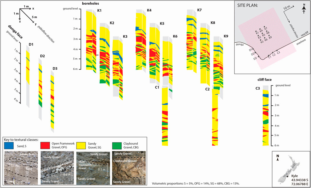
FIGURE 1. Box plot map of the Kyle site showing the spatial distribution of the four main lithological categories (textural classes), as identified on cliff exposures and borehole walls. Site location, and the model domain and grid that is used in the geostatistical and groundwater modelling analyses, are shown in inset of site plan. Representative photographic images of textural classes are included in the legend.

Employing descriptive methods such as those described by Koltermann & Gorelick (1996), Burbery et al. (2017) compiled a map of the Kyle site adopting four lithological categories, being: sand (S); sandy gravel (SG); open framework gravel (OFG) and clay-bound gravel (CBG). Photographic examples of the four lithological categories, as imaged at Kyle, are presented in Figure 1. Particle size distribution data, and a description of the geological depositional history for this alluvial system can be found in Burbery et al. (2017). The relative compositions of the lithological categories at the Kyle site are: S 5.1%, SG 67.8%, OFG 14.2% and CBG 12.9%.

OFG at the Kyle site predominantly occur as cross-strata comprising packaged sets of alternating OFG and SG. The thickness of the OFG lithological category is dependent on the angle of the foresets and was observed to vary between 0.2 m and 1 m. The lateral extent of OFG seen in cliff exposures was more than 25 m in some cases. Although less common, OFGs at Kyle also feature as planar beds up to 0.3 m thick and 4 m–5 m wide. From exposures observed on the donga face that is orientated along the paleoflow direction, it is apparent that the planar beds can extend for at least 15 m in length (Burbery et al., 2017).

On the basis of pumping and tracer test data, Dann et al. (2008) established that typical hydraulic conductivities of OFG in the Canterbury Plains alluvial aquifer system are two to three orders of magnitude greater (i.e. more permeable) than those of the other three categories (i.e. OFG have a saturated conductivity of 1,498–10,646 m/day compared with a range for the other three categories from 5.5 to 117.28 m/day). This is consistent with Klingbeil et al. (1999) who described the average hydraulic conductivity of OFG being around 100 times greater than the other alluvial categories studied. Dann et al. (2008) estimated that this hydraulic conductivity contrast between lithological categories results in approximately 98% of aquifer flow occurring through these permeable connected OFGs. Therefore, it is the connectivity of these rapid transport OFG pathways that is relevant to the representation of pathogen transport in aquifers (Fiori et al., 2013; Hunt & Johnson 2017).

We adopt a ‘forecast first’ approach to the development of the geostatistical model (Doherty 2015; White 2017) and focus our analysis on the connectivity of the OFG category identified from observations to generate random realizations of the OFG and other lithological categories at the scale of the numerical grid. Assignment of hydraulic conductivity values reflected the order of magnitude differences in conductivity between the most permeable (OFG) and the next most permeable facies (S, SG, CBG), resulting in a binary characterization of the hydraulic properties within the aquifer system. While at first glance this grouping may seem to overly simplify the geological characterization described in Burbery et al. (2017), this simplification has no impact on the predictions we are making, given the contrast in permeability between the OFG and the other lithological categories, which are considered to be analogous to hydrofacies (Soltanian & Ritzi, 2014; Theel et al., 2020).

2.2 Smoke tracer tests to determine connectivity of OFG (indirect observational data)

Three smoke tracer tests were conducted using the array of open boreholes described to examine the interconnectedness of OFGs at Kyle. The tests are documented in detail in Burbery et al. (2017). In brief, they involved injecting smoke under a low positive pressure into each of the centrally-located boreholes K2, K5 and K8 for an extended period. The arrival time and position of smoke emerging from OFG in neighboring boreholes was then recorded. The results of the smoke experiments confirmed that OFGs are truly ‘open’ since smoke was able to travel rapidly between boreholes through OFGs. Connectivity was found to be non-uniform in direction, reflecting both the heterogeneity and anisotropy of the alluvial sediments. Figure 2 illustrates the connectivity between OFGs, as inferred from the three smoke tracer tests at boreholes K2, K5 and K8.

FIGURE 2

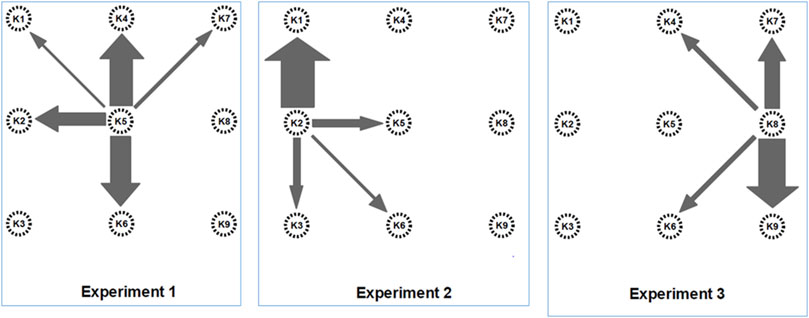
FIGURE 2. Schematic of smoke tracer test results. Arrows indicate connections between injection boreholes and observation points. The width of the arrows indicates the relative strength of those connections of high conductivity pathways as inferred from the observed arrival times.

The earliest arrival time for smoke transmitted between two boreholes located 5 m apart was 48 s, along a co-set of planar OFG strata running between K2 and K1 that were aligned with the paleoflow direction. For all tests, fastest velocities corresponded to the mean paleoflow direction, i.e. NNW-SSE or y-direction (Figure 1). In some cases, no smoke was detected to have travelled between adjacent boreholes, suggestive of no apparent connectivity between the observed OFG strata. When transmission between boreholes occurred, the latest observed smoke arrival time was 30 min, between boreholes K5 and K1. A specific result of the smoke tracer tests was the lack of any observable hydraulic connection between OFG in test borehole K5 and OFG mapped in both K8 and K9, to the north (Figure 2).

The lithological data from borehole-logs, outcrops and geological characterization (Figure 1), and the observed cross-borehole connectivity from these smoke tracer experiment results (Figure 2), provided the respective direct, and indirect, observational data that were used to derive the geostatistical model of the most permeable and least permeable categories in this aquifer structure. The following sections describe the processes and mathematical methods that utilized these different types of information.

3 Methodology

3.1 Sequential conditioning of heterogeneity structure models

The sequential conditioning approach provides a Monte Carlo implementation of Bayes theorem and involves a sequence of history matching steps. The initial step focusses on the data which is the most rapid to process. Subsequent conditioning steps are only applied to those parameter ranges identified as plausible from the preceding step, and targets data that is increasingly slower to process. The approach has computational advantages over joint inversion if assimilating information from multiple datasets with one dataset involving a simulation model with long run times (Feyen et al., 2003; Hassan et al., 2009).

Previous sequential conditioning studies have adopted a single conditioning approach (Feyen et al., 2003; Hassan et al., 2009; Dorn et al., 2012). We combine two stochastic inversion approaches to further reduce the computation burden of history matching to disparate datasets. Computationally efficient stochastic inversion methods, such as randomized maximum likelihood approaches, are used to condition observation groups where possible. However, rejection sampling is used if stochastic inversion risks degrading the representation of important spatially defined geological features, such as a connected flow pathway, as demonstrated by Dorn et al. (2012) with observations of cross-borehole connectivity in a fractured rock aquifer. While rejection sampling is too computationally inefficient for most groundwater modelling contexts, this burden is alleviated when using it only in final conditioning steps (Dorn et al., 2012; Linde et al., 2015; Cirpka & Valocchi, 2016; Carle & Fogg, 2020). In this way the different strengths of conditioning methods can be employed where appropriate, while the respective weaknesses of each method are mitigated.

We applied this sequential conditioning approach using direct and indirect geological observations. Direct observations were comprised of lithological log data and were processed using a stochastic inversion approach. Indirect observations of cross-borehole connectivity, derived from the case study tracer test, were processed using rejection sampling.

3.2 Geostatistical model

Geostatistical models based on transition probability (TP) simulation are used in a number of fields (e.g. Huang et al., 2017; Li & Zhang, 2019) to characterize the distribution and juxtapositional characteristics of heterogeneity, such as the connected high permeability features of interest to this case study. We adopted the T-PROGS software for our TP model implementation (Carle (1999), which has been used widely in the hydrogeological field. Carle (1999) defines a transition probability, t_ij, as:

‘Given that a facies j is present at location x, what is the probability that another (or the same) facies i occurs at location x+h’, or:

${\mathit{t}}_{\mathit{i}\mathit{j}}\left(\mathit{h}\right)=\mathit{P}\left\{\mathit{j}\mathit{o}\mathit{c}\mathit{c}\mathit{u}\mathit{r}\mathit{s}\mathit{a}\mathit{t}\mathit{x}+\mathit{h}|\mathit{i}\mathit{o}\mathit{c}\mathit{c}\mathit{u}\mathit{r}\mathit{s}\mathit{a}\mathit{t}\mathit{x}\right\}(1)$

Borehole-log and outcrop data is catalogued into categories, at regular depth intervals, allowing the juxtapositional probabilities of lithological categories to be calculated. These are summarized in matrices of transition probabilities at specific lags (h), in the vertical (z) and horizontal directions, i.e. along the mean paleoflow direction (y or dip direction) and transverse to this direction (x or strike direction). The collation of these transition probabilities at specified separation distances (lags) can also be depicted as a transiogram (Figure 5). These transition probability matrices form the lithological constraints in the sequential conditioning approach.

FIGURE 5

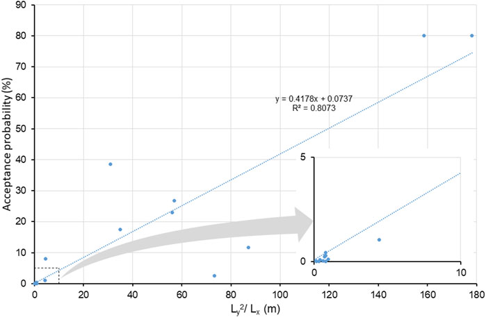
FIGURE 5. Relationship between the proportion of realizations meeting the smoke tracer plausibility test (Acceptance probability) and a ratio L_y²/L_x, which is the squared OFG category mean length in the paleoflow direction (L_y) and perpendicular to the paleoflow direction (L_x). This relationship is shown for 21 TP models examined for the Kyle case study as summarized in Table 1.

From Carle & Fogg (1997), the mean length $\overline{L}$ of the ith category unit in a particular direction can be calculated as:

${\overline{\mathit{L}}}_{\mathit{i}}=\frac{\mathbf{1}}{{\mathit{r}}_{\mathit{i}\mathit{i}}}={\left[\frac{\partial {\mathit{t}}_{\mathit{i}\mathit{i}\left(\mathbf{0}\right)}}{\partial \mathit{h}}\right]}^{-\mathbf{1}}(2)$

where $r_{ii}$ is the auto-transition rate, and $t_{ii}$ is the auto-transition probability.

A range of assumptions can be adopted to simplify the calculation of transition probability matrices. Given the emphasis of this study is on the impact of the geostatistical representation of the connectivity of the high permeability OFG category on the uncertainty, we adopt the simplifying constraint of assuming that the probability of transition from the ith to the jth category is solely dependent on the volumetric probability of the jth facies as discussed in Harp and Vesselinov (2010).

This allows the probability of a transition from one category to another to be expressed as a function of the volumetric proportions, p, and the mean lengths of the categories:

${\mathit{t}}_{\mathit{i}\mathit{j}}\left(\mathit{h}\right)=\left(\mathbf{1}-{\mathit{t}}_{\mathit{i}\mathit{i}}\left(\mathit{h}\right)\right)\frac{{\mathit{p}}_{\mathit{j}}}{\mathbf{1}-{\mathit{p}}_{\mathit{i}}}\mathit{f}\mathit{o}\mathit{r}\mathit{j}\ne \mathit{i}(\mathrm{3a})$

Which can be expressed for transition rates as:

${\mathit{r}}_{\mathit{i}\mathit{j}}=-{\mathit{r}}_{\mathit{i}\mathit{i}}\frac{{\mathit{p}}_{\mathit{j}}}{\mathbf{1}-{\mathit{p}}_{\mathit{i}}}\mathit{f}\mathit{o}\mathit{r}\mathit{j}\ne \mathit{i}(\mathrm{3b})$

3.3 Conditioning using direct lithological constraints with stochastic inversion

We adopted the Null Space Monte Carlo (NSMC) procedure (Tonkin & Doherty, 2009), as implemented in the PEST software suite (Doherty, 2016), which provides a close approximation to randomized maximum likelihood methods. This automated the task of exploring the range of TP model hyperparameters that provides a fit to the empirical transition probabilities. The objective function, $J_{lithology}$, used in the inversion procedure is the L2 norm, or sum of squared residuals between the transition probabilities derived from the geostatistical model and those derived from the lithological data:

${\mathit{J}}_{\mathit{l}\mathit{i}\mathit{t}\mathit{h}\mathit{o}\mathit{l}\mathit{o}\mathit{g}\mathit{y}}={\mathit{min}}_{\mathit{\beta }\mathit{ϵ}\mathit{B}}{\sum }_{\mathit{i}=\mathbf{1}}^{\mathit{M}}{\left(\widehat{{\mathit{t}}_{\mathit{k}\mathit{i}}\left({\mathit{h}}_{\varnothing }\right)}\left(\mathit{B}\right)-{\mathit{t}}_{\mathit{k}\mathit{i}}\left({\mathit{h}}_{\varnothing }\right)\right)}^{\mathbf{2}}(4)$

where empirical transition probabilities $t_{ki}\left(h_{\varnothing }\right)$ are calculated directly from the lithology. The modelled transition probabilities $\widehat{t_{ki}\left(h_{\varnothing }\right)}\left(\mathit{B}\right)$, are derived from the TP model with hyperparameters in the vector $\beta$ which has upper and lower limits as defined by $B$. $M$ refers to the number of specified lags $h_{\varnothing }$ at which transition probabilities are calculated. The parameter bounds $B$ are informed by the estimates of mean category lengths from the borehole and cliff observations and analyses in Burbery et al. (2017). These mean lengths in the paleoflow, transverse and vertical directions are the TP model hyperparameters being estimated by the sequential conditioning approach (refer to Table 1).

TABLE 1

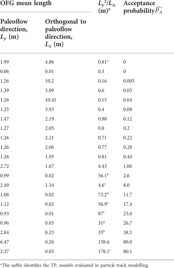
TABLE 1. Rate of producing plausible fields for 21 alternative geostatistical model hyperparameters, and the OFG mean lengths in the paleoflow (L_y) and perpendicular to paleoflow (L_x) directions. Representative samples from the range of plausible geostatistical model hyperparameters identified in the initial conditioning step were selected for prediction uncertainty analysis are identified by a suffix (a to i).

The following steps summarize this process of conditioning the TP models, using stochastic inversion (also depicted in Figure 3).

1. Generate empirical transiograms from the lithological logs at specified lags (Eq. 1).

2. Draw realizations from a prior hyperparameter distribution of the mean lengths in the paleoflow, transverse and vertical directions of the OFG lithological category.

3. Derive TP model based on the mean lengths, and the calculated textural class proportions from lithological logs for the same specified lags as in Eq. 1) above (Eqs 3a and 3b).

4. Compare modelled and empirical transition probabilities at specified lag distances (Eq. 4).

5. Adjust hyperparameter values using stochastic inversion algorithm until a good fit between modelled and measured transition probabilities is obtained.

6. Repeat the process until first and second moments of the distribution of mean OFG lengths have stabilized.

FIGURE 3

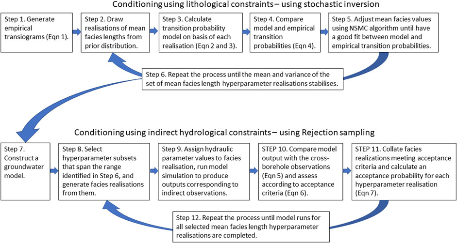
FIGURE 3. Flow chart showing the steps involved in the sequential Monte Carlo modelling procedure.

3.4 Conditioning using indirect hydrological constraints with rejection sampling

We adopted a straightforward implementation of rejection sampling, consistent with the Generalized likelihood uncertainty estimation (GLUE) method introduced by Beven & Binley (1992). It relies on generating multiple realizations from a prior probability distribution, running the model with each realization, and comparing model outputs with the observations. Each realization that does not provide a good fit to measured observations is rejected.

However, the ‘indirect’ nature of the observations of cross-borehole connectivity requires many additional steps before the information in these observations can be used to condition TP model hyperparameters. For every hyperparameter set we generate multiple aquifer heterogeneity realizations. Each realization is then converted to a hydraulic parameter field and used in a groundwater model simulation. Based on work in Dann et al. (2008 and 2009), this assignment of hydraulic conductivity values for OFG is 100 times that of the other three categories. The groundwater model simulates a flow process that provides outputs that correspond to the observations of cross-borehole connectivity. The details of this groundwater model are discussed in the following section.

Cross-borehole connectivity observations can be denoted as ${flux}_i$. When a model-to-measurement comparison is made, it is assessed according to an acceptance metric ${\varnothing }_{hydrology\left(\theta \right)}$which defines the sum of differences between the observed and modelled cross-borehole fluxes across all $n_{obs}$ observed fluxes, i.e. the sum of squared residuals or L2 norm:

${\varnothing }_{\mathit{h}\mathit{y}\mathit{d}\mathit{r}\mathit{o}\mathit{l}\mathit{o}\mathit{g}\mathit{y}\left(\mathit{\theta }\right)}={\sum }_{\mathit{i}=\mathbf{1}}^{{\mathit{n}}_{\mathit{o}\mathit{b}\mathit{s}}}{\left({\mathit{f}\mathit{l}\mathit{u}\mathit{x}}_{\mathit{i}}\left(\mathit{\theta }\right)-{\mathit{f}\mathit{l}\mathit{u}\mathit{x}}_{\mathit{i}}\right)}^{\mathbf{2}}(5)$

where $\theta$ defines the vector of hydraulic parameters defining the realization, which are generated from a specific geostatistical hyperparameter set and random seed. An acceptable fit threshold is applied to the fits between modelled and observed cross-borehole fluxes, defined as ${\varnothing }_{hydrology\left(\mathit{max}\right)}$. This is used to define a set of acceptable realizations, $\mathrm{\Omega }\left({\varnothing }_{hydrology\left(\theta \right)}\right)$ as:

$\mathrm{\Omega }\left({\varnothing }_{hydrology\left(\theta \right)}\right)=\{\begin{array}{c}0,{\varnothing }_{hydrology\left(\theta \right)}>{\varnothing }_{hydrology\left(\mathit{max}\right)}\\ 1,{\varnothing }_{hydrology\left(\theta \right)}\le {\varnothing }_{hydrology\left(\mathit{max}\right)}\end{array}(6)$

Note that this set will vary if the acceptance threshold is varied.

Collating the heterogeneity realizations that meet the acceptance threshold in Eq. 6 provides an acceptance probability $\widehat{P_A}$for each mean hydrofacies length hyperparameter set Eq. 7:

$\widehat{P_A}=\frac{1}{N_r}={\sum }_{i=1}^{N_r}\mathrm{\Omega }\left({\varnothing }_{hydrology\left(i\right)}\right)(7)$

where $N_r$ is the total number of realizations.

In summary, this rejection sampling process requires the generation of both hyperparameter realizations (also described as hyperparameter sets in the discussion that follows to avoid confusion with the aquifer heterogeneity realizations) as well as heterogeneity realizations and the hydraulic conductivity realizations based on them. The following steps summarize this process (as depicted in Figure 3):

7. Construct a groundwater flow model that simulates a flow field to represent the cross-borehole connectivity observations revealed by the smoke tracer test.

8. Select a subset of hyperparameter realizations that span the range of mean OFG length values defined in step 6 and generate an ensemble of heterogeneity realizations on the basis of each selected hyperparameter realization.

9. Assign hydraulic parameter values to the high and low conductivity categories of each realization, import these into the flow model, and run the flow model simulation to provide model outputs that correspond to cross-borehole observations.

10. Compare model outputs with these indirect observations (Eq. 5) and retain or reject the heterogeneity realization depending on whether the model-to-observation fit is sufficient to meet the selected acceptance criteria (Eq. 6).

11. Collate those heterogeneity realizations that meet the acceptance criteria and calculate an acceptance probability for each geostatistical model hyperparameter set.

12. For each of the selected subset of geostatistical hyperparameter realizations, return to Step 9 and continue until all realizations have been completed.

3.5 The flow model

Heterogeneity realizations were generated at a regular fine-scale grid discretization which covered the case study site (Step 8 above): an area of 40 m by 50 m by 10 m, with a grid cell dimension of 1 m by 1 m in the horizontal direction, and 0.1 m in the vertical direction. As noted above, each category (i.e. OFG and the combined SG, S and CBG category) was assigned a hydraulic conductivity value that represented the mean value for that category, transforming the heterogeneity realizations to hydraulic conductivity field realizations. Note that the cross-borehole flow observations are dependent on the relative hydraulic parameter values, rather than absolute hydraulic parameter values, and in this case the OFGs have a conductivity value that is three orders of magnitude higher than the other three textural classes.

Each hydraulic conductivity realization was used in a series of flow model simulations, implemented using the USGS software MODFLOW (Harbaugh et al., 2000), where cross-borehole connectivity observations derived from the smoke tracer test were modelled as being analogous to groundwater flow. The relative connectivity derived from the smoke tracer tests, was simulated using a steady-state flow field. In this flow field the boreholes were represented as constant head cells. For each of the smoke tracer experiments, the smoke injection borehole was assigned a positive head and remaining boreholes were assigned a zero head. No-flow boundaries were assigned around the edge of the model domain. The resulting pattern of cross-borehole flows was evaluated. This approach was possible because it was not necessary to simulate the smoke particle movement, as only the cross-borehole connectivity observations are used to screen out improbable heterogeneity structures in this study.

Using MODFLOW to simulate the flow of fluids other than groundwater, such as vapor transport in the unsaturated zone, relies on the analogies between these two flow problems (USEPA, 1995), and is appropriate where differential pressures are low, as demonstrated in Massmann (1989). This approach has also been used when simulating oil flows (Hsieh, 2011), when simulating multiphase flow in coal seam gas problems (Herckenrath et al., 2015), and can be used in advection-dispersion contexts (Rubbab et al., 2016).

Using this approach, three flow simulations were undertaken, representing each of the smoke injection bore tests depicted in Figure 2. This approach was both sufficient for simulation of the cross-borehole flow connectivity observations and provided a convenient and rapid-to-deploy surrogate for smoke transport simulation. Individual realizations were considered ‘plausible’ if the sum of the simulated head dependent discharges corresponding to the three most dominant connections, depicted in Figure 2, comprised 50% or more of the total discharge. The approximate and categorical nature of this acceptance criteria implicitly accounted for measurement and conceptual uncertainty that would impact on the precision of model to measurement fits and resembles Dorn et al. (2012) who used observations of the degree of fracture connectivity with similarly approximate acceptance criteria.

3.6 Assessment of prediction uncertainty using single and multiple plausible TP models

The implications of adopting a single geostatistical model are explored for simulations of groundwater transit times. The transit time prediction was simulated with a particle moving through a saturated steady-state flow field, with fixed head boundaries at opposite west and east sides of the model domain, and no flow boundaries at the north and south sides. The flow field was derived from a hydraulic property field relating to the aquifer heterogeneity realizations generated in the same manner as Step 9 above. These predictions were generated for 10 hyperparameter realizations which spanned the range of mean length hyperparameters identified with low to high acceptance criteria in the rejection sampling step. A total of 1,000 heterogeneity realizations were generated for each of the ten selected hyperparameter sets.

The groundwater model domain and hydraulic property values were the same as those used to simulate the cross-borehole connectivity observations described above. Constant head cells were placed at the upstream and downstream extent of the model domain. MODFLOW (Harbaugh et al., 2000) was used to simulate this groundwater flow field, and the transit time of the particle was simulated using the MODFLOW ADV package (Anderman & Hill, 2001). Transit time probability distributions for selected geostatistical model hyperparameter realizations were then explored.

4 Results and discussion

We examine and discuss the results of the numerical experiments from this study within a contaminant transport predictive context. Contaminant transport is very sensitive to the disposition of highly permeable pathways in aquifer systems (Lee et al., 2007; Fiori, & Jankovic, 2012; Soltanian & Ritzi, 2014; De Barros et al., 2016; Sanchez-Vila & Fernàndez-Garcia, 2016; Theel et al., 2020). This is particularly so for pathogen transport where risks are largely related to the fastest transit times through an aquifer, as pathogen numbers reduce over time at a rate governed by the half-life of the pathogen of concern (Hunt & Johnson, 2017).

Specifically, this section discusses the performance of the methodology used to condition the geostatistical model of OFG rapid transport pathways. The stochastic exploration of the ill-posed geostatistical model discussed in this section has similarities to the approaches described in Zhu et al. (2016), and Harp & Vesselinov (2012). This section also discusses the implications of the remaining geostatistical model uncertainty for pathogen transport predictions. The OFG lithological category controls how much and how quickly groundwater flows in our case study (Dann et al., 2009), and the geostatistical model hyperparameters correspond to the mean lengths of this category in the paleoflow direction (y or dip direction), transverse to this direction (x or strike direction), and the z-direction.

4.1 Sequential conditioning: Performance of initial stochastic inversion step

A total of 130 TP model hyperparameter realizations were generated from the stochastic inversion process, with the mean and standard deviations of the initial conditioning of the hyperparameter distribution having stabilized with this number of conditioned realizations. Each of the conditioned hyperparameter realizations resulted in modelled-to-measured transition probability fits with correlation coefficients of approximately 0.8. The standard deviations of the TP model hyperparameters (mean lengths of OFG in the paleoflow, transverse and vertical directions) were significantly reduced in this initial conditioning step from the reasonably unconstrained prior in the log domain of three log(m) in the x and y directions and one log(m) in the z-direction to 0.14 log(m) in the x-direction, 0.2 log(m) in the y-direction and 0.22 log(m) in the z-direction.

Despite the substantial reduction in the uncertainty achieved through the initial conditioning step, the remaining hyperparameter uncertainty can result in very different heterogeneity structures (Figure 4). For example, Figure 4 (upper part of Figure 4), shows two modelled-to-measured transiogram fits, where OFG mean lengths in the paleoflow y-direction (L_y) were 0.99 m for the left-hand side of the figure and 2.37 m on the right-hand side. A comparison of the heterogeneity realizations corresponding to these two hyperparameter sets (lower part of Figure 4) shows more elongated connected OFGs in the right-hand side of the plot, than those on the left.

FIGURE 4

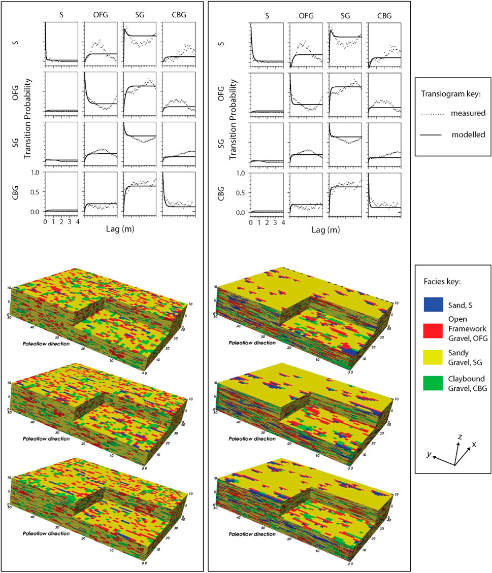
FIGURE 4. Modelled vertical transition probabilities (black line), and calculated transition probabilities from the lithological data (black dots) at the Kyle site for two statistically valid TP models are shown in the left and right columns. The left and right-hand columns correspond to suffix ‘b’, and ‘i’ in Table 1. Below the transiograms are three heterogeneity realizations relating to the TP models shown in the transiograms.

The non-uniqueness of the TP model hyperparameters, as depicted in Figure 4, reflects the lack of information regarding the OFG category mean lengths in the lateral direction (L_x). Non-uniqueness of geostatistical models is acknowledged and discussed in several studies (Harp & Vessilinov, 2012; Koch, 2013; He et al., 2014; Siena & Riva, 2020). Despite this, the impact of geostatistical model equifinality on the quantification of the uncertainty of groundwater model predictions of interest is seldom considered by practitioners in decision support models (Sanchez-Villa & Fernandez-Garcia, 2016). A component of the barrier to the uptake of stochastic methods relates to the computational burden of their implementation (Linde et al., 2015).

4.2 Sequential conditioning: Performance of rejection sampling step

A selection of 21 hyperparameter sets were selected so that they spanned the OFG hyperparameter range identified in the first conditioning step. Details of these 21 hyperparameter sets are listed in Table 1. Heterogeneity realizations were then generated, with more than 17,000 heterogeneity realizations being generated for each of the selected hyperparameter sets. Each realization was then used in a flow simulation of cross-borehole connectivity. The proportion of flow simulations, associated with each heterogeneity realization, that met the cross-borehole connectivity acceptance criteria ranged from 0 to 81%. This approach of ranking the plausibility of TP model hyperparameter sets using a system response-based acceptance criteria was also used by Harp & Vesselinov (2010) and Dorn et al. (2012), when conditioning geostatistical facies and fracture network models respectively.

Examination of the relationship between acceptance probabilities and the disposition of the OFG provided important information. The range of the mean vertical thickness (L_z) of the OFG category was reasonably well constrained on the basis of the lithological data, and varied from 0.13 m to 0.43 m, with an average of 0.23 m. These small variations in these OFG thicknesses did not impact on the plausibility of hyperparameter sets, whereas the lateral (L_y) and transverse (L_x) OFG dimensions did.

Figure 5 shows the relationship between OFG category mean lengths and acceptance probabilities, expressed using a ratio of the squared mean length in the paleoflow y-direction (L_y) and the x-direction (L_x). The ratio between L_y and L_x can convey the relationship between the relative mean lengths in the x and y-directions, whereas the absolute magnitude of the mean length is incorporated into the ratio by squaring the L_y term. By ranking the mean OFG dimensions by their propensity to produce realizations which generate model outputs that are consistent with the indirect observations, additional information is provided about the spatial disposition of the OFGs.

Various relationships between acceptance probability and the mean length hyperparameters were analyzed to explore this information. The absolute magnitude of these ratios was found to be important when simulating the cross-borehole flows, correlating strongly with acceptance probabilities. Long and narrow OFGs, elongated in the paleoflow direction, were found to be positively correlated with higher acceptance probabilities (Figure 5; Table 1). In contrast, small OFG lengths in the paleoflow direction, or large OFG widths (direction orthogonal to paleoflow), had very low acceptance probabilities.

Table 1 lists the OFG mean lengths in the paleoflow direction, (L_y), and orthogonal to this direction, (L_x), for the 21 selected hyperparameter sets. It also lists the L_y²/L_x ratio and acceptance probabilities, ($\widehat{P_A}$) for the 21 selected hyperparameter sets, which are also depicted in Figure 5. Of the realizations summarized in Table 1, two different geostatistical models achieved the highest acceptance probability of 80%; these occurred for the models which had a L_y²/L_x ratio of 178 and 158.6. These ratios corresponded to mean lengths between 2.37 m and 6.47 m in the paleoflow y-direction (L_y) and mean widths of 0.03 m–0.26 m in the x-direction (L_x). These acceptance probability figures indicate that the lack of OFG connectivity in the direction orthogonal to paleoflow (x-direction) was as important as the connectivity in the paleoflow y-direction when reproducing the cross-borehole connectivity observations. This strongly directional dependent nature of the OFG connectivity was not indicated by the lithological logs alone. Some of the other TP models listed in Table 1, while not producing such high acceptance probabilities, still provided some realizations which meet the acceptance criteria. Therefore, those geostatistical model hyperparameter sets cannot be discounted as valid.

The overall greater connectivity of the OFG in the paleoflow direction across the range of hyperparameters explored is depicted in probability plots as shown in Figure 6. Figure 6A shows the probability of OFGs occurring for all selected TP models, denoted ‘a’ to ‘i’ in Table 1, spanning the range of acceptance probabilities from 0 to 80%. A probability of one occurs where OFGs were observed directly in the lithological logs, as depicted in Figures 6A and 6B, with probabilities approaching one clustered around borehole locations. With greater distance from the boreholes, these probabilities gradually reduce to background levels of 0.14, representing the bulk proportion of OFGs at this site.

FIGURE 6

FIGURE 6. OFG probability models showing the spatial probability of OFGs occurring at a probability of greater than 0.25: (A) for combined realizations from TP models labelled ‘a’ to ‘I’ in Table 1; and (B) for realizations from a single TP model labelled a0 in Table 1.

Figure 6B depicts the probability of OFGs occurring in any model cell, for a single TP model (denoted as ‘a’ in Table 1) which corresponds to an acceptance probability of zero. Figure 6B depicts wider OFGs in the direction orthogonal to the paleoflow direction. These wider OFG’s would tend to allow greater cross-bore connectivity orthogonal to the paleoflow direction, which is inconsistent with the smoke tracer test observations.

Harter (2005), Fogg et al. (2000), and Fogg & Zhang (2016) discuss how the upper 12–28% of a hydraulic conductivity distribution will tend to be fully connected in 3-D created random fields. This proportional range of high conductivity facies encompasses the bulk proportion of OFGs in this study. Fogg & Zhang (2016) assert that this connectivity will lead to laterally and vertically extensive rapid transport pathways. The OFG probabilities shown in Figure 6A provide an indication of the disposition of such connected pathways.

4.3 Sequential conditioning summary

The sequential conditioning approach adopted, combining stochastic inversion and rejection sampling was able to support the conditioning to direct and indirect geological observations. Rejection sampling revealed the anisotropy of the OFGs more fully and was required only when conditioning to the cross-bore flow observations, to adhere to the conceptual model for geologic heterogeneity. Many more model runs would have been required if rejection sampling had been applied as part of a joint inversion approach. This study provides a demonstration of using a sequential conditioning approach comprised of two history matching methods to successfully negotiate the pitfalls of numerical inefficiency on one hand and degradation of the geological model on the other.

4.4 Implications of geostatistical model equifinality for contaminant risk assessments

Particle tracking simulations are often used to assess the risks associated with rapid transport rates of pathogens in groundwater (Hunt & Johnson, 2017). We adopted this approach when assessing the impact on transit time predictions incurred by adopting a single geostatistical model. In total, 1,000 realizations were used from selected geostatistical models (identified as (a) to (i) in Table 1). This subset of nine out of 21 hyperparameters sets explored were selected to span the range of acceptance probabilities identified.

The distribution of particle paths simulated on the basis of each realization, that were generated from the nine selected TP model hyperparameter sets, are mapped in plan-view in Figure 7. The corresponding acceptance probability listed in Table 1 is also noted in Figure 7 for each model, with model (i) having the highest acceptance probability of 80%. Blue particle paths correspond to all realizations generated for each hyperparameter set, while red particle paths correspond to only those realizations which met the cross-borehole acceptance criteria. Figure 7 shows particle tracks have less lateral spread and are more closely aligned with the groundwater flow direction for those models associated with higher acceptance probabilities. This is consistent with the narrow and longer disposition of OFG pathways identified through conditioning to the cross-borehole connectivity observations.

FIGURE 7

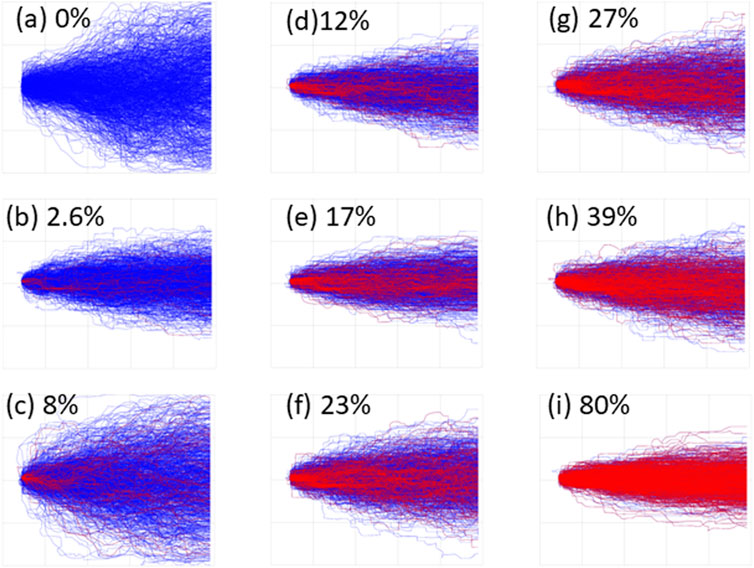
FIGURE 7. Particle tracks for selected TP models (a–i) are shown in blue. Particle tracks for plausible realizations for each model are shown in red. The acceptance probability for each of the figures are shown alongside the relevant model label.

The transit times corresponding to the particle tracks shown in Figure 7 were collated and are summarized in the box and whisker plot of Figure 8. Note that these times are normalized by using a porosity value that scales the maximum travel times for hyperparameter set (i) to be approximately 1 day, allowing the relativity of these travel times to be depicted rather than their absolute magnitude. For example, the hyperparameter set (c) results in a maximum travel time that is 500% greater than that of the hyperparameter set (i). The hyperparameter set (i) in the bottom right of Figure 8 provides the fastest particle travel times, and also provides the highest acceptance probability.

FIGURE 8

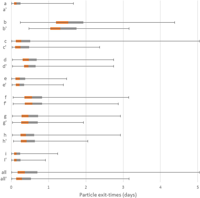
FIGURE 8. Box and whisker plots showing relative particle exit-times for TP models (a–i) together with their combined times (all). The ‘suffix represents the exit-times derived from the plausible realizations for each TP model. Box and whiskers represent the minimum, maximum and lower and upper quartile of the particle exit-times.

A comparison of the results from the other eight hyperparameter sets (a to h), is illuminating. It shows that particle transit times which met the cross-borehole acceptance criteria can fall well outside the range defined by the hyperparameter set (i) which had the highest acceptance probability. This has implications for analysis of predictive uncertainty. An analysis of transit time based on a single geostatistical model hyperparameter set with the highest acceptance probability, could significantly under-estimate the transit time uncertainty. Instead, a robust uncertainty analysis may need to consider predictions simulated from realizations generated from TP model hyperparameter sets with lower and higher acceptance probabilities. Therefore, while conditioning can reduce geostatistical model uncertainty, the results indicate that multiple plausible geostatistical models need to be considered for a prediction of concern in decision support modelling. This issue was also raised in Harp & Vessilinov (2012) when examining the quantification of the uncertainty of aquifer drawdown predictions.

This has practical implications for model-based risk assessments, and highlights the importance of considering the specific prediction being made when selecting geostatistical models. For this case study, when simulating pathogen contamination risks, the greatest risks would be exposed using model hyperparameter set (i), and would not have been exposed using model (b). If instead the concern had been related to inefficient use of land, due to over estimation of source protection zone areas, the greatest risk would be exposed by adopting model hyperparameter sets (b) or (f).

4.5 Additional considerations

In other prediction uncertainty studies based on TP geostatistical models, it may be important to also represent the variability of hydraulic properties within a defined category. Riva et al. (2006) found that representing hydraulic conductivity variability within a category could led to elongated capture zones, where this variability was being used to represent small-scale preferred flow paths. In contrast, Copty & Findikakis (2002) found that internal variability of hydraulic conductivity within defined categories had no significant impact on the predictions of a solute particle transport.

Those two studies exemplify the fact that any requirements for representing inter-category variability are context specific. Where realizations have been generated at significantly larger scales than the hydraulic property variability occurs, the geostatistical model is upscaled, and hence inter-category variability may be required if the prediction is sensitive to this variability. The study reported here sought to represent the fine scale detail of the permeable connected OFG category, populating a very fine model grid to explicitly represent preferred pathways. Therefore, the need to represent inter category variability was avoided in this study.

The 1 m by 1 m grid discretization used in this study required only slight upscaling of the transition probabilities in the x-direction, perpendicular to the paleoflow direction. The stochastic nature of prediction specific heterogeneity at field scales was not addressed in this study and remains a research challenge (Fogg et al., 2000; Fogg & Zhang, 2016; Doherty & Moore, 2019). Initial explorations into this field of research include hierarchical nested model frameworks (Li et al., 2006; Sreekanth & Moore, 2018), or the hybrid multiscale methods outlined in Scheibe et al. (2015). Local and global upscaling approaches can be used to derive the field scale versions of these stochastic models of aquifer heterogeneity if a robust fine-scale characterization of the heterogeneity exists (Fengjun et al., 2003; Chen, 2009; Zhou et al., 2010; Li et al., 2015; Soltanian et al., 2015; Li & Durlofsky, 2016).

5 Conclusion

Groundwater model predictions of contaminant transport, particularly pathogen contaminants, are sensitive to small-scale high permeability pathways. The ability to improve the characterization of geostatistical models that are used to describe these rapid transport pathway distributions is central to improving models used for water management decision support. However, the extent to which uncertainties in geostatistical models can influence the outcomes of a contaminant transport risk assessment is not well understood and is typically neglected in modelling practice.

In this study we have put considerable effort into conditioning geostatistical model hyperparameters and exploring their uncertainty, but it is common practice to adopt a single geostatistical model parameterization. We demonstrate that the selection of a single geostatistical model, without consideration of its relevance to the predictions that matter, may prevent the simulation of real predictive possibilities, undermining the quantification of risks. Risk based assessments may need to consider alternative geostatistical models in the context of particular types of predictions (e.g. predictions dependent on time of travel) to guarantee robust decision support.

Conditioning with both direct and indirect aquifer information can mitigate the impact of sparse geological data, allowing the uncertainty of geostatistical models to be significantly reduced. In this study the detailed lithological study documented in Burbery et al. (2017) supplemented by the observations of cross-borehole connectivity from smoke tracer tests, enabled geostatistical models of the risk salient aspects of OFG pathways in alluvial gravels to be defined i.e. the connectivity of the OFG rapid transport pathways. To the best of our knowledge, no studies combining fine detailed lithological logs from alluvial deposits with in-situ measurements of the connectivity of rapid transport pathways, have previously been used to derive a geostatistical model of small-scale high permeability groundwater pathways. The fine-scale characterization of highly permeable OFG pathway structure, made accessible by this study, provides a much-needed basis for the assessments of risk in these contexts.

The significant computational burden involved when conditioning geostatistical models with direct and indirect data is made more challenging if efficient conditioning methods risk degrading the geological realism of the geostatistical model. To address this, we developed a sequential conditioning approach that combines alternative history matching methods. This approach enables each dataset to be conditioned with the history matching method best suited to that data. Datasets that involve more processing are scheduled for processing in later steps, thereby supporting better management of the computational load.

This work also provides a basis for future research. The fine-scale characterization made accessible by this study provides a much-needed basis for the analysis of upscaled hydraulic parameters to field scales that account for the presence of OFG pathways when assessing the risk of early arrival times of pathogen contaminants. With better characterization of geostatistical models of rapid transport pathways, we can more reliably model groundwater flow and contaminant transport and provide improved environmental decision support at a range of scales.

The particle tracking predictive scenario discussed in this paper demonstrates the implications of the geostatistical model uncertainty in one specific predictive context. Future research may also explore an advection-dispersion transport predictive simulation to assess the implications of geostatistical model uncertainty for transport predictions that are more affected by factors such as dispersion or chemical reactions.

In summary, the results of this study illustrate the importance of considering geostatistical uncertainty, in the context of specific predictions. Adoption of a single geostatistical model can result in realistic predictions being overlooked. Prediction specific geostatistical models need to be selected, such as those of rapid transport pathways explored in this study, to ensure robust assessments of risk. Combining acceptable realizations from multiple credible geostatistical models, to ensure that the true predictive uncertainty range is conveyed, may be required. Alternatively, selection of a worse-case geostatistical model for a particular prediction could be adopted. This has important practical implications for uncertainty quantification and history matching when using ensemble-based methods, which are based on geostatistical models to generate prior parameter distributions.

Data availability statement

The raw data supporting the conclusion of this article will be made available by the authors, without undue reservation.

Author contributions

CM was the primary author of this article, with all co-authors also contributing to the manuscript. CM and DS undertook the numerical experiments documented in the paper. The ideas and concepts in the manuscript were co-developed principally by CM and DS with contributions from LB and MC. The case study details were all supplied by LB. The original concept and funding for this work was secured by MC. All authors have seen and approved the final version of the manuscript being submitted. They warrant that the article is the authors’ original work, has not received prior publication and is not under consideration for publication elsewhere.

Acknowledgments

This paper represents a collaboration between ESR and GNS Science, both in New Zealand, and was funded by the New Zealand Ministry of Business Innovation and Employment (grant nos. C03X1001 and C05X1803, and was also supported by GNS Science Groundwater Strategic Science Investment Fund (SSIF)).

Conflict of interest

The authors declare that the research was conducted in the absence of any commercial or financial relationships that could be construed as a potential conflict of interest.

Publisher’s note

All claims expressed in this article are solely those of the authors and do not necessarily represent those of their affiliated organizations, or those of the publisher, the editors and the reviewers. Any product that may be evaluated in this article, or claim that may be made by its manufacturer, is not guaranteed or endorsed by the publisher.

References

Alsharhan, A. S., and Rizk, Z. E. (2020). “Gravel aquifers,” in Water resources and integrated management of the United Arab Emirates (Cham: Springer), Vol. 3. doi:10.1007/978-3-030-31684-6_11

CrossRef Full Text | Google Scholar

Anderman, E. R., and Hill, M. C. (2001). MODFLOW-2000: The U.S. Geological survey modular ground-water model -- documentation of the advective-transport observation (ADV2) package, version 2: U.S, 54. Geological Survey Open-File Report, 69. doi:10.3133/ofr0154

CrossRef Full Text | Google Scholar

Ashworth, P., Best, J. L., Peakall, J., and Lorsong, J. A. (1999). “The influence of aggradation on braided alluvial architecture: Field study and physical scale modelling of the ashburton gravels, Canterbury plains, New Zealand,” in Fluvial sedimentology VI. Editors N. D. Smith, and J. Rogers (Special Publication of International Association of Sedimentologists), 28, 333–346.

Google Scholar

Bal, A. A. (1996). Valley fills and coastal cliffs buried beneath an alluvial plain: Evidence from variation of permeabilities in gravel aquifers, Canterbury plains, New Zealand. J. Hydrology (New Zealand) 35 (1), 1–27.

Google Scholar

Beven, K. J., and Binley, A. M. (1992). The future of distributed models: Model calibration and uncertainty prediction. Hydrol. Process. 6, 279–298. doi:10.1002/hyp.3360060305

CrossRef Full Text | Google Scholar

Bridge, J. S., and Lunt, I. A. (2006). “Depositional models of braided rivers,” in Braided rivers: Process, deposits, ecology and management. Editors G. S. Sambrook-Smith, J. L. Best, C. S. Bristow, and G. E. Petts (Oxford: Blackwell), 11–49. doi:10.1002/9781444304374.ch2

CrossRef Full Text | Google Scholar

Brown, L. J. (2001). “Canterbury,”. Groundwaters of New Zealand. Editors M. R. Rosen, and P. A. White (Wellington: The New Zealand Hydrological Society), 441–459.

Google Scholar

Browne, G. H., and Naish, T. R. (2003). Facies development and sequence architecture of a late quaternary fluvial-marine transition, Canterbury plains and shelf, New Zealand: Implications for forced regressive deposits. Sediment. Geol. 158 (1-2), 57–86. doi:10.1016/S0037-0738(02)00258-0

CrossRef Full Text | Google Scholar

Burbery, L. F., Jones, M. A., Moore, C. R., Abraham, P., Humphries, B., and Close, M. E. (2017). “Study of connectivity of open framework gravel facies in the Canterbury Plains aquifer using smoke as a tracer,” in Geology and geomorphology of alluvial and fluvial fans: Terrestrial and planetary perspectives (London: Geological Society). doi:10.1144/SP440.10

CrossRef Full Text | Google Scholar

Carle, S. F., and Fogg, G. E. (2020). Integration of soft data into geostatistical simulation of categorical variables. Front. Earth Sci. 8. doi:10.3389/feart.2020.565707

CrossRef Full Text | Google Scholar

Carle, S. F., and Fogg, G. E. (1997). Modeling spatial variability with one and multidimensional continuous-lag Markov chains. Math. Geol. 29 (7), 891–918. doi:10.1023/a:1022303706942

CrossRef Full Text | Google Scholar

Carle, S. (1999). T-PROGS: Transition probability geostatistical software. Davis: University of California. http://gmsdocs.aquaveo.com/t-progs.pdf.

Google Scholar

Cary, A. S. (1951). Origin and significance of openwork gravel. Trans. Am. Soc. Civ. Eng. 116 (1), 1296–1308. doi:10.1061/TACEAT.0006486

CrossRef Full Text | Google Scholar

Chan, S., and Elsheikh, A. H. (2020). Parametrization of stochastic inputs using generative adversarial networks with application in geology. Front. Water 2, 5. doi:10.3389/frwa.2020.00005

CrossRef Full Text | Google Scholar

Chen, T. (2009). New methods for accurate upscaling with full-tensor effects. PhD thesis, Energy and Resources Engineering, Stanford University. Available at https://pangea.stanford.edu/ERE/pdf/pereports/PhD/Chen09.pdf.

Google Scholar

Ciriello, V., Di Federico, V., Riva, M., Cadini, F., de Sanctis, J., Zio, E., et al. (2013). Polynomial chaos expansion for global sensitivity analysis applied to a model of radionuclide migration in a randomly heterogeneous aquifer. Stoch. Environ. Res. Risk Assess. 27, 945–954. doi:10.1007/s00477-012-0616-7

CrossRef Full Text | Google Scholar

Cirpka, O. A., and Valocchi, A. J. (2016). Debates—stochastic subsurface hydrology from theory to practice: Does stochastic subsurface hydrology help solving practical problems of contaminant hydrogeology? Water Resour. Res. 52 (12), 9218–9227. doi:10.1002/2016WR019087

CrossRef Full Text | Google Scholar

Copty, N. K., and Findikakis, A. N. (2002). Uncertainty analysis of a well capture zone under multiple scales of heterogeneity. in “Calibration and reliability in groundwater modelling: A few steps closer to reality: Proceedings of ModelCARE'2002”. Prague, Czech Republic: IAHS Publ.

Google Scholar

Dann, R., Close, M. E., Flintoft, M. J., Hector, R., Barlow, H., Thomas, S., et al. (2009). Characterization and estimation of hydraulic properties in an alluvial gravel vadose zone. Vadose Zone J. 8 (3), 651–663. doi:10.2136/vzj2008.0174

CrossRef Full Text | Google Scholar

Dann, R., Close, M. E., Pang, L., Flintoft, M. J., and Hector, R. (2008). Complementary use of tracer and pumping tests to characterize a heterogeneous channelized aquifer system in New Zealand. Hydrogeol. J. 16, 1177–1191. doi:10.1007/s10040-008-0291-4

CrossRef Full Text | Google Scholar

De Barros, F. P. J., Bellin, A., Cvetkovic, V., Dagan, G., and Fiori, A. (2016). Aquifer heterogeneity controls on adverse human health effects and the concept of the hazard attenuation factor. Water Resour. Res. 52 (8), 5911–5922. doi:10.1002/2016wr018933

CrossRef Full Text | Google Scholar

De Luca, D. A., Lasagna, M., and Debernardi, L. (2020). Hydrogeology of the Western Po plain (piedmont, NW Italy). J. Maps 16 (2), 265–273. doi:10.1080/17445647.2020.1738280

CrossRef Full Text | Google Scholar

Deutsch, C. V., and Journel, A. G. (1998). Geostatistical software library and user’s guide. 2nd Edn. New York, NY: Oxford University Press.

Google Scholar

Deutsch, C. V., and Tran, T. T. (2002). Fluvsim: A program for object-based stochastic modeling of fluvial depositional systems. Comput. Geosciences 28 (4), 525–535. doi:10.1016/S0098-3004(01)00075-9

CrossRef Full Text | Google Scholar

Doherty, J. (2015). Calibration and uncertainty analysis for complex environmental models. Brisbane, Australia: Watermark Numerical Computing.

Google Scholar

Doherty, J., and Moore, C. (2021). “Decision support modelling viewed through the lens of model complexity,” in A GMDSI monograph (South Australia: National Centre for Groundwater Research and Training, Flinders University). doi:10.25957/p25g-0f58

CrossRef Full Text | Google Scholar

Doherty, J., and Moore, C. R. (2019). Decision support modeling: Data assimilation, uncertainty quantification, and strategic abstraction. Groundwater 58 (3), 327–337. doi:10.1111/gwat.12969

PubMed Abstract | CrossRef Full Text | Google Scholar

Doherty, J. (2016). User’s manual for PEST version 14.2. Brisbane, Queensland, Australia: Watermark Numerical Computing, 339.

Google Scholar

Dorn, C., Linde, N., Le Borgne, T., Bour, O., and Klepikova, M. (2012). Inferring transport characteristics in a fractured rock aquifer by combining single-hole ground-penetrating radar reflection monitoring and tracer test data. Water Resour. Res. 48, W11521. doi:10.1029/2011WR011739

CrossRef Full Text | Google Scholar

Engdahl, N. B., and Weissmann, G. S. (2010). Anisotropic transport rates in heterogeneous porous media. Water Resour. Res. 46, W02507. doi:10.1029/2009WR007910

CrossRef Full Text | Google Scholar

Fengjun, Z., Reynolds, A. C., and Oliver, D. S. (2003). The impact of upscaling errors on conditioning a stochastic channel to pressure data. SPE J. 8, 13–21. doi:10.2118/83679-PA

CrossRef Full Text | Google Scholar

Ferreira, J. T., Ritzi, R. W., and Dominic, D. F. (2010). Measuring the permeability of open-framework gravel. Ground Water 48 (4), 593–597. doi:10.1111/j.1745-6584.2010.00675.x

PubMed Abstract | CrossRef Full Text | Google Scholar

Feyen, L., Gómez-Hernández, J. J., Ribeiro, P. J., Beven, K. J., and De Smedt, F. (2003). A Bayesian approach to stochastic capture zone delineation incorporating tracer arrival times, conductivity measurements, and hydraulic head observations. Water Resour. Res. 39 (5). doi:10.1029/2002WR001544

CrossRef Full Text | Google Scholar

Fiori, A., Dagan, G., Jankovic, I., and Zarlenga, A. (2013). The plume spreading in the MADE transport experiment: Could it be predicted by stochastic models? Water Resour. Res. 49, 2497–2507. doi:10.1002/wrcr.20128

CrossRef Full Text | Google Scholar

Fiori, A., and Jankovic, I. (2012). On preferential flow, channeling and connectivity in heterogeneous porous formations. Math. Geosci. 44 (2), 133–145. doi:10.1007/s11004-011-9365-2

CrossRef Full Text | Google Scholar

Flynn, R. M., Mallen, G., Engel, M., Ahmed, A., and Rossi, P. (2015). Characterizing aquifer heterogeneity using bacterial and bacteriophage tracers. J. Environ. Qual. 44 (5), 1448–1458. doi:10.2134/jeq2015.02.0117

PubMed Abstract | CrossRef Full Text | Google Scholar

Fogg, G. E., Carle, S. F., and Green, C. (2000). “A connected-network paradigm for the alluvial aquifer system,” in Theory, modelling and field investigation in hydrogeology: A special volume in honor of shlomo P. Neuman’s 60th birthday, GSA special paper 348. Editors D. Zhang, and C. L. Winter (Boulder, CO: Geological Society of America), 348, 25–42.

CrossRef Full Text | Google Scholar

Fogg, G. E., and Zhang, Y. (2016). Debates—stochastic subsurface hydrology from theory to practice: A geologic perspective. Water Resour. Res. 52, 9235–9245. doi:10.1002/2016WR019699

CrossRef Full Text | Google Scholar

Gilpin, B. J., Walker, T., Paine, S., Sherwood, J., Mackereth, G., Wood, T., et al. (2020). A large scale waterborne Campylobacteriosis outbreak, Havelock North, New Zealand. J. Infect. 81 (3), 390–395. doi:10.1016/j.jinf.2020.06.065

PubMed Abstract | CrossRef Full Text | Google Scholar

Goovaerts, P. (1997). “Geostatistics for natural resources evaluation,” in Applied geostatistics series (New York, NY: Oxford University Press).

Google Scholar

Government Inquiry into Havelock North Drinking Water (2017). Report of the Havelock North drinking water Inquiry: Stage 1. Available at https://www.dia.govt.nz/Stage-1-of-the-Water-Inquiry.

Google Scholar

Hansen, A. L., Gunderman, D., He, X., and Refsgaard, J. (2014). Uncertainty assessment of spatially distributed nitrate reduction potential in groundwater using multiple geological realizations. J. Hydrology 519, 225–237. doi:10.1016/j.jhydrol.2014.07.013

CrossRef Full Text | Google Scholar

Harbaugh, A. W., Banta, E. R., Hill, M. C., and McDonald, M. G., (2000). MODFLOW-2000: The U.S. Geological survey modular ground-water model – user guide to modularization concepts and the ground-water flow process. U.S Geological Survey Open-File, 121. doi:10.3133/ofr200092

CrossRef Full Text | Google Scholar

Harp, D., Dai, Z., Wolfsberg, A., Vrugt, J., Robinson, B., and Vesselinov, V. (2008). Aquifer structure identification using stochastic inversion. Geophys. Res. Lett. 35, L08404. doi:10.1029/2008GL033585

CrossRef Full Text | Google Scholar

Harp, D. H., and Vesselinov, V. V. (2012). Analysis of hydrogeological structure uncertainty by estimation of hydrogeological acceptance probability of geostatistical models. Adv. Water Resour. 36, 64–74. doi:10.1016/j.advwatres.2011.06.007

CrossRef Full Text | Google Scholar

Harp, D. H., and Vesselinov, V. V. (2010). Stochastic inverse method for estimation of geostatistical representation of hydrogeologic stratigraphy using borehole logs and pressure observations. Stoch. Environ. Res. Risk Assess. 24 (7), 1023–1042. doi:10.1007/S00477-010-0403-2

CrossRef Full Text | Google Scholar

Harter, T. (2005). Finite-size scaling analysis of percolation in three-dimensional correlated binary Markov chain random fields. Phys. Rev. E 72 (2), 026120. doi:10.1103/PhysRevE.72.026120

PubMed Abstract | CrossRef Full Text | Google Scholar

Hassan, A., Bekhit, H., and Chapman, J. (2009). Using Markov chain Monte Carlo to quantify parameter uncertainty and its effect on predictions of a groundwater flow model. Environ. Model. Softw. (24), 749–763. doi:10.1016/j.envsoft.2008.11.002

CrossRef Full Text | Google Scholar

He, X., Koch, J., Sonnenborg, T. O., Jorgensen, F., Schamper, C., and Refsgaard, J. C. (2014). Transition probability-based stochastic geological modeling using airborne geophysical data and borehole data. Water Resour. Res. 50, 3147–3169. doi:10.1002/2013WR014593

CrossRef Full Text | Google Scholar

Herckenrath, D., Doherty, J., and Panday, S. (2015). Incorporating the effect of gas in modelling the impact of CBM extraction on regional groundwater systems. J. Hydrology 523 (3–4), 587–601. doi:10.1016/j.jhydrol.2015.02.012

CrossRef Full Text | Google Scholar

Hsieh, P. A. (2011). Application of MODFLOW for oil reservoir simulation during the deepwater horizon crisis. Ground Water 49 (3), 319–323. doi:10.1111/j.1745-6584.2011.00813.x

PubMed Abstract | CrossRef Full Text | Google Scholar

Huang, X., Li, J., Liang, Y., Wang, Z., Guo, J., and Jiao, P. (2017). Spatial hidden Markov chain models for estimation of petroleum reservoir categorical variables. J. Pet. Explor. Prod. Technol. 7, 11–22. doi:10.1007/s13202-016-0251-9

CrossRef Full Text | Google Scholar

Hunt, R. J., and Johnson, W. P. (2017). Pathogen transport in groundwater systems: Contrasts with traditional solute transport. Hydrogeol. J. 25, 921–930. doi:10.1007/s10040-016-1502-z

CrossRef Full Text | Google Scholar

Huysmans, M., and Dassargues, A. (2009). Application of multiple-point geostatistics on modelling groundwater flow and transport in a cross-bedded aquifer (Belgium). Hydrogeol. J. 17, 1901–1911. doi:10.1007/s10040-009-0495-2

CrossRef Full Text | Google Scholar

Jafarpour, B., and Tarrahi, M. (2011). Assehe performance of the ensemble Kalman filter for subsurface flow data integration under variogram uncertainty. Water Resour. Res. 47 (5), W05537. doi:10.1029/2010WR009090

CrossRef Full Text | Google Scholar

Jussel, P., Stauffer, F., and Dracos, T. (1994). Transport modeling in heterogeneous aquifers: 1. Statistical description and numerical generation of gravel deposits. Water Resour. Res. 30, 1803–1817. doi:10.1029/94WR00162

CrossRef Full Text | Google Scholar

Kennedy, M. C., and O'Hagan, A. (2002). Bayesian calibration of computer models. J. R. Stat. Soc. B 63, 425–464. doi:10.1111/1467-9868.00294

CrossRef Full Text | Google Scholar

Klingbeil, R., Kleineidam, S., Asprion, U., Aigner, T., and Teutsch, G. (1999). Relating lithofacies to hydrofacies: Outcrop-based hydrogeological characterisation of quaternary gravel deposits. Sediment. Geol. 129 (3), 299–310. doi:10.1016/S0037-0738(99)00067-6

CrossRef Full Text | Google Scholar

Koch, J. (2013). “Geological heterogeneity in the Norsminde catchment – a hydrogeological perspective,” Master’s thesis: University of Copenhagen.

Google Scholar

Koltermann, C. E., and Gorelick, S. M. (1996). Heterogeneity in sedimentary deposits: A review of structure-imitating, process-imitating, and descriptive approaches. Water Resour. Res. 32 (9), 2617–2658. doi:10.1029/96WR00025

CrossRef Full Text | Google Scholar

Leckie, D. A. (1994). Canterbury Plains, New Zealand: Implications for sequence stratigraphic models. Am. Assoc. Pet. Geol. Bull. 78 (8), 1240–1256. doi:10.1306/A25FEABD-171B-11D7-8645000102C1865D

CrossRef Full Text | Google Scholar

Leckie, D. A. (2003). Modern environments of the Canterbury plains and adjacent offshore areas, New Zealand — An analog for ancient conglomeratic depositional systems in nonmarine and coastal zone settings. Bull. Can. Petroleum Geol. 51 (4), 389–425. doi:10.2113/51.4.389

CrossRef Full Text | Google Scholar

Lee, S-Y., Carle, S. F., and Fogg, G. E. (2007). Geologic heterogeneity and a comparison of two geostatistical models: Sequential Gaussian and transition probability-based geostatistical simulation. Adv. Water Resour. 30, 1914–1932. doi:10.1016/j.advwatres.2007.03.005

CrossRef Full Text | Google Scholar

Li, H., and Durlofsky, L. J. (2016). Local–global upscaling for compositional subsurface flow simulation. Transp. Porous Med. 111, 701–730. doi:10.1007/s11242-015-0621-7

CrossRef Full Text | Google Scholar

Li, J., Lei, Z., Qin, G., and Gong, B. (2015). Effective local-global upscaling of fractured reservoirs under discrete fractured discretization. Energies 8, 10178–10197. doi:10.3390/en80910178

CrossRef Full Text | Google Scholar

Li, S.-G., Liu, Q., and Afshari, S. (2006). An object-oriented hierarchical patch dynamics paradigm (HPDP) for modeling complex groundwater systems across multiple-scales. Environ. Model. Softw. 21 (5), 744–749. doi:10.1016/j.envsoft.2005.11.001

CrossRef Full Text | Google Scholar

Li, W., and Zhang, C. (2019). Markov chain random fields in the perspective of spatial Bayesian networks and optimal neighborhoods for simulation of categorical fields. Comput. Geosci. 23, 1087–1106. doi:10.1007/s10596-019-09874-z

CrossRef Full Text | Google Scholar

Linde, N., Renard, P., Mukerji, T., and Caers, J. (2015). Geological realism in hydrogeological and geophysical inverse modeling: A review. Adv. Water Resour. 86, 86–101. doi:10.1016/j.advwatres.2015.09.019

CrossRef Full Text | Google Scholar

Lunt, I. A., and Bridge, J. S. (2007). Formation and preservation of open-framework gravel strata in unidirectional flows. Sedimentology 54 (1), 71–87. doi:10.1111/j.1365-3091.2006.00829.x

CrossRef Full Text | Google Scholar

Lunt, I. A., Bridge, J. S., and Tye, R. S. (2004). “Development of a 3D depositional model of braided river deposits,”. in “Aquifer characterization” Editors J. S. Bridge, and D. W. Hyndman (Society for Sedimentary Geology, Special Publications), 80, 39–169. doi:10.2110/pec.04.80.0139

CrossRef Full Text | Google Scholar

Massmann, J. W. (1989). Applying groundwater flow models in vapor extraction system design. J. Environ. Eng. New. York. 115, 129–149. doi:10.1061/(asce)0733-9372(1989)115:1(129)

CrossRef Full Text | Google Scholar

Oliveira, G. S., Soares, A. O., Schiozer, D. J., and Maschio, C. (2017). Reducing uncertainty in reservoir parameters combining history matching and conditioned geostatistical realizations. J. Petroleum Sci. Eng. 156, 75–90. doi:10.1016/j.petrol.2017.05.003

CrossRef Full Text | Google Scholar

Pang, L. (2009). Microbial removal rates in subsurface media estimated from published studies of field experiments and large intact soil cores. J. Environ. Qual. 38 (4), 1531–1559. doi:10.2134/jeq2008.0379

PubMed Abstract | CrossRef Full Text | Google Scholar

Park, Y. J., Sudicky, E. A., McLaren, R. G., and Sykes, J. F. (2004). Analysis of hydraulic and tracer response tests within moderately fractured rock based on a transition probability geostatistical approach. Water Resour. Res. 40 (12). doi:10.1029/2004WR003188

CrossRef Full Text | Google Scholar

Pyrcz, M., Boisvert, J., and Deutsch, C. (2009). Alluvsim: A program for event-based stochastic modeling of fluvial depositional systems. Comput. Geosciences 35 (8), 1671–1685. doi:10.1016/j.cageo.2008.09.012

CrossRef Full Text | Google Scholar

Refsgaard, J. C., Christensen, S., Sonnenborg, T. O., Seifert, D., Højberg, A., and Troldborg, L. (2012). Review of strategies for handling geological uncertainty in groundwater flow and transport modeling. Adv. Water Resour. 36, 36–50. doi:10.1016/j.advwatres.2011.04.006

CrossRef Full Text | Google Scholar

Renard, P., and Allard, D. (2013). Connectivity metrics for subsurface flow and transport. Adv. Water Resour. 51, 168–196. doi:10.1016/j.advwatres.2011.12.001

CrossRef Full Text | Google Scholar

Ritzi, R. W., and Soltanian, M. R. (2015). What have we learned from deterministic geostatistics at highly resolved field sites, as relevant to mass transport processes in sedimentary aquifers? J. Hydrology 531 (1), 31–39. doi:10.1016/j.jhydrol.2015.07.049

CrossRef Full Text | Google Scholar

Riva, M., Gaudagnini, L., Gaudagnini, A., Ptak, T., Martac, E., and GuAdAgnini, A. (2006). Probabilistic study of well capture zones distribution at the Lauswiesen field site. J. Contam. Hydrol. 88, 92–118. doi:10.1016/j.jconhyd.2006.06.005

PubMed Abstract | CrossRef Full Text | Google Scholar

Riva, M., Guadagnini, A., Fernandez-Garcia, D., Sanchez-Vila, X., and Ptak, T. (2008). Relative importance of geostatistical and transport models in describing heavily tailed breakthrough curves at the Lauswiesen site. J. Contam. Hydrol. 101, 1–13. doi:10.1016/j.jconhyd.2008.07.004

PubMed Abstract | CrossRef Full Text | Google Scholar

Riva, M., Neuman, S. P., and Gaudagnini, A. (2015). New scaling model for variables and increments with heavy-tailed distributions. Water Resour. Res. 51 (6), 4623–4634. doi:10.1002/2015WR016998

CrossRef Full Text | Google Scholar

Rossi, P., De Carvaldho-Dill, A., Muller, I., and Aragno, M. (1994). Comparative tracing experiments in a porous aquifer using bacteriophages and fluorescent dye on a test field located at Wilerwald (Switzerland) and simultaneously surveyed in detail on a local scale by radio-magneto-tellury (12–240 kHz). Environ. Geol. 23, 192–200. doi:10.1007/BF00771788

CrossRef Full Text | Google Scholar

Rubbab, Q., Mirza, I. A., and Qureshi, M. Z. A. (2016). Analytical solutions to the fractional advection-diffusion equation with time-dependent pulses on the boundary. AIP Adv. 6, 075318. doi:10.1063/1.4960108

CrossRef Full Text | Google Scholar

Sanchez-Vila, X., and Fernandez-Garcia, D. (2016). Debates—stochastic subsurface hydrology from theory to practice: Why stochastic modeling has not yet permeated into practitioners? Water Resour. Res. 52 (12), 9246–9258. doi:10.1002/2016WR019302

CrossRef Full Text | Google Scholar

Scheibe, T. D., Yang, X., Chen, X., and Hammond, G. (2015). A hybrid multiscale framework for subsurface flow and transport simulations. Procedia Comput. Sci. 51, 1098–1107. doi:10.1016/j.procs.2015.05.276

CrossRef Full Text | Google Scholar

Siena, M., and Riva, M. (2020). Impact of geostatistical reconstruction approaches on model calibration for flow in highly heterogeneous aquifers. Stoch. Environ. Res. Risk Assess. 34, 1591–1606. doi:10.1007/s00477-020-01865-2

CrossRef Full Text | Google Scholar

Soltanian, M. R., and Ritzi, R. W. (2014). A new method for analysis of variance of the hydraulic and reactive attributes of aquifers as linked to hierarchical and multiscaled sedimentary architecture. Water Resour. Res. 50, 9766–9776. doi:10.1002/2014WR015468

CrossRef Full Text | Google Scholar

Soltanian, M. R., Ritzi, R. W., Dai, Z., and Huang, C. C. (2015). Reactive solute transport in physically and chemically heterogeneous porous media with multimodal reactive mineral facies: The Lagrangian approach. Chemosphere 122, 235–244. doi:10.1016/j.chemosphere.2014.11.064

PubMed Abstract | CrossRef Full Text | Google Scholar

Sreekanth, J., and Moore, C. (2018). Novel Patch Modelling method for efficient simulation and prediction uncertainty analysis of multi-scale groundwater flow and transport processes. J. Hydrology 559, 122–135. doi:10.1016/j.jhydrol.2018.02.028

CrossRef Full Text | Google Scholar

Strebelle, S. (2002). Conditional simulation of complex geological structures using multiple-point statistics. Math. Geol. 34 (1), 21. doi:10.1023/A:1014009426274

CrossRef Full Text | Google Scholar

Theel, M., Huggenberger, P., and Zosseder, K. (2020). Assessment of the heterogeneity of hydraulic properties in gravelly outwash plains: A regionally scaled sedimentological analysis in the munich gravel plain, Germany. Hydrogeol. J. 28, 2657–2674. doi:10.1007/s10040-020-02205-y

CrossRef Full Text | Google Scholar

Tonkin, M., and Doherty, J. (2009). Calibration-constrained Monte Carlo analysis of highly parameterized models using subspace techniques. Water Resour. Res. 45, W00B10. doi:10.1029/2007WR006678

CrossRef Full Text | Google Scholar

USEPA (1995). Innovative site remediation technology – vapour extraction. https://nepis.epa.gov/Exe/ZyPDF.cgi/2000ITX8.PDF?Dockey=2000ITX8.PDF downloaded.

Google Scholar

Webb, E. K., and Anderson, M. P. (1996). Simulation of preferential flow in three-dimensional, heterogeneous conductivity fields with realistic internal architecture. Water Resour. Res. 32 (3), 533–545. doi:10.1029/95WR03399

CrossRef Full Text | Google Scholar

White, J. T., Doherty, J. E., and Hughes, J. D. (2014). Quantifying the predictive consequences of model error with linear subspace analysis. Water Resour. Res. 50 (2), 1152–1173. doi:10.1002/2013WR014767

CrossRef Full Text | Google Scholar

White, J. T. (2017). Forecast first: An argument for groundwater modeling in reverse. Groundwater 55, 660–664. doi:10.1111/gwat.12558

PubMed Abstract | CrossRef Full Text | Google Scholar

White, P. A. (2001). “Groundwater resources in New Zealand,” in Groundwaters of New Zealand. Editors M. R. Rosen, and P. A. White (New ZealandWellington: Hydrological Society Inc.), 45–75.

Google Scholar

Zhou, H., Li, L., and Gómez-Hernández, J. (2010). Three-dimensional hydraulic conductivity upscaling in groundwater modeling. Comput. Geosciences 36 (10), 1224–1235. doi:10.1016/j.cageo.2010.03.008

CrossRef Full Text | Google Scholar

Zhu, L., Dai, Z., Gong, H., Gable, C., and Teatini, P. (2016). Statistic inversion of multi-zone transition probability models for aquifer characterization in alluvial fans. Stoch. Environ. Res. Risk Assess. 30, 1005–1016. doi:10.1007/s00477-015-1089-2

CrossRef Full Text | Google Scholar