Influencing factors, deformation mechanism and failure process prediction for reservoir rock landslides: Tanjiahe landslide, three gorges reservoir area

Compared with terrestrial rock landslides, reservoir rock landslides are also affected by the rise and fall of the reservoir water level, and these landslides are more threatening. High-speed debris flows may form once they lose stability, and once they enter the water a surge is formed. This endangers the safe operation of reservoirs. This study explored the deformation characteristics and influencing factors of the Tanjiahe reservoir rock landslide in the Three Gorges Reservoir using field investigations, GPS surface displacement monitoring, and groundwater level monitoring. The discrete element system MatDEM was used to simulate failure motion, and predict the hazard area affected by the Tanjiahe landslide. The results show that within the reservoir water variation section (145–175 m), the Tanjiahe landslide mass was composed of surface soil (156–175 m) with low permeability and deep cataclastic rock (145–156 m) with high permeability. Due to the difference in permeability between the deep and surface layers, the response of landslide deformation to water level rise is not obvious. The high-level (175 m) operation of the reservoir and the decline in the reservoir water level (175–145 m) are key factors affecting the landslide deformation. Rainfall had a positive effect on landslide deformation. Under their combined action, the stability of the front gentle anti-sliding section of the landslide decreases, and the displacement of the middle and rear steeper sliding section increases under the driving force, which may lead to slope failure. The simulation results show that the upper part of the Tanjiahe landslide slides first and pushes the lower part to move, which is a typical of thrust load-caused failure. The speed of the sliding mass has three stages: rapid rise, rapid decline, and slow decline. The higher the slope angle, the higher the acceleration of the sliding mass in the direction parallel to the slope surface, the higher the speed peak value and the faster the sliding mass speed reaches the peak value. During the failure process, energy is transferred between sliding mass through collisions. Landslides can easily lead to debris flow. The maximum height of the first wave generated when the debris flow entered the water is 5.95 m, and the wave height that propagated to the opposite bank is 3.09 m. The landslide-induced waves propagated along the reservoir area for 30 km.

1 Introduction

Rock landslides are among the most destructive and threatening geological disasters. Compared with soil landslides, rock landslides have a greater impact force owing to the collision and decomposition of rock masses during the landslide process (Ouyang et al., 2018). After slope failure, owing to the fast speed of the rock blocks and long-term jumping, a longer travel distance was generated with a greater disaster scope. Small-scale rockslides may damage roads (Wang et al., 2021), whereas large-scale rockslides may bury villages, destroy farmland, and block river channels (Yin et al., 2009). Debris flows may occur when water is abundant (Comegna et al., 2007). In addition, rock landslides within range of reservoirs may result in large-scale rock and soil masses rapidly entering the water, which trigger surge disasters. The famous Vaiont landslide near Vaiont Dam in Italy in 1963 is a typical example of this. Gravel of 270 million m³ poured into the reservoir at a speed of 100 km/h. The resulting surge overwhelmed the 261.6 m dam, flooded valleys, destroyed downstream villages and towns, and killed more than 2,000 people (Ibanez and Hatzor 2018). Similarly, the impoundment of the Three Gorges Reservoir Area reactivated ancient landslides. For example, in 2003, the Qianjiangping landslide slid into the river at high speed, causing a 39 m surge, which spread for 30 km in the reservoir, and nearly 20 m of landslide dams were formed, causing significant loss of life and property for residents near the landslide (Yin et al., 2015). The occurrence of rock landslides around the reservoir has seriously endangered infrastructure, human life and property, and shipping safety.

The underlying geology is a controlling factor for the formation and evolution of landslides. The deformation of rock landslides affected by gravity first occurs at the bottom, followed by the formation of tension cracks at the rear, failure, and sliding. For example, in the Jiweishan landslide, first the rock mass adjacent to the free surface fails because of the release of deformation energy, and then the rear rock mass starts to slide (Xu et al., 2010). However, the final failure of most slopes is always related to the reconstruction of slopes by internal and external forces (Zhang et al., 2016). Earthquakes (Xu et al., 2016), artificial excavation (Yu et al., 2020), weathering, and freeze-thaw cycles (Zhou et al., 2016) are all factors that lead to the deformation and failure of rock landslides. These effects can cause tension cracks on the surface of the landslide, provide an advantageous channel for rainfall infiltration, reduce the shear strength of the weak surface, and increase the weight of the sliding mass. In addition, reservoir landslides are affected by fluctuations in the reservoir water level (Huang et al., 2020). Current research on reservoir landslides mainly focuses on soil landslides with more severe deformation, such as Shuping landslide (Song et al., 2018), Xintan landslide (Chen et al., 2021). There are many research methods including the extraction of field monitoring data and field investigations to analyze the response of landslide deformation to changes in the reservoir water level (Yao et al., 2019; Luo and Huang 2020; Yi et al., 2022). On this basis, some scholars have established an physical landslide model to analyze the deformation process of the landslide, measure the change in the pore water pressure in the slope as the reservoir water level rises and falls, and understand the deformation mechanism of the landslide (He et al., 2018; Wang et al., 2021). However, a limitation of the model test is that it is difficult to approximate the real ground stress. Theoretical derivations and numerical methods are also widely used to analyze the seepage and dynamic stability of landslides (Xia et al., 2015; Zhou et al., 2016; Sun et al., 2017). However, few studies have focused on more destructive reservoir rock landslides, particularly the failure process of rock landslides. Compared with the continuum model, the discrete element method does not constrain the distortion of element locations and shows significant advantages in simulating large deformations (Liu et al., 2020). Particle flow codes (PFC) have been widely used to model catastrophic landslide processes (Chang et al., 2021; Hu et al., 2022). The discrete element method discretizes the material in space, performs iterative calculations, and is very data intensive. Liu et al. (2014) developed a discrete element numerical simulation system, MatDEM, which uses matrix operations and graphics processing unit (GPU) high-speed computing, which significantly improves computing speed and realizes the simulation of millions of particles. Compared with PFC, it can effectively simulate large-scale landslide movement processes.

The Tanjiahe landslide in the Three Gorges Reservoir is a typical example of a rock landslide in the area. It has been continuously deformed owing to the water storage. By 2019, the cumulative displacement of the slope surface had reached 2 m. Once a landslide becomes unstable, the high-speed collision of loose fragment may form highly destructive debris flow. This study discusses the deformation characteristics and influencing factors of the Tanjiahe landslide by monitoring surface displacement. The discrete element numerical simulation system, MatDEM, was used to simulate the failure movement process of the landslide, analyze its kinematic characteristics, calculate the size of the surge caused by the sliding mass entering the water, and predict the area affected by such an event. This will guide the disaster prevention and mitigation work of the Three Gorges Reservoir and other reservoirs of this type.

2 Deformation characteristics and landslide monitoring results

2.1 Landslide overview

The Tanjiahe landslide is 56 km away from the Three Gorges Dam site, within the Three Gorges Reservoir Area in Fanjiaping Village, Shazhenxi Town, Zigui County, China, on the right bank of the Yangtze River (Figure 1). The landslide is a super-large wading ancient rock landslide. The landslide is in a dip slope, and the landform is a typical ring-chair-shaped groove topography, with a gentle slope in the middle and lower parts and a steeper slope in the upper part. The landform features are shown in Figure 2A. The front edge of the landslide is in water at an elevation of 135 m, and the rear edge is at 432 m. The landslide is 400 m wide, 1,000 m long, 40 m thick on average, covers an area of 40×10⁴ m², and has a volume of approximately 1,600×10⁴ m³. Figure 2B shows the plan view of the landslide.

FIGURE 1

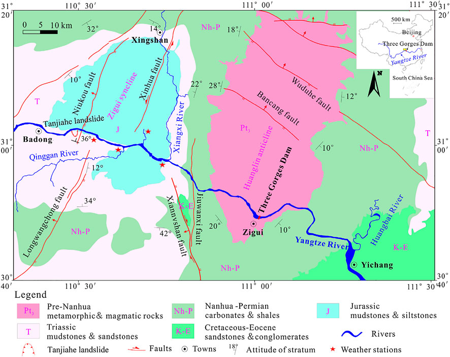
FIGURE 1. Geographic location of Tanjiahe landslide.

FIGURE 2

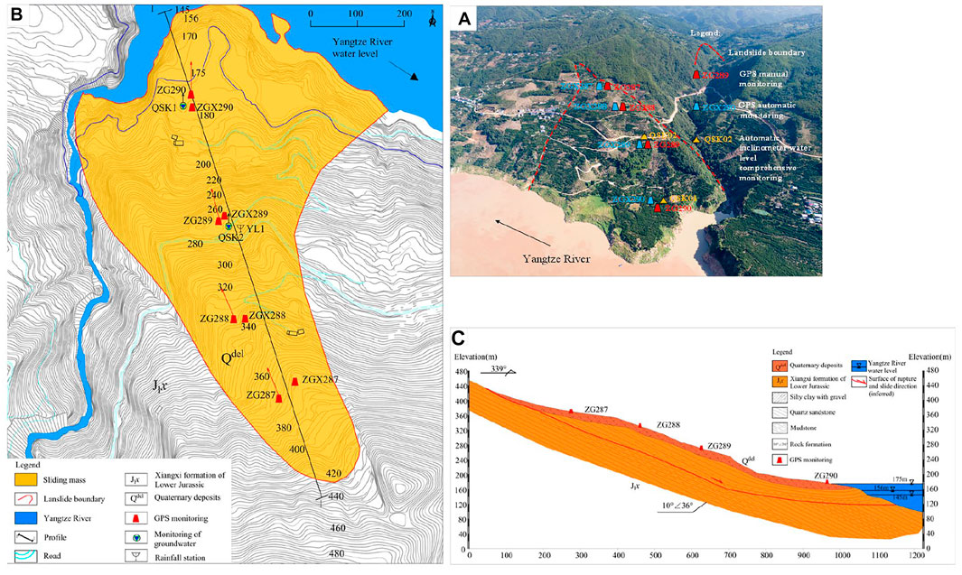
FIGURE 2. Tanjiahe landslide. (A) Panoramic view of the landslide. (B) Planar map of the landslide. (C) Geological profile.

The Three Gorges Reservoir was impounded at 135 m since 2003, 156 m since 2006, and 175 m since 2008. The water level of the reservoir rises and falls between 145 and 175 m every year, and this affects the deformation of the Tanjiahe landslide. Four manual GPS monitoring points, four GPS automatic monitoring points, and two comprehensive monitoring holes for automatic inclination, groundwater level, and water temperature were arranged on the Tanjiahe landslide. The layout of the Tanjiahe landslide monitoring points is shown in Figure 2B, and the professional monitoring profile is shown in Figure 2C.

According to the geological survey and drilling data, the material composition of the Tanjiahe landslide can be divided into: 1) The sliding mass mainly composed of Quaternary colluvial brownish yellow gravelly soil, and the gravels which are composed of sandstone, silty sandstone, and mudstone. The size of the crushed stone varies from 0.1 to 0.3 m. The soil-rock ratio was 5:5–3:7. 2) The sliding zone, which is affected by dynamic action, and mainly composed of heavy silty clay which is yellowish-gray and hard plastic, and breccia composed of sandstone and mudstone caused by the extrusion of the sliding mass. The particle size ranges from 0.1 to 2 mm, and the soil-rock ratio of the sliding zone is 6:4 to 8:2. 3) The sliding bed is composed of two rock layers: the lower Jurassic Xiangxi Group layered quartz sandstone and silt block fracture rock. The sliding bed is composed of layered quartz sandstone and blocky siltstone of Xiangxi formation of Lower Jurassic system. We determine the physical and mechanical properties of Tanjiahe landslide by comparing other similar landslide rocks and soils in the Three Gorges Reservoir area. The basic physical parameters of the slide components are listed in Table 1.

TABLE 1

TABLE 1. Basic physical parameters of slide mass components.

2.2 Surface deformation characteristics

The Tanjiahe landslide is an ancient rock landslide, which was in a state of creep deformation before the June 2003 impoundment of the Three Gorges Reservoir at 135 m. In 2007, the water level of the reservoir reached 156 m for the first time and cracks appeared on the rear edge of the landslide, causing damage to a nearby house (Figure 3A). No obvious signs of deformation were observed before June. From July to September, multiple cracks and small-scale collapses appeared at the middle part and rear edge of the landslide (Figure 3B).

FIGURE 3

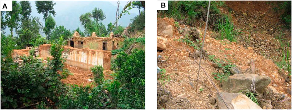
FIGURE 3. The Three Gorges Reservoir was impounded to 156 m for the first time in 2007, resulting in (A) damage to a house caused by cracks in the rear edge of the landslide, (B) small-scale slump in the middle of the landslide.

After the heavy rainfall from August 31 to 2 September 2014, the surface deformation of the landslide was serious, mainly at the northwest boundary of the landslide. The road was severely damaged, and the subgrade sank approximately 1.5 m. The deformation is shown in Figure 4A, where the road pavement is cracked, broken, and upturned, with a displacement distance of 40 cm (Figure 4B). There is a local collapse on the right side of the front edge of the landslide, and a crack of approximately 5 m long near the river edge (Figure 4C).

FIGURE 4

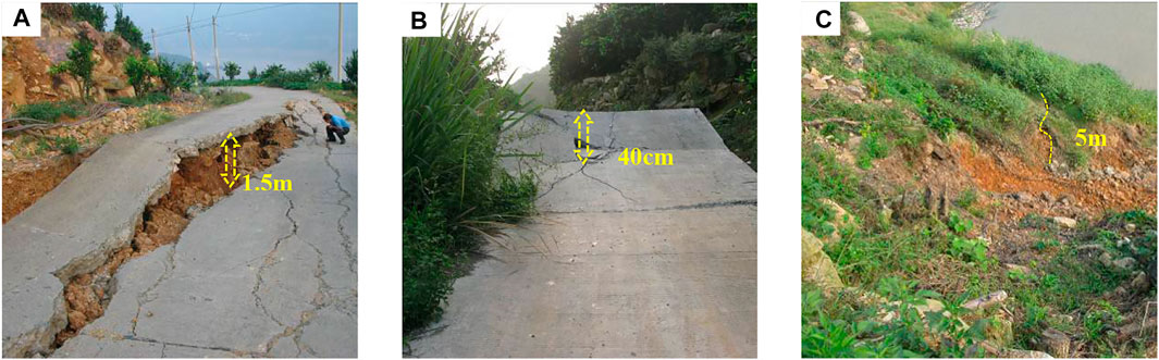
FIGURE 4. Under the influence of heavy rainfall in Zigui (August 31st to 2 September 2014), the landslide surface was seriously deformed. (A) The road was damaged, and the maximum downfall depth was 1.5 m, (B) the road surface was upturned and broken, and (C) the right side of the front edge of the landslide had collapsed and cracked.

In 2016, many cracks appeared on the east and west sides of the middle and rear parts of the landslide, forming a clear landslide boundary (Figure 5A). The overall strike range was 330°–20°, and the collapse could be observed along the crack platform (Figure 5B), with a width of approximately 1–8 mm, and it extended intermittently to the middle highway. At the intersection of the western boundary and the central highway, owing to the continuous deformation of the landslide, the road surface cracks crisscross and are seriously damaged (Figure 5C).

FIGURE 5

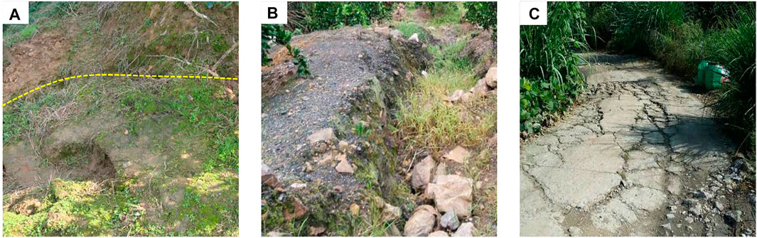
FIGURE 5. There are multiple cracks on both sides of the middle and rear of the landslide (2016). (A) Boundary cracks appear on the east side of the middle and rear of the landslide, (B) on the west side of the rear edge of the landslide, and (C) deformation and damage of the boundary road on the west side of the landslide.

2.3 Groundwater level response

According to Figure 6, the range of the water level rise and fall in the reservoir is at the anti-sliding section of the landslide. The landslide groundwater level data were obtained from two automatic inclination, groundwater level and water temperature comprehensive monitoring holes: QSK1 which is located at 178 m elevation on the slope, and QSK2 which is located at 270 m elevation on the slope. Figure 6 shows the relationship between reservoir water level, rainfall, and groundwater level over the entire monitoring period (June 2016 to August 2019), the groundwater level of monitoring hole QSK1 changed with the reservoir water level. This was conducive to the infiltration of reservoir water, and the change process was essentially synchronized. The groundwater level of monitoring hole QSK2 fluctuates in the range of 236–245 m, and is affected by rainfall. The groundwater level increases with the increase in rainfall (gray area in Figure 6) because the cracks between the fractured rocks are good for seepage and QSK2 is located on a platform (as shown in Figure 2B). The upper part of the sliding mass has low permeability and has the function of storing rainwater. When the rainfall is sufficient, the rainwater collects and the groundwater level rises. When the rainfall decreases, there is not enough rainwater to replenish the groundwater and the groundwater seeps into the lower part of the sliding mass, causing the groundwater level to drop.

FIGURE 6

FIGURE 6. Relationship between groundwater level, rainfall and reservoir water level.

2.4 GPS surface displacement

The Tanjiahe landslide continuously deformed during monitoring. Figure 7 shows the artificial GPS cumulative horizontal displacement of the Tanjiahe landslide is related to fluctuation of the reservoir water level, especially from the initial water storage to the high-water level. For example, when the water level reached 172 m for the first time, the deformation rate increased by approximately 60% compared to the previous year. From November of each year to July of the following year, the cumulative displacement-time curve of each monitoring point shows a distinct upward trend, whereas from August to October each year, the cumulative displacement curve tends to flatten. This phenomenon shows that the displacement rate of the Tanjiahe landslide increased when the water level of the reservoir decreased and decreased when the water level of the reservoir increased.

FIGURE 7

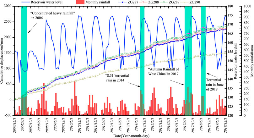
FIGURE 7. Cumulative displacement-time curve of artificial GPS monitoring points of Tanjiahe landslide.

Rainfall had some influence on landslide deformation. After the Three Gorges Reservoir was first filled to 156 m in 2007, owing to concentrated heavy rainfall, the deformation of each monitoring point began to intensify after June (shown in the green area in Figure 7). There were many cracks and collapses at the middle and rear edge of the landslide (Figure 3). During the anomalously heavy “Autumn Rainfall of West China” event in 2017, the rainfall of the Tanjiahe landslide reached 286.8 mm in July and 409 mm from September to October. Strong rainfall led to a sudden increase in the displacement rate (indicated by the pink circle in Figure 7).

The cumulative displacement curve of the landslide shows the displacement of each monitoring point is synchronous, indicating that the landslide is undergoing overall deformation, although some sudden stepwise changes occur at specific times, such as the steps that occurred on 10 June 2015 (63.94 mm) and 22 July 2016 (101.39 mm). The cumulative displacement curve shows an upward trend to varying degrees. The monitoring data indicate that the largest cumulative deformation was at monitoring point ZG289 which is in the middle of the landslide, followed by monitoring points ZG287 and ZG288 which were located on the rear edge of the landslide. The landslide deformation was mainly concentrated in the middle and rear parts, which is consistent with the influence of the terrain. Therefore, it can be inferred that the deformation mode of the landslide was thrust load-caused.

3 Failure process prediction

Once the landslide loses stability under the extreme conditions mentioned above, the sliding mass in the middle and rear will not only destroy nearby houses, roads, bridges, and other infrastructure, but also but also promote the front sliding mass to quickly enter the water, causing swells. This presents a threat to shipping safety and the personal safety of residents in nearby surrounding areas. The next step is to use the MatDEM system to simulate the landslide failure process.

3.1 Theoretical method

The discrete element method is a numerical calculation method based on traditional Newtonian mechanics. First, the resultant external force on the unit is calculated, and then the acceleration is obtained. The entire simulation time is divided into many small time-steps. Therefore, the acceleration and velocity in a certain time step can be regarded as constant values, and the unit displacement can be obtained through the velocity of this time step. The entire motion process of the unit is simulated using iterative operations. $ti$represents a certain moment and $t$ represents the time step size. The equation used is as follows:

$a\left(ti\right)=\frac{F\left(t_i\right)}{m}(1)$

$v\left(t_{\mathrm{i}}\right)=v\left(t_0\right)+a\left(t_{\mathrm{i}}\right)\cdot t(2)$

$x\left(t_{\mathrm{i}}\right)=v\left(t_{\mathrm{i}}\right)\cdot t(3)$

The landslide process involves a variety of energy evolutions. Mechanical energy comprises kinetic, gravitational potential, and elastic potential energy. The units were converted into heat through mutual collisions and friction, and the total energy was composed of mechanical energy and heat. The heat is mainly composed of damping heat, fracture heat and friction heat. In the discrete element numerical simulation, all kinds of heat are calculated and accumulated in each time step through the time step iterative operation.

In the discrete element method, the elastic wave in the model is weakened by damping and the kinetic energy in the discrete element system is dissipated. The damping heat can be calculated by Eq. 4:

$Q_{\mathrm{d}}=-\eta vdx(4)$

$\eta$is the damping coefficient, $v$ is particle velocity. $dx$ is the displacement of particles in the current time step.

The fracture heat is divided into tensile fracture heat ($F_{\mathrm{n}}>0$)and compressive fracture heat ($F_{\mathrm{n}}\le 0$):

$Q_{\mathrm{b}}={\{}_{0.5\left(F_{\mathrm{s}\mathrm{m}\mathrm{a}\mathrm{x}}^2-F{\prime }_{\mathrm{s}\mathrm{m}\mathrm{a}\mathrm{x}}^2\right)/K_{\mathrm{s}},F_{\mathrm{n}}\le 0}^{0.5K_{\mathrm{n}}{X}_{\mathrm{n}}^2+0.5K_{\mathrm{s}}{X}_{\mathrm{s}}^2,F_{\mathrm{n}}>0}(5)$

$K_{\mathrm{n}}$, $K_{\mathrm{S}}$is the normal and tangential stiffness respectively, $X_{\mathrm{n}}$, $X_{\mathrm{S}}$is the normal and tangential relative displacement respectively.

When the tangential force between particles is greater than the maximum internal friction, the particles begin to slide relatively. Friction heat generated during sliding is defined as the product of average sliding friction and sliding distance:

$Q_{\mathrm{f}}=\left|0.5\left(F_{\mathrm{s}1}+F_{\mathrm{s}2}\right)\cdot \mathrm{d}S\right|(6)$

$F_{\mathrm{s}1}$, $F_{\mathrm{s}2}$is the sliding friction at the beginning and end of the current time step respectively, $\mathrm{d}S$is the sliding distance.

The total energy of the unit remains the same when there is no resultant force to perform work. The landslide unit will be subjected to external force in the process of movement, and the total energy will change constantly under the action of external force, so this study only considers the change in kinetic energy. Kinetic energy was calculated as follows:

$E_{\mathrm{k}}=\frac{1}{2}m\cdot v{\left(t_{\mathrm{i}}\right)}^2(7)$

Several theoretical-based numerical analysis software packages have been developed since the establishment of the DEM. At present, MatDEM has been applied to the numerical analysis of geological and geotechnical engineering problems. In this study, the MatDEM system was used to establish a 3D model of the landslide and simulate its failure movement process.

3.2 Establishment of landslide numerical model

The digital elevation of the landslide was obtained and combined with the landslide plan and profile (Figure 2B and Figure 2C), the potential sliding surface was constructed, and the sliding mass was cut out. Because only a weak influence on the deep part of the bedrock during the landslide process, a thin-shell model was established. This greatly reduced the number of particles and thus the calculation time. The longitudinal length of the entire model was 1,445 m, the horizontal length was 915 m, the maximum elevation was 472 m, and the surface elevation of the reservoir was 145 m. The particle radius was distributed around 3.5 m, a total of 440,000 units were created, and the number of sliding mass units was 48,950.

The discrete element method generally simulates materials that match the measured macroscopic mechanical properties by creating particles with specific mechanical properties. In this study, the contact model adopted the linear elastic model, and the microscopic parameters of the particles were mainly obtained from the measured macroscopic parameters through the conversion equation of the macro-and micro-mechanical parameters of close regular packing. The five particle micro-parameters involved in the equation are the normal stiffness of the bond $K\mathrm{n}$, shear stiffness of the bond $K\mathrm{s}$, breaking displacement $X\mathrm{b}$, inter-particle shear resistance $F\mathrm{s}0$, and inter-particle coefficient of friction $\mu \mathrm{p}$, through the five macroscopic mechanical properties of the material: elastic modulus $E$, Poisson’s ratio $v$, compressive strength $C_{\mathrm{u}}$, tensile strength $T_{\mathrm{u}}$, and coefficient of intrinsic friction $\mu \mathrm{i}$ ($\mu \mathrm{i}=\tan \phi$, $\phi$ is the internal friction angle of the material). The conversion equations used for the 3D calculation model are as follows (Liu et al., 2015):

$K_{\mathrm{n}}=\frac{\sqrt{2}Ed}{4\left(1-2v\right)}(8)$

$K_{\mathrm{s}}=\frac{\sqrt{2}\left(1-5v\right)Ed}{4\left(1+v\right)\left(1-2v\right)}(9)$

$X_{\mathrm{b}}=\frac{3K_{\mathrm{n}}+K_{\mathrm{s}}}{6\sqrt{2}\left(K_{\mathrm{n}}+K_{\mathrm{s}}\right)}\cdot T_{\mathrm{u}}\cdot d^2(10)$

$I={\left[{\left(1+{\mu }_{\mathrm{i}}^2\right)}^{1/2}+{\mu }_{\mathrm{i}}\right]}^2(11)$

${\mu }_{\mathrm{p}}=\frac{-2\sqrt{2}+\sqrt{2}I}{2+2I}(12)$

$F{\mathrm{s}}_0=\frac{1-\sqrt{2}{\mu }_{\mathrm{p}}}{6}\cdot C_{\mathrm{u}}\cdot d^2(13)$

Owing to the infiltration of rainfall and reservoir water to reduce the strength of the sliding mass, it is reasonable to use a lower coefficient of intrinsic friction. The micromechanical parameters were obtained using the conversion equation shown in Table 2.

TABLE 2

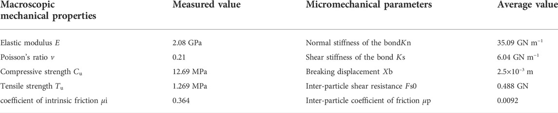
TABLE 2. Macro and micro parameter values of sliding mass material.

After assigning the corresponding parameters of the sliding mass, sliding bed, and water; landslide models with various specific mechanical properties were obtained, as shown in Figure 8A (the underwater terrain of the landslide was excluded). Water was set as a material without friction and strength to simulate the real material, and the force and softening effect of the water on the sliding mass were not considered. The discrete element method calculates the sliding speed of the landslide by considering the influence of terrain factors, which is more suitable for real-world engineering situations. By cutting the sliding mass along the longitudinal direction, the closer it was to the landslide surface unit, the larger the velocity; therefore, this study divided the sliding mass material into nine regions (G1-G9). Three surface monitoring units were set equidistant from the right boundary to the left boundary of the sliding mass in each area, with a total of 27 (M1-M27) monitoring points, to monitor the speed of the front, middle, and rear parts of the sliding mass. To display the monitoring unit clearly, it is enlarged, and the original radius was used in the calculation, as shown in Figure 8B.

FIGURE 8

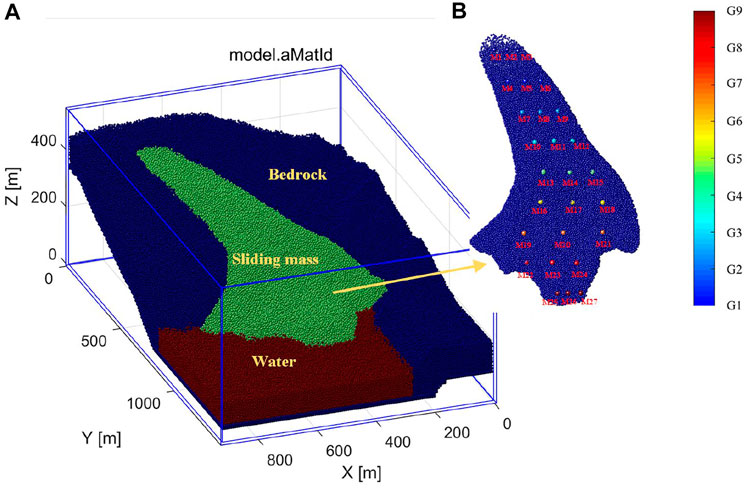
FIGURE 8. Tanjiahe landslide. (A) Numerical model. (B)Layout of landslide monitoring points.

3.3 Numerical simulation results

3.3.1 Displacement distribution changes

By disrupting the connection between the sliding mass and the sliding bed, the landslide is destroyed instantly. However, the iterative operation simulates the process of the landslide continuing to move after failure due to gravity. The model calculation time step was 1×10^–4 s, the total number of iterative calculation steps was 144×10⁴, and the real-world time was set for 144 s. This failure process is shown in Figure 9. The maximum displacement of the sliding mass element did not change significantly after entering the water (Figures 9E–H), the sliding mass at each position slowly piled. Because the kinetic energy of the units has been stable after 96 s, the units no longer produce a large displacement.

FIGURE 9

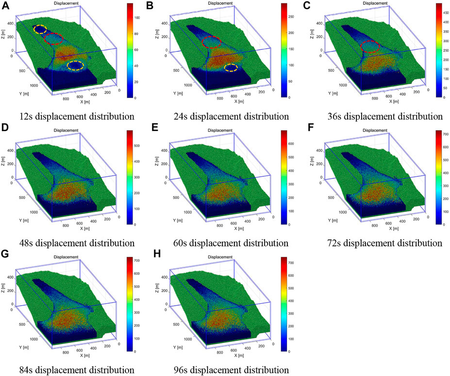
FIGURE 9. Distribution of displacement with time during landslide process (m). (A) 126 s displacement distribution, (B) 246 s displacement distribution, (C) 366 s displacement distribution, (D) 486 s displacement distribution, (E) 606 s displacement distribution, (F) 726 s displacement distribution, (G) 846 s displacement distribution, (H) 966 s displacement distribution.

By comparing the distributions of the units before and after the landslide (Figure 10), movement was detected. The slope of the rear part of the landslide was between 9° and 17°, part of the rear unit remained in place, while a part slid to the middle and covered the upper part of the middle unit. The slope in the middle of the landslide was 20°. The middle unit slid and covered the front. A small number of units collided with the mountain on the left side of the landslide and accumulated in the gully. Because of the steep terrain on the middle right of the landslide (as shown in Figure 2A), the units with the largest sliding distance in the middle and rear were piled up on the front right platform of the landslide, with a maximum displacement of 775 m. The slope at the front of the landslide was only 8° and the maximum sliding distance of the front unit was 598 m, as shown in Figure 10B. This showed that the slope was an important factor that affects the sliding distance.

FIGURE 10

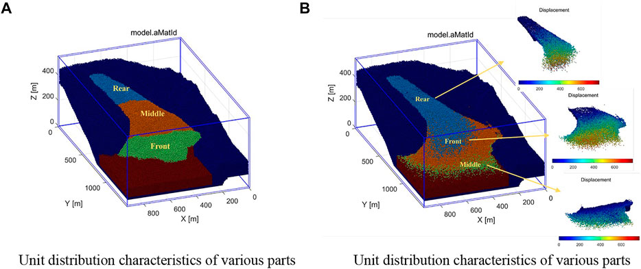
FIGURE 10. Unit distribution characteristics of various parts before and after landslide. (A) Unit distribution characteristics of various parts before landslide, (B) Unit distribution characteristics of various parts after landslide.

3.3.2 Movement speed changes

The elastic strain energy of the landslide was released at the instant of failure, and the average velocity of the all sliding element showed a rapid increase at first, reaching a peak velocity of 4.76 m/s at 25 s. During the sliding process, the energy dissipated by friction and collision caused the unit speed to decrease rapidly after reaching the peak value. When the average speed reached 1.77 m/s, the average speed decreased slowly and did not approach 0 m/s until 144 s. The speed change during the landslide process can be divided into three stages: rapid rise, rapid decline, and slow decline (Figure 11).

FIGURE 11

FIGURE 11. Average velocity of sliding mass units.

The dynamic change in the monitoring unit’s speed during the sliding process was recorded as a graph of the change in speed over time at point. Figure 12 show that the velocity curve fluctuated due to the constant collision between the units during the sliding process. This sudden change can be divided into two types: rear block decelerated by collision and front block accelerated by collision (Ge et al., 2021). That is, the speed of the front-sliding mass is suddenly increased by the rear collision, and the speed of the rear-sliding mass is suddenly reduced by the front blocking (Figure 12B). Every three monitoring points at the same longitudinal position had similar velocity variation characteristics, but under the influence of special terrains, such as steep cliffs and gullies, the velocity of a unit may increase abnormally and become difficult to stabilize (shown in the orange area in Figure 12A,I).

FIGURE 12

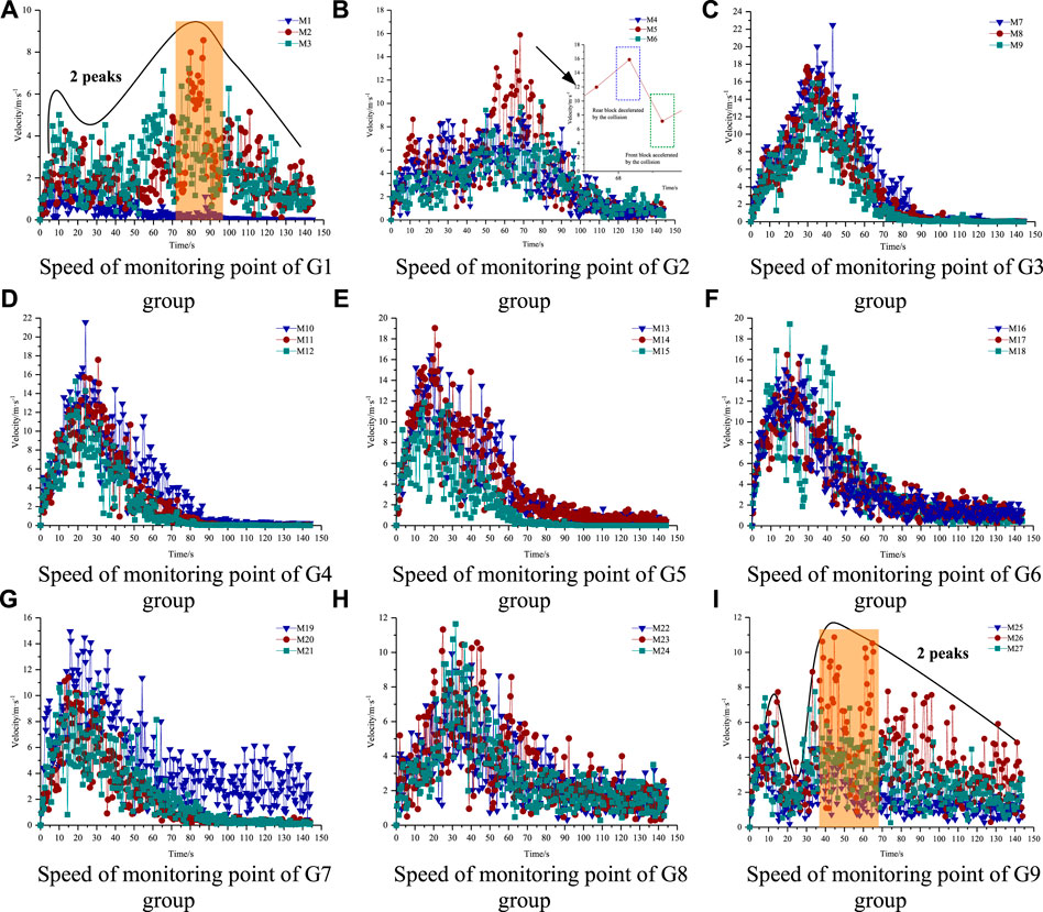
FIGURE 12. Speed of sliding mass monitoring unit. (A) Speed of monitoring point of G1, (B) Speed of monitoring point of G2, (C) Speed of monitoring point of G3, (D) Speed of monitoring point of G4, (E) Speed of monitoring point of G5, (F) Speed of monitoring point of G6, (G) Speed of monitoring point of G7, (H) Speed of monitoring point of G8, (I) Speed of monitoring point of G9.

3.3.3 Energy evolution

The landslide process was accompanied by energy conversion. All energy was initialized before breaking the bond between the sliding mass and the sliding bed to ensure that the energy change was not affected by the process of establishing the landslide model before failure. Figure 13 shows that due to gravity, the Tanjiahe landslide converted 8.0×10¹² J gravitational potential energy into other forms of energy. Only a small portion was converted into kinetic energy, and the kinetic energy peak appeared at 28 s. The conversion rate of gravitational potential energy to kinetic energy was only 20%. Until the model energy stabilized, 93% of the gravitational potential energy was predominantly dissipated in the form of frictional heat with limited conversion into any other heat energy types. Numerous collisions and friction occurred between the landslide units during the traveling process, and the dissipated heat increased continuously. During the landslide process, despite the large drop between the front and rear edges of the landslide and the initial increase in kinetic energy, the longitudinal length of the landslide was also large and once the sliding mass started to move in the long term, the kinetic energy decreased rapidly because of collisions and friction.

FIGURE 13

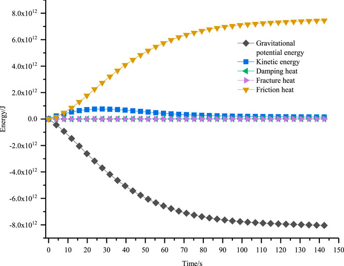
FIGURE 13. Energy conversion during landslide process.

4 Discussion

4.1 Influencing factors and the deformation mechanism

The deformation of the Tanjiahe landslide between 1 June 2016, and 31 December 2019, was divided into three hydrological years to account for the rise and fall of the water level of reservoirs as shown in Figure 14: Stage I is 2016/11/1–2017/10/31, Stage II is 2017/11/1–2018/10/31, and Stage III 2018/11/1–2019/10/31. The cumulative displacement over the three stages showed that when a high-water level was falling, the displacement rate of each monitoring point was significantly greater than when a low-water level was rising (the red arrow is steeper than the black arrow in Figure 14). During the a-d period of Stage I, the reservoir water level was running at 175 m and dropped to approximately 145 m. The displacement rates of the automatic monitoring points ZGX287, ZGX288, ZGX289, and ZGX290 during this period were 0.38, 0.36, 0.39, and 0.22 mm/d, respectively. During the d to e period of late Stage I to Stage II, the reservoir water level rose from approximately 145–175 m. The displacement rates of the fully automatic monitoring points ZGX287, ZGX288, ZGX289, and ZGX290 during this period were 0.25, 0.20, 0.25, and 0.13 mm/d, respectively. The data showed that the displacement rate during the a-d phase (during the falling reservoir water level) was 1.8 times greater than that of the d-e phase (during the rising reservoir water level). The results showed that landslide deformation was affected by the high-level operation of the reservoir and the decrease in the reservoir water level.

FIGURE 14

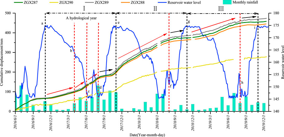
FIGURE 14. Cumulative displacement-time curve of Tanjiahe landslide automatic GPS monitoring point.

During the period from b-c of the Stage I, the reservoir water level dropped from 165 m to about 145 m, and the reservoir water drop rate was -0.27 m/day. The displacement rates of the automatic monitoring points ZGX287, ZGX288, ZGX289, and ZGX290 during this period were 0.52, 0.50, 0.50, and 0.29 mm/d, respectively. During the b-d period of the Stage I, the reservoir water level dropped from 165 m to about 145 m, and the drawdown rate was −0.14 m/day, the displacement rates of the automatic monitoring points ZGX287, ZGX288, ZGX289,r water in the b-c phase was twice that of the b-d phase, but the corresponding displacement rate was not significantly different, which indicates that the landslide deformation was hardly affected by the drawdown rate of the reservoir water level.

During the period of d-e, the rainfall suddenly increased, and the reservoir water level reached the highest water level (175 m) on 2017/10/31. The deformation of the Tanjiahe landslide started at this time and the displacement rate reached 0.9 mm/d. After heavy rainfall, the displacement rate of the landslide was 2–3 times higher than previous rates during the period a-d in Stage I and period g-h in Stage III, as shown in Figure 14. This phenomenon demonstrated that an increase in rainfall had a significant effect on landslide deformation.

From the profile of the Tanjiahe landslide (Figure 2C), the shape of the sliding surface was steep at the top and gentle at bottom. The dip angle of the middle and rear parts of the sliding surface was 20°, and the length, which is the sliding section of the landslide was approximately 700 m. The front dip angle was 8°, which is the anti-sliding section of the landslide and the affected by the reservoir water fluctuation (Figure 2C). The thickness of the sliding mass was 60–90 m. In addition, the front of the landslide was approximately 400 m long and 600 m wide (Figure 2B), making it difficult for reservoir water to infiltrate the slope. By comparing the physical and mechanical properties of other similar landslide rocks and soils in the Three Gorges Reservoir area, the permeability of Tanjiahe landslide mass is obtained. The deep part of the sliding mass was fractured quartz sandstone (145–156 m) with high permeability and a permeability coefficient of 3.456 m/d, its surface layer was a loose accumulation of material (156–175 m), with low permeability and a permeability coefficient of 0.432 m/d, and a thickness of 19 m as shown in Figure 2C. Due to the difference in permeability between the deep and surface layers, when the reservoir water level ranged from 145 to 175 m, the floating force on the sliding mass was not large, and a seepage force was generated and directed to the inside of the slope, which increased the stability of the slope mass through back pressure. When the reservoir water level was at the high-water level (175 m), the groundwater level in the slope mass rose to this level. At that point, the floating force on the sliding mass was the largest and the displacement rate increased. When the reservoir water level ranged from 175 to 156 m, it was difficult for the reservoir water to seep out of the surface of the sliding mass. The combined floating force and seepage force work together, resulted in an increase in the displacement rate. When the reservoir water level was 156–145 m, the groundwater level in the slope lagged behind the reservoir water level, resulting in a seepage force, which also increased the displacement rate.

According to the above analysis of the surface deformation characteristics and displacement monitoring data of the Tanjiahe landslide, the inconsistent permeability of various parts of the landslide, the reservoir running with a high-water level and drawdown of the reservoir water level were the key factors affecting the deformation of the Tanjiahe landslide, especially the first water storage to the high-water level. Increased rainfall caused local collapse of the shallow soil mass, and the rainwater infiltration reduced the shear strength of the sliding zone, which promoted the deformation of the Tanjiahe landslide. The gentle terrain in the front part, which is the anti-sliding section; the middle and rear part creep along the layer along the weak slip belt, which is the sliding section. Under conditions of high-water level operation and water level drawdown, the anti-sliding section of the sliding mass was subject to superposition of the floating force and seepage force. Therefore, the stability of the anti-sliding section was reduced, the sliding section was displaced by the driving force, and the deformation mode of the landslide was typical thrust load-caused.

After heavy rainfall, the Tanjiahe landslide could easily fail under extreme working conditions of high-water level operation or water level drawdown. Because most of the Tanjiahe landslide is composed of fragmented rock blocks, upon failing it will likely form a high-speed debris flow. This will not only wash away houses, roads and vegetation, but also form a surge when entering the reservoir and expand the range of the disaster further and cause additional losses.

4.2 Motion characteristics analysis and potential risk prediction

According to the displacement distribution in the early stage of the landslide movement (12–36 s), unit displacement mainly distributed in the front and rear of the landslide was 0 m (indicated by the yellow circle in Figure 9A). At this time (12 s), the maximum displacement of the middle unit reached 100 m and the maximum displacement of the rear unit reached 60 m. Afterwards, some of the units at the rear of the sliding mass move continuously with the middle unit (the red circle moves in Figures 9A–C). The number of units at the front without displacement decreases with time (the yellow circle in Figure 9B is smaller than that in Figure 9A). Therefore, in the early stage of the landslide, large-scale sliding occurred simultaneously in the middle and rear of the landslide, moved to the front of the landslide, and finally pushed the front-sliding mass into the water body, which belongs to the failure mode of the upper sliding mass pushing the lower sliding mass. This is consistent with the deformation mode of the landslide described in Section 2.

The maximum speed reached by the sliding mass unit of the Tanjiahe landslide was 23 m/s (Figure 12). According to the classification of landslides according to sliding speed by IAEG (Zhang et al., 2016), Tanjiahe landslide is close to that of ultra-high-speed landslides (25–30 m/s). These are easily converted into extremely fast debris flows. The change in the velocity at the monitoring points of each part (Figure 12), showed that the change trend was consistent with that of the average velocity of the sliding mass unit, and had also experienced the rapid rise, rapid decline, and slow decline stages (Figure 11). The speed change of the rear monitoring units was analyzed. The G1 group unit showed a peak value of 5 m/s at 10 s and then decreased, and then a second peak value of 9 m/s at 84 s (Figure 12A). The speed of the G2 group unit peaked at 16 m/s at 68 s (Figure 12B) and the speed of the G3 group unit peaked at 23 m/s at 36 s (Figure 12C). Analyzing the speed change of the middle monitoring unit, the units G4-G6 reached the speed peak at 20–24 s, and the peak value was 19–21 m/s, then declined first rapidly, then slowly and after 96 s, the velocity fluctuated close to zero (Figures 12D–F). The speed change of the rear front units was analyzed. The speed of the G7 group unit peaked at 22 m/s at 17 s (Figure 12G). The speed of the G8 group unit peaked at 12 m/s at 33 s (Figure 12H). The G9 group unit showed a peak value of 8 m/s at 10 s and then decreased, and then a second peak value of 11 m/s at 45 s (Figure 12I). The G8 and G9 groups did not experience a rapid decline, and the velocity fluctuated continuously. Compared to the other units, when G8 and G9 collided with water which has a low elastic modulus, the velocity declined slowly, and constantly fluctuated in the low value range. During the landslide process, the speeds of the G1 at the front edge and G9 at rear edge showed a bimodal characteristic (shown by the trend of the black curves in Figure 12A,I). This is because the G1 group unit accelerated after being pulled by the front unit, and decelerated after colliding with the front unit, whereas the front unit kept moving. This caused the rear unit to lose support and start to accelerate again. The G9 group unit collided with the rear unit, and then decelerated after colliding with the water. At this point, they collided with the rear unit and started to accelerate again. This showed that the monitoring units in each section show different motion processes, and distinct differences in the velocity peak time point and velocity peak value of the unit. The time points of the rear and front monitoring units have smaller slope angles, reached the peak speed later and had smaller peak values than those of the middle monitoring units. The analysis showed that the larger the angle of the slope, the higher the acceleration in the direction parallel to the slope surface, and the faster the unit accelerated to the peak velocity. The value of the peak velocity was also positively correlated with the slope angle, and the displacement generated at the same time was greater.

Because the total energy changed owing to the work done by the external force during the movement of the monitoring unit, and the value of the gravitational potential energy relative to the kinetic energy was too large, only the kinetic energy change characteristics were analyzed. The kinetic energy of the rear monitoring unit was analyzed, and the kinetic energy evolution characteristics of the G3, G2, and G1 units were consistent with the speed variation characteristics (Figure 15A). Analyzing the kinetic energy of the monitoring unit in the middle showed little difference in the magnitude and change trend of the kinetic energy of the G4-G6 units (Figure 15B). Analyzing the kinetic energy of the front monitoring unit, the G7 unit collided with G8 after the movement, resulting in an increase in the kinetic energy of G8; the kinetic energy of G9 increased again after being hit by G8 (Figure 15C). This was attributed to the energy transfer phenomenon in the front unit during the landslide process, and the energy that was transferred between the units through collision.

FIGURE 15

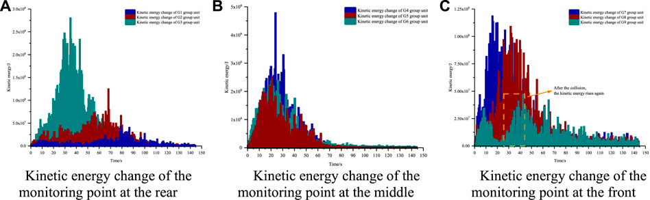
FIGURE 15. Kinetic energy change of sliding mass monitoring unit at each parts. (A) Kinetic energy change of the monitoring point at the rear, (B) Kinetic energy change of the monitoring point at the middle, (C) Kinetic energy change of the monitoring point at the front.

According to the simulation results of the final stacking range of the landslide, the rock and soil units in the middle and rear of the landslide produced a large displacement away from the original position, and the middle unit slipped above the front unit. As shown in Figure 2A, there are houses in front of the landslide, and once the landslide reactivates, the front house will be washed away. In addition to causing damage to vegetation and buildings, reservoir rock landslides may also form surges, which have a wide range of impacts and great destructive power. Yin et al. (2012) conducted a model test of landslide surges in the Three Gorges Reservoir and proposed an equation for calculating the height of first wave of a landslide in the Three Gorges Reservoir. The equation considers important parameters such as the scale, shape, and water entry angle of the landslide, as follows:

$\frac{H\max }{h}=1.17\frac{v}{\sqrt{gh}}\left({\sin }^2\alpha +0.6{\cos }^2\alpha \right){\left(\frac{lt}{bh}\right)}^{0.15}{\left(\frac{w}{b}\right)}^{0.45}(14)$

where $v$ is the water entry speed of the sliding mass and $\alpha$ is the inclination angle of the sliding belt. $l$ , $w$ , and $t$ are the average longitudinal length, average width, and average thickness of the landslide entering the water, respectively; $h$ is the maximum static water depth at which the landslide enters the water, and $b$ is the width of the channel at the water inlet section.

The calculation equation of cross-section propagation wave height is as follows:

$\frac{H\mathrm{p}}{h}=1.47\frac{H\max }{h}{\left(\frac{x}{h}\right)}^{-0.5}\left(\frac{x}{h}>2.13\right)(15)$

where $x$ is the propagation distance from the bank to the opposite bank.

The equation for calculating the propagation wave height along the route is as follows:

$\frac{H\mathrm{r}}{h}=\frac{H\max }{h}{e}^{-0.4{\left(\frac{x}{h}\right)}^{0.35}}(16)$

In this equation, $x$ is the distance from somewhere along the route to the landslide. The following figure (Figure 16) is a schematic diagram explaining the propagating waves along the cross section and along the route.

FIGURE 16

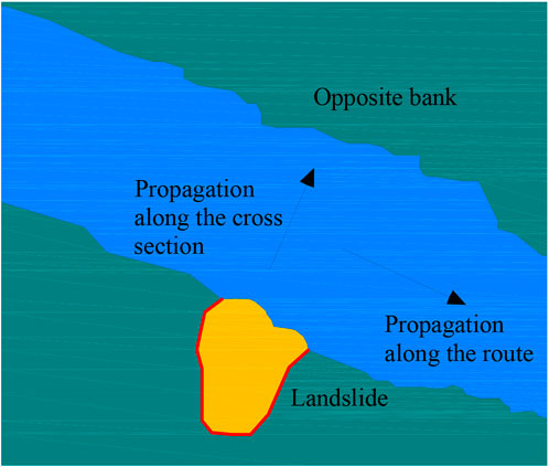
FIGURE 16. Schematic diagram of wave propagation.

The numerical simulation results of the landslide (Figure 10B) show that some units at the front of the landslide slide into the water and push the water, indicating that the surge formed by the water entry of the landslide unit needs to be considered. In this study, the maximum first wave height, cross-sectional propagation wave height, and propagation wave height along the route of the landslide under 145 m reservoir water level are calculated.

According to the numerical simulation results, it can be seen that the number of units entering the water area did not increase significantly after 72 s (Figure 9F) Therefore, we used the average velocity 4.435 m/s of the sliding mass units entering water before 72 s as the water entry speed $v$ through Figure 17. The inclination angle $\alpha$ of the sliding surface was 8°, the average length $l$ of the water-entry sliding mass was 251 m, the average width $w$ of the water-entry sliding mass was 386 m, the average thickness $t$ of the water-entry sliding mass was 35 m, the maximum static water depth $h$ at the water entry point of the landslide was 50 m, and the width $b$ of the channel at the water entry section of the landslide was 400 m. After calculation using Eq. 14, the maximum first wave height $H\max$ is 6.13 m.

FIGURE 17

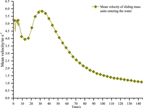
FIGURE 17. Mean velocity of sliding mass units entering water with time during landslide process.

Substituting the relevant parameters into Eq. 15, the wave height that propagated to the opposite bank was 3.67 m. Substituting the relevant parameters into Eq. 16, the relationship between the propagating wave height along the route and the distance from somewhere along the route to the landslide point is as follows:

$H\mathrm{r}=6.13e^{-0.4{\left(\frac{x}{50}\right)}^{0.35}}(17)$

The relationship between the wave height propagating along the route and the distance from somewhere along the route to the landslide point is shown in Figure 18. It shows exponential attenuation characteristics. When the distance from the landslide point was 30 km, the propagating wave height was only 0.14 m, and the surge beyond 30 km was almost harmless. Therefore, the range of influence of the propagating waves along the path was within 30 km.

FIGURE 18

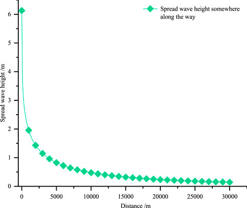
FIGURE 18. Propagation wave height along the route.

5 Conclusion

Using the Tanjiahe landslide, a typical rock landslide in the Three Gorges Reservoir Area, as a case study, the landslide surface deformation, GPS displacement, and groundwater level data under the action of reservoir water-level fluctuation were analyzed and discussed. The influencing factors and deformation characteristics of the reservoir rock landslide were determined. Landslide failure may result in high-speed debris flow, endangering lives, and shipping safety in the reservoir area. To predict the exact disaster-affected area of the Tanjiahe landslide, a numerical model of the landslide was established using the MatDEM system. The connection between the sliding mass and the sliding bed was disrupted, and the movement process of the landslide under the action of gravity was simulated. The main conclusions are as follows:

1) The internal factors influencing Tanjiahe landslide are the landslide morphology and material composition of the landslide. The middle and rear parts of the landslide had steeper slopes, which were the sliding sections of the landslide. The front edge is gentle, which is the anti-sliding section of the landslide, and the range of the reservoir water variation is the anti-sliding section of the landslide. Because the surface sliding mass is a loose accumulation layer (156–175 m) with low permeability and the deep is fractured quartz sandstone (145–156 m) with high permeability, the change in groundwater level in the slope mass has a hysteresis in the range of 156–175 m. The floating force caused by the high-water level operation of the reservoir and the seepage force caused by the drop, as well as the combined action of the two, are the key external factors leading to the deformation of the Tanjiahe landslide. Rainfall had a positive effect on landslide deformation. Under the combined action of flotation and seepage forces, the stability of the anti-sliding section of the sliding mass decreases, and the displacement of the sliding section is significantly larger under the action of the driving force, which belongs to a typical thrust load-caused deformation mode. Under extreme conditions of high-level reservoir operation or a decline in the reservoir water level and the combined action of heavy rainfall, the Tanjiahe rock landslide is prone to instability, forming a high-speed debris flow, posing a threat to the safety of the reservoir area.

2) The numerical simulation results show that when the landslide is destroyed instantaneously, large-scale sliding occurs in the middle and rear of the landslide simultaneously After the middle and rear-sliding masses move to the front of the landslide, the sliding mass at the front is pushed into the water, which belongs to the destruction mode, where the upper sliding mass pushes the lower sliding mass. This is consistent with the deformation mode of the landslide described in Section 2. There are clear differences in the peak time and peak value of the velocity of the monitoring unit in each part, which are closely related to the slope terrain. The analysis shows that when the shear strength parameters of the sliding surface are the same, the larger the slope angle, the higher is the acceleration parallel to the slope surface direction, and the faster the units accelerate to the peak velocity. The peak velocity value is positively correlated with the slope angle and the larger the displacement in the same time.

3) Many collisions and friction occurred between the landslide units, and the dissipated heat continued to increase. Most of the gravitational potential energy is dissipated in the form of frictional heat, and only a small portion is converted into kinetic energy. During the landslide process, there was an obvious energy transfer phenomenon between the units, and energy was transferred between the units through collisions.

4) The stacking range of the numerical simulation shows that the houses on the front of the landslide are vulnerable to being washed away by the rock and soil mass, and the front-sliding mass entering the water causes a surge. The height of the largest first wave generated is 6.13 m, and the wave height that propagates to the opposite bank is 3.67 m, and the influence range of the waves propagating along the route in reservoir area is within 30 km.

Data availability statement

The original contributions presented in the study are included in the article/Supplementary Material, further inquiries can be directed to the corresponding author.

Author contributions

All authors listed have made a substantial, direct, and intellectual contribution to the work and approved it for publication.

Funding

This work was Funded by National Key Research and Development Project (2021YFC3001901), National Natural Science Foundation of China (U21A2031), China Postdoctoral Science Foundation (2021M701969) and Open Fund of Badong National Observation and Research Station of Geohazards (No. BNORSG-202207).

Conflict of interest

The authors declare that the research was conducted in the absence of any commercial or financial relationships that could be construed as a potential conflict of interest.

Publisher’s note

All claims expressed in this article are solely those of the authors and do not necessarily represent those of their affiliated organizations, or those of the publisher, the editors and the reviewers. Any product that may be evaluated in this article, or claim that may be made by its manufacturer, is not guaranteed or endorsed by the publisher.

References

Chang, W. B., Wang, P., Wang, H. J., Chai, S., Yu, Y., and Xu, S. (2021). Simulation of the Q2 loess slope with seepage fissure failure and seismic response via discrete element method. Bull. Eng. Geol. Environ. 80, 3495–3511. doi:10.1007/s10064-021-02139-z

CrossRef Full Text | Google Scholar

Chen, H. R., Qin, S. Q., Xue, L., and Xu, C. (2021). Why the Xintan landslide was not triggered by the heaviest historical rainfall: Mechanism and review. Eng. Geol. 294, 106379. doi:10.1016/j.enggeo.2021.106379

CrossRef Full Text | Google Scholar

Comegna, L., Picarelli, L., and Urciuoli, G. (2007). The mechanics of mudslides as a cyclic undrained-drained process. Landslides 4 (03), 217–232. doi:10.1007/s10346-007-0083-2

CrossRef Full Text | Google Scholar

Ge, Y. F., Tang, H. M., and Li, C. D. (2021). Mechanical energy evolution in the propagation of rock avalanches using field survey and numerical simulation. Landslides 8 (11), 3559–3576. doi:10.1007/s10346-021-01750-1

CrossRef Full Text | Google Scholar

He, C. C., Hua, X. L., Tannant, D. D., Tan, F., Zhang, Y., and Zhang, H. (2018). Response of a landslide to reservoir impoundment in model tests. Eng. Geol. 247, 84–93. doi:10.1016/j.enggeo.2018.10.021

CrossRef Full Text | Google Scholar

Hu, X. D., Zhang, L., Hu, K. H., et al. (2022). Modelling the evolution of propagation and runout from a gravel–silty clay landslide to a debris flow in Shaziba, southwestern Hubei Province, China Landslides.

Google Scholar

Huang, X. H., Guo, F., Deng, M. L., Yi, W., and Huang, H. (2020). Understanding the deformation mechanism and threshold reservoir level of the floating weight-reducing landslide in the Three Gorges Reservoir Area, China. Landslides 17 (12), 2879–2894. doi:10.1007/s10346-020-01435-1

CrossRef Full Text | Google Scholar

Ibanez, J. P., and Hatzor, Y. H. (2018). Rapid sliding and friction degradation: Lessons from the catastrophic Vajont landslide. Eng. Geol. 244, 96–106. doi:10.1016/j.enggeo.2018.07.029

CrossRef Full Text | Google Scholar

Liu, C., Pollard, D. D., Gu, K., and Shi, B. (2015). Mechanism of formation of wiggly compaction bands in porous sandstone: 2. Numerical simulation using discrete element method. J. Geophys. Res. Solid Earth 120 (12), 8153–8168. doi:10.1002/2015jb012374

CrossRef Full Text | Google Scholar

Liu, C., Shi, B., Gu, K., et al. (2014). Development and application of large-scale discrete element simulation system for rock and soil. J. Eng. Geol. 22, 551. doi:10.13544/j.cnki.jeg.2014.s1.092

CrossRef Full Text | Google Scholar

Liu, Z. Y., Su, L. J., Zhang, C. L., Iqbal, J., Hu, B., and Dong, Z. (2020). Investigation of the dynamic process of the Xinmo landslide using the discrete element method. Comput. Geotechnics 123, 103561. doi:10.1016/j.compgeo.2020.103561

CrossRef Full Text | Google Scholar

Luo, S. L., and Huang, D. (2020). Deformation characteristics and reactivation mechanisms of the Outang ancient landslide in the Three Gorges Reservoir, China. Bull. Eng. Geol. Environ. 79 (08), 3943–3958. doi:10.1007/s10064-020-01838-3

CrossRef Full Text | Google Scholar

Ouyang, C. J., Zhao, W., Xu, Q., Peng, D., Li, W., Wang, D., et al. (2018). Failure mechanisms and characteristics of the 2016 catastrophic rockslide at Su village, Lishui, China. Landslides 15 (07), 1391–1400. doi:10.1007/s10346-018-0985-1

CrossRef Full Text | Google Scholar

Song, K., Wang, F. W., Yi, Q. L., and Lu, S. (2018). Landslide deformation behavior influenced by water level fluctuations of the Three Gorges Reservoir (China). Eng. Geol. 247, 58–68. doi:10.1016/j.enggeo.2018.10.020

CrossRef Full Text | Google Scholar

Sun, G. H., Yang, Y. T., Jiang, W., and Zheng, H. (2017). Effects of an increase in reservoir drawdown rate on bank slope stability: A case study at the three Gorges reservoir, China. Eng. Geol. 221, 61–69. doi:10.1016/j.enggeo.2017.02.018

CrossRef Full Text | Google Scholar

Wang, S. M., Pan, Y. C., Wang, L., Guo, F., Chen, Y., and Sun, W. (2021). Deformation characteristics, mechanisms, and influencing factors of hydrodynamic pressure landslides in the three Gorges reservoir: A case study and model test study. Bull. Eng. Geol. Environ. 80 (04), 3513–3533. doi:10.1007/s10064-021-02120-w

CrossRef Full Text | Google Scholar

Wang, W. P., Yin, Y. P., Wei, Y. J., Zhu, S., Li, J., Meng, H., et al. (2021). Investigation and characteristic analysis of a high-position rockslide avalanche in Fangshan District, Beijing, China. Bull. Eng. Geol. Environ. 80 (03), 2069–2084. doi:10.1007/s10064-020-02098-x

CrossRef Full Text | Google Scholar

Xia, M., Ren, G. M., Zhu, S. S., and Ma, X. L. (2015). Relationship between landslide stability and reservoir water level variation. Bull. Eng. Geol. Environ. 74 (03), 909–917. doi:10.1007/s10064-014-0654-0

CrossRef Full Text | Google Scholar

Xu, Q., Fan, X. M., Huang, R. Q., Yin, Y., Hou, S., Dong, X., et al. (2010). A catastrophic rockslide-debris flow in wulong, chongqing, China in 2009: Background, characterization, and causes. Landslides 7 (01), 75–87. doi:10.1007/s10346-009-0179-y

CrossRef Full Text | Google Scholar

Xu, Q., Li, Y. R., Zhang, S., and Dong, X. (2016). Classification of large-scale landslides induced by the 2008 Wenchuan earthquake, China. Environ. Earth Sci. 75 (01), 22. doi:10.1007/s12665-015-4773-0

CrossRef Full Text | Google Scholar

Yao, W. M., Li, C. D., Zuo, Q. J., Zhan, H., and Criss, R. E. (2019). Spatiotemporal deformation characteristics and triggering factors of Baijiabao landslide in Three Gorges Reservoir region, China. Geomorphology 343, 34–47. doi:10.1016/j.geomorph.2019.06.024

CrossRef Full Text | Google Scholar

Yi, X. Y., Feng, W. K., Wu, M. T., et al. (2022). The initial impoundment of the baihetan reservoir region (China) exacerbated the deformation of the wangjiashan landslide: Characteristics and mechanism Landslides. https://doi. org/10.1007/s10346-022-01897-5.

Google Scholar

Yin, K. L., Liu, Y. L., Wang, Y., et al. (2012). Physical model experiments of landslide-induced surge in three Gorges reservoir. Earth Sci. 37 (05), 1067. doi:10.3799/dqkx.2012.113

CrossRef Full Text | Google Scholar

Yin, Y. P., Huang, B. L., Chen, X. T., Liu, G., and Wang, S. (2015). Numerical analysis on wave generated by the qianjiangping landslide in three Gorges reservoir, China. Landslides 12 (02), 355–364. doi:10.1007/s10346-015-0564-7

CrossRef Full Text | Google Scholar

Yin, Y. P., Wang, F. W., and Sun, P. (2009). Landslide hazards triggered by the 2008 Wenchuan earthquake, Sichuan, China. Landslides 6, 139–152. doi:10.1007/s10346-009-0148-5

CrossRef Full Text | Google Scholar

Yu, H. B., Li, C. D., Zhou, J. Q., Chen, W., Long, J., Wang, X., et al. (2020). Recent rainfall- and excavation-induced bedding rockslide occurring on 22 October 2018along the Jian-En expressway, Hubei, China. Landslides 17 (11), 2619–2629. doi:10.1007/s10346-020-01468-6

CrossRef Full Text | Google Scholar

Zhang, Z. Y., Wang, S. T., Wang, L. S., et al. (2016). Principles of engineering geological analysis. Beijing: Geological Publishing House. (in Chinese).

Google Scholar

Zhou, J. W., Cui, P. I., and Hao, M. H. (2016). Comprehensive analyses of the initiation and entrainment processes of the 2000 Yigong catastrophic landslide in Tibet, China. Landslides 13 (01), 39–54. doi:10.1007/s10346-014-0553-2

CrossRef Full Text | Google Scholar

Zhou, J. W., Xu, F. G., Yang, X. G., Yang, Y. C., and Lu, P. y. (2016). Comprehensive analyses of the initiation and landslide-generated wave processes of the 24 June 2015 Hongyanzi landslide at the Three Gorges Reservoir, China. Landslides 13 (03), 589–601. doi:10.1007/s10346-016-0704-8

CrossRef Full Text | Google Scholar