Three-dimensional displacement field of the 2010 Mw 8.8 Maule earthquake from GPS and InSAR data with the improved ESISTEM-VCE method

The 2010 Mw 8.8 Maule earthquake occurred offshore central Chile and ruptured ∼500 km along the megathrust fault resulting from the oceanic Nazca plate subducting beneath the continental South American plate. The Maule earthquake produced remnant crustal displacements captured by a vast set of geodetic observations. However, given the nature of the observational techniques, it is challenging to extract its accurate three-dimensional coseismic deformation field with high spatial resolution. In this study, we modified the extended simultaneous and integrated strain tensor estimation from geodetic and satellite deformation measurements (ESISTEM) method with variance component estimation algorithm (ESISTEM-VCE) to retrieve the three-dimensional surface displacement field of this event by integrating the interferometric synthetic aperture radar (InSAR) and global positioning system (GPS) measurements. The ESISTEM-VCE method accounts for the spatial correlation of surface displacement among the adjacent points and determine the accurate weight ratios for different data sets, but also uses the uncertainties of GPS data and considers the different spatial scales from the different datasets. In the simulation experiments, the RMSEs of the ESISTEM-VCE method are smaller than those of the ESISTEM and ESISTEM-VCE (same d0) methods, and the improvements of 97.1%, 3.9%, and 84% are achieved in the east-west, north-south, and vertical components, respectively. Then, we apply the proposed methodology to the 2010 Mw 8.8 Maule earthquake, to obtain a three-dimensional displacement field that could provide fine deformation information. In the east-west component, the significant deformation is in the north of the epicenter, closed to the Constitución, with a maximum westward displacement of 495.5 cm. The displacement in the north-south component is relatively small compared to that in the east-west component. The maximum uplift reaches 211.8 cm, located at the southwest of the Concepción. Finally, the derived vertical displacements are also compared with field investigations, indicating that the ESISTEM-VCE method can obtain more accurate weight of different datasets and perform better than the ESISTEM method. The results highlight that the earthquake ruptured along the NE-SW direction, with a dominant thrust and a relatively small component of right-lateral strike-slip, coinciding with the characteristics of subduction and right-lateral shear. The experiments with the simulated and real data suggest that the improved ESISTEM-VCE method in this study is feasible and effective.

Introduction

On 27 February 2010, an Mw 8.8 earthquake struck the coast of Chile’s Maule region. It is the fifth-largest earthquake since the beginning of the modern recording, and the largest megathrust earthquake in this zone since the 1960 Mw 9.5 Chile earthquake (Tong et al., 2010; Lorito et al., 2011). The earthquake occurred along the interface between the Nazca and South American plates with a convergence rate of ∼6.5 cm/yr (Kendrick et al., 2003; Ruegg et al., 2009; Vigny et al., 2009; Pollitz et al., 2011). Subsequently, the surface deformation caused by this event was observed by global positioning system (GPS) stations and interferometric synthetic aperture radar (InSAR) images. The horizontal displacement from the GPS stations (Figure 1) shows a strong seaward motion, with a small southward motion, being consistent with oblique convergence in the subduction margin. Meanwhile, the vertical displacements along the coastal exhibit surface uplift consisted with a rupture on the megathrust, with a maximum uplift of 188.7 cm at the south of the epicenter. Inland, the GPS measurements show the subsidence due to the effect of coseismic slip (Vigny et al., 2011), with a maximum of 72.8 cm.

FIGURE 1

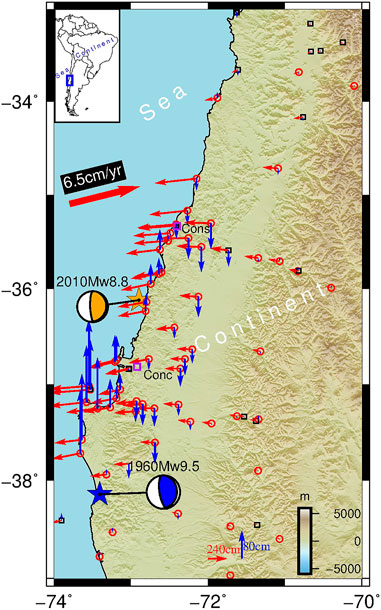
FIGURE 1. The tectonic setting of the 2010 Maule earthquake. The black rectangle represents the continuous GPS stations, and the red circles are campaign stations. The red and blue vectors represent the horizontal and vertical displacements of GPS, respectively. The orange and blue stars are the epicenters of 2010 and 1960 earthquakes, respectively. The orange beach ball is the United States Geological Survey (USGS) centroid moment tensor. The focal mechanism of the blue beach ball is from Fujii and Satake (2013). The bold red arrow shows the interseismic convergence vector between the Nazca plate and the South American plate. The purple rectangles represent the locations of surrounding cities; Cons, Constitución; Conc, Concepción.

The InSAR technique is powerful to detect ground surface displacement, such as earthquakes (Massonnet et al., 1993; Xu et al., 2020; Yang et al., 2020a, 2020b), volcanoes (Guo et al., 2019; Wang L. et al., 2021), and mining collapses (Yang et al., 2016). For the Maule event, the Japan Aerospace Exploration Agency (JAXA) imaged the deformation areas with the Advanced Land Observatory Satellite (ALOS) Phased Array type L-band Synthetic Aperture Radar (PALSAR) images (Tong et al., 2010; Pollitz et al., 2011; Zhang et al., 2021). Besides, this event induced some geohazards such as the tsunami with a maximum runup of 29 m, resulting in 156 casualties and economic losses of about 30000 million dollars (http://www.ngdc.noaa.gov/hazard/tsu.shtml; https://www.ngdc.noaa.gov/hazel/view/hazards/tsunami/event-more-info/4682).

Following the event, different data sources have been used in several studies to investigate the Maule earthquake rupture process and the mechanics of the subduction environment. Tong et al. (2010) quantitatively derived the coseismic slip distribution based on the elastic dislocation model with a combination of GPS and ALOS data. Lay et al. (2010) inferred the finite-fault slip distribution using the teleseismic P, SH, and Rayleigh wave data. Delouis et al. (2010) presented the slip distribution based on the static and High-Rate GPS, teleseismic, and InSAR data. Lorito et al. (2011) derived the slip distribution with a robust model using a combination of tsunami, GPS, InSAR data, and land-level changes (Farías et al., 2010). Luttrell et al. (2011) estimated the stress drop and crustal tectonic stress of the Maule earthquake. However, there is still no research on the coseismic three-dimensional surface displacement field related to this event. Although InSAR has played a significant role in measuring surface deformation, it is confined to one-dimensional line of sight (LOS) displacement of the geohazards such as earthquakes and volcanic eruptions (Jung and Hong, 2017; He et al., 2018; Xiong et al., 2020). The LOS results cannot fully reflect the real deformation in most cases (Song et al., 2017). However, the three-dimensional displacement field can assist us to comprehensively understand the characteristics of the seismogenic fault and provide enlightenment of the earthquake rupture (Fialko et al., 2001; He et al., 2018, 2019; Zhou et al., 2018; Liu et al., 2019; Xiong et al., 2020).

It is well known that GPS data offer high precision in measuring surface deformation, but provide sparse three-dimensional displacement caused by an earthquake. Moreover, the sites of the network of GPS stations registering the Maule earthquake are unevenly distributed, being denser near the coast and more scattered at the epicentral or far-field areas (Hill et al., 2012; Jiang, 2014; Elliott et al., 2016). Therefore, compared to one-dimensional LOS displacement or sparse GPS observations, the large-scale three-dimensional displacement field can provide exhaustive information that helps to produce a straightforward geological interpretation (Jung and Hong, 2017; He et al., 2019). Generally, GPS and InSAR data are fused to estimate three-dimensional surface displacement. As a first step in previous studies (Gudmundsson et al., 2002; Samsonov and Tiampo, 2006; Hu et al., 2012), sparse GPS measurements are interpolated to fill in the LOS grid. To avoid GPS interpolation and consider the spatial correlation of surface displacements among the adjacent points, Guglielmino et al. (2011) proposed the SISTEM method. Based on the elastic theory, SISTEM method can provide the solutions of the strain tensor, the displacement field, and the rigid body rotation tensor. Luo and Chen (2016) proposed the ESISTEM approach that both surrounding InSAR and GPS measurements available were used to constrain the derived displacements, while the SISTEM approach only used the surrounding GPS measurements. Furthermore, neither the SISTEM nor ESISTEM methods account for the relative weight between GPS and InSAR measurements needed to compensate for the highly larger amount of InSAR observations. With the spatial correlation of the adjacent points’ displacements taken into consideration in the SISTEM/ESISTEM methods, more measurements are involved to estimate displacements and strain at the points of interest. Thus, providing a chance to use the variance component estimation (VCE) algorithm to determine accurate relative weights between GPS, ascending, and descending InSAR data in the SISTEM/ESISTEM methods. In previous research, Hu et al. (2012) introduced the VCE algorithm to estimate the relative weight between InSAR and GPS measurements for inferring the three-dimensional surface displacements. However, their method does not consider the spatial correlation of neighboring surface displacements. Liu et al. (2018, 2019) and Hu et al. (2021) incorporated the VCE algorithm into the strain model based on the elastic theory, using only InSAR measurements. Nevertheless, they calculated displacements/strain in a given spatial window, without determining the distance-decaying constant. However, the spatial distribution characteristics and resolutions (spatial scales) of GPS and InSAR data are quite different. For instance, while InSAR observations are homogenously distributed over a broad area, the spatial distribution of the GPS stations is highly heterogeneous in the large-scale deformation area of the 2010 Maule earthquake. Therefore, Liu et al. (2018), Liu et al. (2019) and Hu et al. (2021) approaches are not suitable when integrating GPS and InSAR data to derive the three-dimensional displacement field. In addition, Wang Y. et al. (2021) integrated the VCE and the SISTEM methods to derive three-dimensional surface displacement. However, they defined the relative weight between horizontal and vertical components of GPS data without acknowledging their uncertainties. Moreover, they defined the same distance–decaying constants to multi-source data, which is also not appropriate for GPS and InSAR data with intrinsically different spatial distributions. As a example, for the 2010 Maule earthquake, the spatial scale of GPS data is larger than that of InSAR observations.

To overcome the shortcomings mentioned above, we propose the improved ESISTEM method combined with VCE algorithm (ESISTEM-VCE). We also called this method tight integration of GPS/InSAR data, which is similar to the integration of GPS/INS in navigation. The main objectives of this method are: 1) to avoid the interpolation of sparse GPS data and construct a functional model with physical meaning that takes into account the spatial correlation among adjacent points based on elastic theory; 2) to utilize the uncertainties of horizontal and vertical directions from GPS data, and fully consider the differences of the spatial scales intrinsic to data from GPS networks and InSAR scenery; 3) to make a posteriori estimation of the adjustment stochastic model and determine the accurate weights of GPS, ascending, and descending InSAR data by applying the VCE algorithm. Thus, exploit the intrinsic complementarity of GPS and InSAR data to determine surface displacements. For validation, the improved ESISTEM-VCE method is used to derive the three-dimensional displacements with a simulated experiment. Then, as a novelty, we apply our proposed methodology to the case study of the 2010 Mw 8.8 Maule earthquake.

ESISTEM-VCE method

For an arbitrary point $P^0$, whose position and three-dimensional displacements are $x^0=\left(x_e^0,x_n^0,x_u^0\right)$ and $d^0=\left(d_e^0,d_n^0,d_u^0\right)$, respectively. There are N reference points (RPs) surrounding the $P^0$ with the positions and displacements are $x^i=\left(x_e^i,x_n^i,x_u^i\right)$ and $d^i=\left(d_e^i,d_n^i,d_u^i\right)$, respectively, where $i=\mathrm{1,2},\cdots N$. The subscripts $e$, $n$ and $u$ represent the east-west (E-W), north-south (N-S), and vertical (U) components, respectively. Based on the elastic theory (Guglielmino et al., 2011), the relationship between the displacements $d^0$ and $d^i$ can be expressed as

$d^i=\mathit{H}\mathrm{\Delta }\mathit{x}+d^0(1)$

where $\mathrm{\Delta }x=x^i-x^0={\left[\begin{array}{ccc}\mathrm{\Delta }{x}_e^i& \mathrm{\Delta }{x}_n^i& \mathrm{\Delta }{x}_u^i\end{array}\right]}^{\text{T}}$ denotes the vector distance between the ith RP and the arbitrary point $P^0$, $\mathit{H}=\partial d^i/\partial x^i$ denotes the elements of the displacement gradient tensor. In the SISTEM method, Guglielmino et al. (2011) only used surrounding GPS measurements. Thus, Luo and Chen (2016) proposed the ESISTEM method, where both surrounding GPS and InSAR measurements can be used in deriving displacements. The linear equation for the ESISTEM method can be expressed as

$\mathit{d=AX+e}(2)$

where $\mathit{d}$ is the column observation vector, $\mathit{A}$ is the design matrix, $\mathit{X}$ is the column vector of unknown parameters, and $\mathit{e}$ is the observation error vector. The expressions of the vectors or matrices are shown in the Appendix A. The detailed information about formula derivation can be referred to Luo and Chen (2016).

For the 2010 Mw 8.8 Maule earthquake, the GPS, ascending, and descending InSAR measurements can be together used to extract the three-dimensional surface deformation field. Therefore, the data sets are divided into three groups based on their properties. Their observations are ${\mathit{d}}_{\mathrm{1}}$, ${\mathit{d}}_2$, and ${\mathit{d}}_3$ for GPS, ascending, and descending InSAR measurements, respectively. The corresponding coefficient matrices are ${\mathit{A}}_1$, ${\mathit{A}}_2$, and ${\mathit{A}}_3$, respectively.

The weight matrices ${\mathit{W}}_j$ ($j=\mathrm{1,2,3}$) is determined by $1/{\delta }_j^2$, and ${\delta }_j$ denote the standard deviations of the measurements, with their uncertainties of the GPS as well as InSAR data are utilized, respectively, which is different from Wang Y. et al. (2021). Meanwhile, the estimation for any point of interest can be performed over the RPs with a suitable weighting strategy to automatically lower the contribution of points distant from the point of interest (Pesci and Teza, 2007). Hence, the weighted ${\mathbf{W}}_{\mathit{j}}^{\prime }$ is given as (Shen et al., 1996; Guglielmino et al., 2011)

${\mathit{W}}_{\mathit{j}}^{\prime }={\mathit{W}}_j\exp \left(-d_n/d_j\right)(3)$

where $d_n$ is the distance between the $ith$ RP and the point of interest $P^0$, and $d_j$ are distance–decaying constants for GPS, ascending, and descending InSAR measurements, respectively (Guglielmino et al., 2011), which is evaluated with the following empirical formula:

$d_j=\frac{1}{PQ}{\displaystyle \sum _{p=1}^P{\displaystyle \sum _{q\in K_i}{d}_{pq}}}(4)$

which takes into account the obvious spatial scale differences among different data sets and shows the other main difference from Wang Y. et al. (2021). As Guglielmino et al. (2011) described in the paper, P is the number of the RPs of the network, $K_i$ is the set of Q nearest stations in the circle centered at the i station for different data sets. In our study, we also refer to it that Q ranges between four and six.

Let ${\mathit{N}}_{\mathit{j}}\mathit{=}{\mathit{A}}_{\mathit{j}}^{\mathit{T}}{\mathit{W}}_{\mathit{j}}^{\prime }{\mathit{A}}_{\mathit{j}}$, ${\mathit{L}}_j={\mathit{A}}_j^T{\mathit{W}}_{\mathit{j}}^{\prime }{\mathit{d}}_j$ and $\mathit{N}={\sum }_1^3{\mathit{N}}_j$, $\mathit{L}={\sum }_1^3{\mathit{L}}_j$. With the weighted least square method (WLS) (He et al., 2018; Wang and Gu, 2020), the estimated unknown vector $\widehat{\mathit{X}}$ can be solved, as shown in Eq. 5.

$\stackrel{\mathrm{\wedge }}{\mathit{X}}\mathbf{=}{\mathit{N}}^{\mathrm{-1}}\mathit{L}(5)$

In this paper, we assumed the initial variances for the data sets are ${\sigma }_{01}^2$, ${\sigma }_{02}^2$, and ${\sigma }_{03}^2$, respectively. The relationship between the estimates and the residuals sum of squares (RSS) of observations is (Cui et al., 2001; Xu et al., 2009)

$\mathit{S}\mathit{\theta =}{\mathit{W}}_{\mathit{\theta }}(6)$

and

$\mathbf{S}=\left[\begin{array}{ccc}3\ast n1-2\mathit{tr}\left({\mathit{N}}^{-1}{\mathit{N}}_1\right)+tr{\left({\mathit{N}}^{-1}{\mathit{N}}_1\right)}^2& \mathit{tr}\left({\mathit{N}}^{-1}{\mathit{N}}_1{\mathit{N}}^{-1}{\mathit{N}}_2\right)& \mathit{tr}\left({\mathit{N}}^{-1}{\mathit{N}}_1{\mathit{N}}^{-1}{\mathit{N}}_3\right)\\ \mathit{tr}\left({\mathit{N}}^{-1}{\mathit{N}}_1{\mathit{N}}^{-1}{\mathit{N}}_2\right)& n2-2\mathit{tr}\left({\mathit{N}}^{-1}{\mathit{N}}_2\right)+\mathit{tr}{\left({\mathit{N}}^{-1}{\mathit{N}}_2\right)}^2& \mathit{tr}\left({\mathit{N}}^{-1}{\mathit{N}}_2{\mathit{N}}^{-1}{\mathit{N}}_3\right)\\ \mathit{tr}\left({\mathit{N}}^{-1}{\mathit{N}}_1{\mathit{N}}^{-1}{\mathit{N}}_3\right)& \mathit{tr}\left({\mathit{N}}^{-1}{\mathit{N}}_2{\mathit{N}}^{-1}{\mathit{N}}_3\right)& n3-2tr\left({\mathit{N}}^{-1}{\mathit{N}}_3\right)+\mathit{tr}{\left({\mathit{N}}^{-1}{\mathit{N}}_3\right)}^2\end{array}\right]$

$\widehat{\mathit{\theta }}={\left[\begin{array}{ccc}{\widehat{\sigma }}_{01}^2& {\widehat{\sigma }}_{02}^2& {\widehat{\sigma }}_{03}^2\end{array}\right]}^T$, ${\mathit{W}}_{\mathbf{\theta }}\mathbf{=}{\left[\begin{array}{ccc}{\mathit{V}}_{\mathrm{1}}^{\mathit{T}}{\mathit{W}}_{\mathrm{1}}^{\prime }{\mathit{V}}_{\mathrm{1}}& {\mathit{V}}_{\mathrm{2}}^{\mathit{T}}{\mathit{W}}_{\mathrm{2}}^{\prime }{\mathit{V}}_{\mathrm{2}}& {\mathit{V}}_{\mathrm{3}}^{\mathit{T}}{\mathit{W}}_{\mathrm{3}}^{\prime }{\mathit{V}}_{\mathrm{3}}\end{array}\right]}^{\mathit{T}}$, where $n_1$, $n_2$, and $n_3$ are the numbers of the GPS measurements, ascending, and descending ALOS InSAR results. The solution of Eq. 6 can be expressed as

$\widehat{\mathit{\theta }}={\mathit{S}}^{-1}{\mathit{W}}_{\theta }(7)$

In a real application, iteration is needed to obtain an accurate solution by adjusting the weight as follows:

${\mathit{W}}_{\mathit{j}}^{\prime }{}^{\mathit{k}}=\frac{c}{{\widehat{\sigma }}_{0j}^2}{\mathit{W}}_{\mathit{j}}^{\prime }{}^{\mathit{k}-1},\left(j=\mathrm{1,2,3}\right)(8)$

where $c$ is an arbitrary positive constant, which usually can be assumed to be ${\widehat{\sigma }}_{01}^2$. The iteration will not stop until the variance components are almost identical, i.e. ${\widehat{\sigma }}_{01}^2\approx {\widehat{\sigma }}_{02}^2\approx {\widehat{\sigma }}_{03}^2$. In the final, the weights from the last iteration are used to determine the optimal three-dimensional surface displacement field with Eq. 5.

Figure 2 shows the flowchart of the ESISTEM-VCE method. The main steps of the proposed method are as follows. S0: Give the studied region that the three-dimensional surface displacement field needs to be solved. S1: Give the GPS, ascending, and descending InSAR measurements, and divide them into three groups. S2: Determine the $d_j$ according to formula in Guglielmino et al. (2011) with Eq. 4, and compute the ${\mathit{W}}_{\mathit{j}}$ ($j=\mathrm{1,2,3}$) according to their standard deviations. S3: Use Eq. 3 to compute the weighted ${\mathit{W}}_{\mathit{j}}^{\prime }$ of the RPs. S4: Compute the estimated unknown vector with Eq. 5. S5: Compute the variance components ${\widehat{\sigma }}_{0j}^2$, ($j=\mathrm{1,2,3}$) with Eq. 7. S6: Use Eq. 8 to update the weight matrix ${\mathit{W}}_{\mathit{j}}^{\prime }$, ($j=\mathrm{1,2,3}$) and go to S4. If ${\widehat{\sigma }}_{01}^2\approx {\widehat{\sigma }}_{02}^2\approx {\widehat{\sigma }}_{03}^2$, terminate the iteration. S7: Determine the optimal three-dimensional surface displacement with Eq. 5. S8: Go to S0 until the points in the studied area are all solved.

FIGURE 2

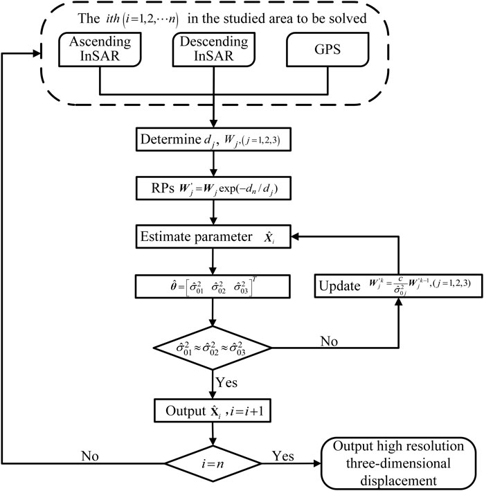
FIGURE 2. The flowchart of the ESISTEM-VCE method.

Simulation experiments

The ESISTEM-VCE method is tested and compared with the ESISTEM method by simulation experiments. The simulated LOS and GPS displacements are obtained from the three-dimensional surface displacement under a given fault slip based on the elastic half-space dislocation theory (Okada, 1985). The model parameters are shown in Table 1, and the slip distribution is shown in Figure 3A. Figures 3B–D show the three-dimensional surface displacement with a cell size of 5 km × 5 km. Two InSAR LOS displacements are calculated from the simulated three-dimensional displacement field with mean unit vectors, [−0.6058, −0.1776, 0.7753] and [0.5855, −0.1697, 0.7919] for ascending and descending ALOS LOS measurements, respectively, based on the InSAR data for the 2010 earthquake (Figures 3E,F). The spatially correlated noises with 1 cm standard deviation on a scale length of 10 km are added to the LOS displacements (Lohman and Simons, 2005; Luo and Chen, 2016). The black dots in Figure 3B are the selected points that are assumed to be GPS stations, and unbiassed Gaussian noises with standard deviations of 3 and 5 mm are added to the horizontal and vertical displacements, respectively.

TABLE 1

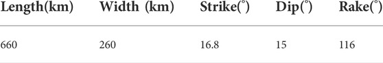
TABLE 1. Model parameters in the experiments.

FIGURE 3

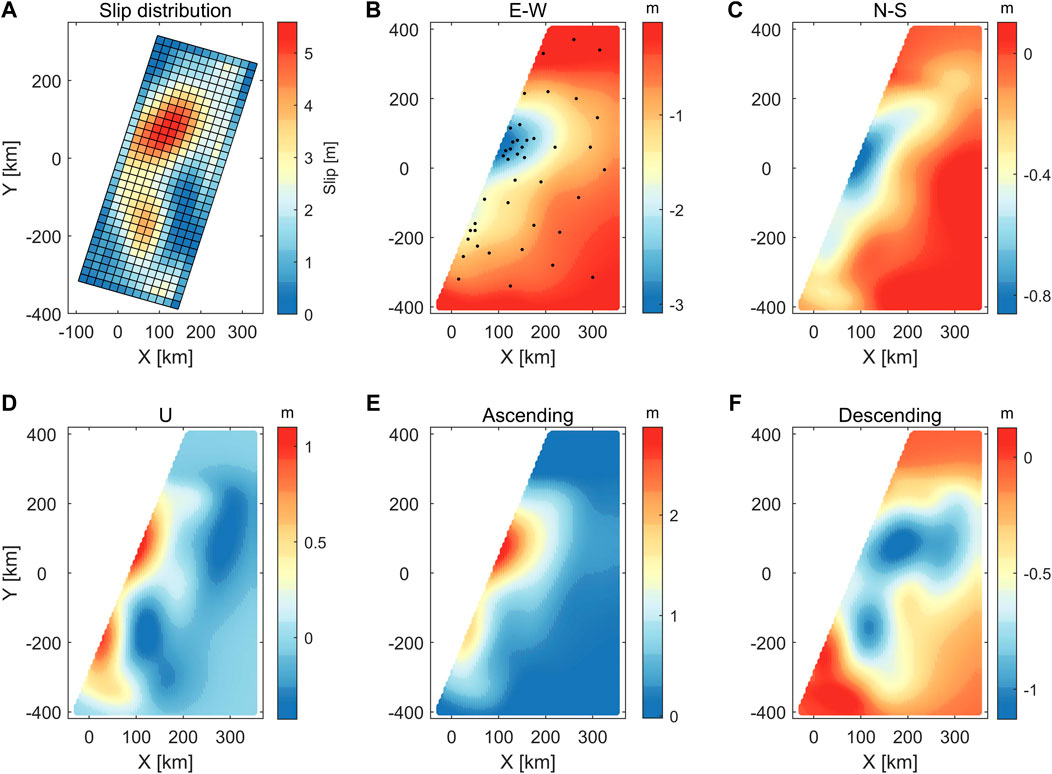
FIGURE 3. The simulated data used in the simulation experiments. (A) The slip distribution. (B–D) The simulated three-dimensional displacement field according to the elastic half-space dislocation theory. (E,F) The simulated ascending and descending InSAR displacements.

Figure 4 shows the average three-dimensional displacement fields of 400 tests, which are obtained by Monte Carlo simulation using the ESISTEM-VCE and ESISTEM methods, respectively. It can be found that the derived displacements are both consistent with the simulated ones. However, the displacements of E-W and U components from the ESISTEM method are underestimated. The results from the ESISTEM-VCE method are closer to the simulated values and smoother than those from ESISTEM method in three components.

FIGURE 4

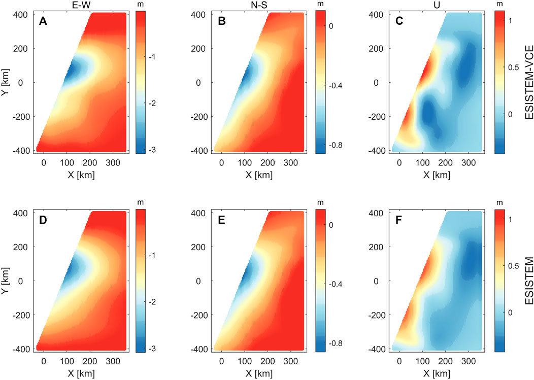
FIGURE 4. Solutions of ESISTEM-VCE and ESISTEM methods for simulation example. The upper row (A-C) is from the ESISTEM-VCE method, the low row (D-F)is from the ESISTEM method.

To quantitatively evaluate the performance of both methods, we use the root mean square error (RMSE)

$RMSE=\sqrt{{[X_{sub}-{\widehat{X}}_{sub}]}^2/num}\left(sub=e,n,u\right)(9)$

where num is the total number of points, $X_{sub}$ are the simulated displacements in three components, and ${\widehat{X}}_{sub}$ are the derived ones from the ESISTEM-VCE and ESISTEM methods.

Table 2 shows the average RMSEs in three components from different methods. Meanwhile, Figure 5 displays the RMSEs for 400 tests. As expected, the RMSEs of the three-dimensional displacements from the ESISTEM-VCE method are lower than those from the ESISTEM method. Compared with the ESISTEM method, the ESISTEM-VCE method achieves 97.1%, 3.9%, and 84% improvements in three components, respectively. It is obvious that the RMSE of the N-S component is larger than those of the E-W and U components, and the accuracy and improvement are worse than the other two components. This is mainly because the LOS displacement is not sensitive to the north-south direction, and the N-S displacement is mainly constrained by the GPS data.

TABLE 2

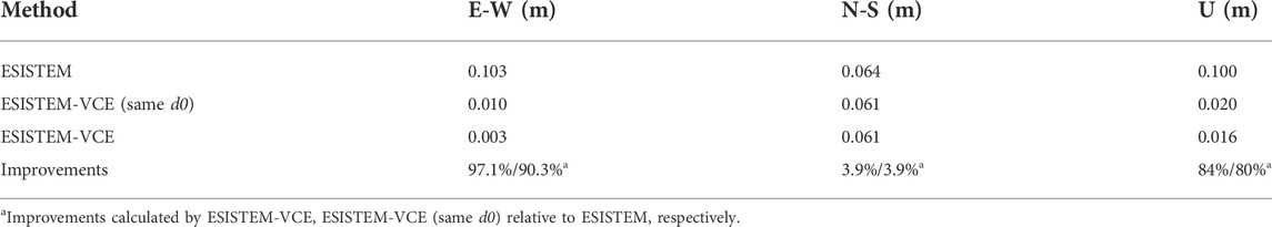
TABLE 2. The RMSEs for the EISISTEM-VCE and ESISTEM methods.

FIGURE 5

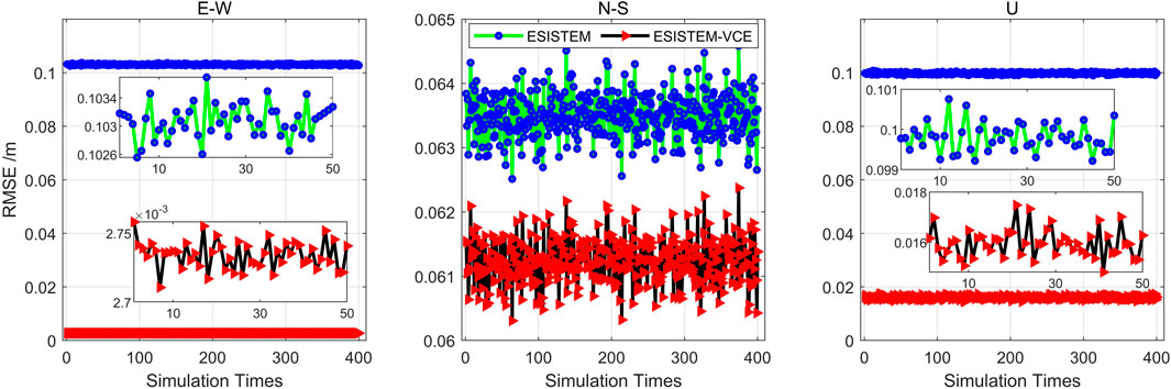
FIGURE 5. The RMSEs for three components from ESISTEM-VCE and ESISTEM methods with 400 Monte Carlo simulations. The black and green lines represent the RMSEs of the ESISTEM-VCE and ESISTEM methods, respectively. The subfigures in E-W and U components are partial enlarged view, respectively.

Furthermore, we assumed that the distance–decaying constants for the ascending and descending InSAR measurements are the same as that of GPS measurements in the ESISTEM-VCE method, which is named ESISTEM-VCE (same d0) method. This method is used to compare and verify the significance of the different d0 for different data sets that differ in their spatial scales. The RMSEs are also listed in Table 2, and the improvements are slightly lower than those of ESISTEM-VCE method, which shows that the ESISTEM-VCE performs best. Since the spatial scales of GPS, ascending, and descending InSAR data are different, it is critical to give them different distance–decaying constants, which can be supported by the improvements.

For the ESISTEM-VCE method, the number of RPs is vital for the accuracy of the method. A random Monte Carlo simulation with RPs ranging from 10 to 150 was carried out to assess the performances of the ESISTEM-VCE method. The behavior of the RMSEs versus the number of RPs is reported in Figure 6. As expected, it is possible to see that the RMSEs of all three components decrease (the accuracies of the methods increase) with the increase of RPs and tend to be flat. The RMSEs of the N-S component are also greater than the other two components, which is consistent with the performance of Figure 5. Additionally, Figure 6 suggests that, in our simulation experiments, a good tradeoff between the accuracies and the number of RPs can be obtained with 50–60 RPs.

FIGURE 6

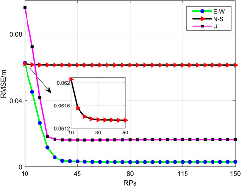
FIGURE 6. The accuracies (RMSEs) versu the RPs.

Three-Dimensional displacement field of the 2010Mw 8.8 Maule earthquake

GPS and InSAR data

We assembled a database of GPS and InSAR observations to extract the three-dimensional displacement field of the 2010 Mw 8.8 Maule earthquake (Figure 7). The GPS data were obtained from Tong et al. (2010), Delouis et al. (2010), Vigny et al. (2011), Moreno et al. (2012), and Melnick et al. (2013). There are 77 stations in total (Figure 7A). The GPS data available prior to the 27th February 2010 Maule earthquake were collected at different times before and re-observed within a few days to months after the event. They were observed on existing benchmarks installed in the framework of the South American Geodynamic Activities (SAGA) project, Central Andes GPS Project (CAP), Concepción Geodetic Activities (COGA) project (Bevis et al., 2001; Klotz et al., 2001; Moreno et al., 2011). These GPS data were processed with the GAMIT/GLOCK software (King and Bock, 2000; Herring et al., 2009) and Bernese GPS software V5.0 (Dach et al., 2007) to estimate the coseismic displacement at each station affected by the Maule earthquake. Detailed information on data acquisition and processing can be found in the references above.

FIGURE 7

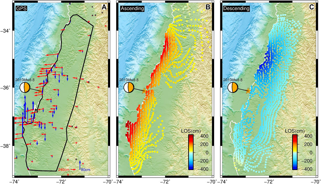
FIGURE 7. The distribution of the data set used in this study. (A) The GPS data; the black line denotes the area of three-dimensional displacement to be estimated. (B) The ascending ALOS LOS displacements. (C) The descending ALOS LOS displacements.

The ALOS data were from Tong et al. (2010). Nine tracks (T111-T119) of ascending InSAR data were obtained with the Fine Beam Single Polarization (FBS) strip-mode (Figure 7B). Two tracks of descending data were obtained with two subswaths (T422-subswaths 3–4) of Scanning Synthetic Aperture Radar (ScanSAR) mode and ScanSAR-FBS mode, and one track (T420) of FBS-FBS mode (Tong et al., 2010) (Figure 7C). The various mode SAR data were processed by using the FBS to ScanSAR software and ScanSAR-ScanSAR processor (Tong et al., 2010) of GMTSAR software (Sandwell et al., 2008). The unwrapped interferograms were converted into LOS displacements composed of 820 and 1112 data points for ascending (the maximum displacement is 418 cm) and descending InSAR observations (the maximum negative displacement is 374 cm), respectively, which are available at ftp://topex.ucsd.edu/pub/chile_eq/. The more detailed information can be referred to Tong et al. (2010).

Results and discussions

Figures 8A–F show the three-dimensional surface displacement fields for the Maule earthquake with GPS and InSAR data derived from ESISTEM-VCE and ESISTEM methods. The derived displacement field is in the hanging wall of the ruptured fault that occurs on the subduction interface, whose strike angle is N16.8°E according to Tong et al. (2010).

FIGURE 8

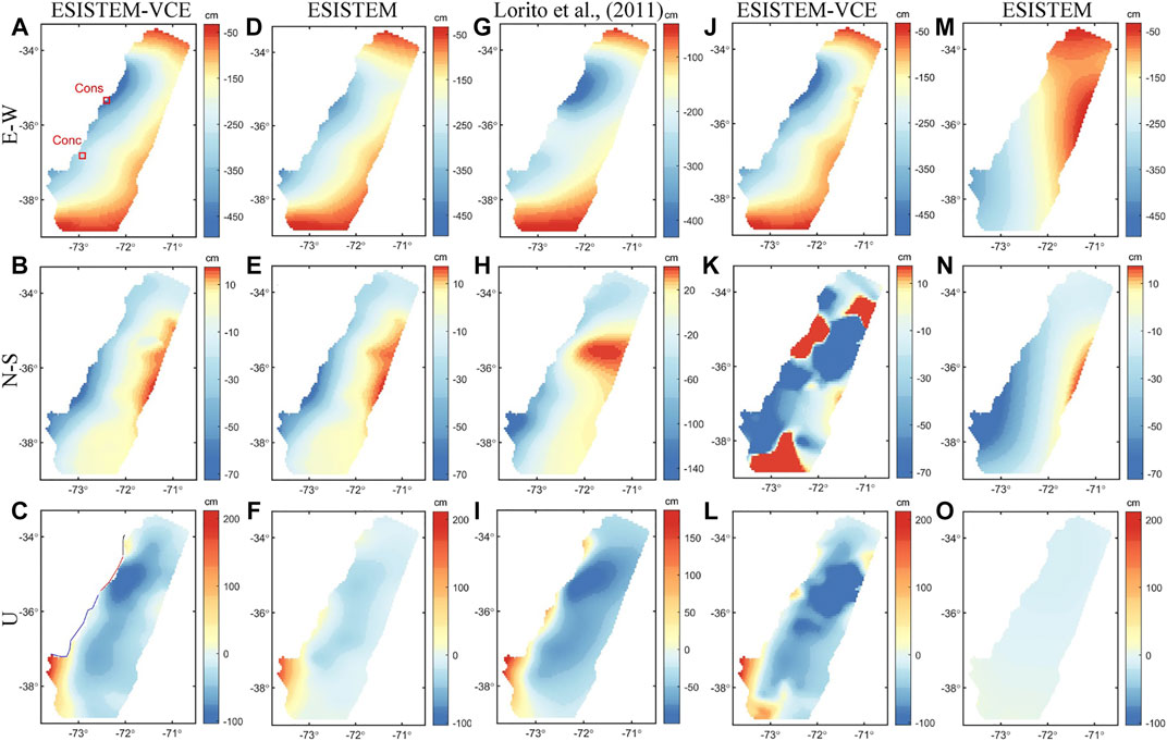
FIGURE 8. Three-dimensional surface displacement field derived from different data sources. (A–C) Three-dimensional surface displacement field derived from the ESISTEM-VCE method with all data. In (A), the red rectangles denote the locations of surrounding cities. (D–F) Three-dimensional surface displacement field derived from the ESISTEM method with all data. (G–I) Three-dimensional displacement field from forward modeling with the slip distribution model from Lorito et al. (2011). (J–L) Three-dimensional displacement field derived from the continuous GPS and LOS data with the ESISTEM-VCE method. (M–O) Three-dimensional displacement field derived from the continuous GPS and LOS data with the ESISTEM method.

Figure 8A shows that the E-W displacement is dominated by the seaward movement. The most intense deformation zone is located to the north of the epicenter, with a maximum value of 495.5 cm near the city of Constitución. The other significant deformation zone is located to the south of the epicenter, with a maximum value of 396.2 cm. These two locations are generally consistent with the large LOS displacements of the corresponding regions in Figures 7B,C. Meanwhile, these maximum value areas display that this event ruptured along the north and south directions, which are consistent with the significant coseismic slip areas in published slip models (e.g., Tong et al., 2010; Vigny et al., 2011; Lin et al., 2013).

Compared to the E-W deformation, the magnitude of the N-S deformation (Figure 8B) is significantly small, and the spatial distribution is different from the E-W component. For example, the most significant deformation of N-S is located around the epicenter, while that of E-W is at the north of the epicenter. The displacement along the coastline moves southward, with a maximum displacement of 72.5 cm, while that away from the coastline moves northward.

The vertical displacement (Figure 8C) demonstrates that the overall magnitude of displacement is smaller than that in the E-W component. The displacement ranges from −103.8 to 211.8 cm, and the maximum surface uplift is located south of the epicenter. Along the coastline, the displacement can be roughly divided into three areas, the areas corresponding to the black, red, and blue lines, which is consistent with the results of Vigny et al. (2011). The north (corresponding to the black line) and south (corresponding to the blue line) areas show the surface uplift. The zone of the epicenter reveals the uplift with displacement lower than 50 cm, which can not be reflected from the sparse GPS or InSAR observations alone. Vigny et al. (2011) described that the data near the epicenter of blue lines (−36.7° to −35.8°) are scarce or lacking. Combined with the GPS data, InSAR observations could detect more deformation information that can not be obtained by a single data source. This implies that the InSAR data can better complement the GPS data in the extraction of three-dimensional displacement.

Figures 8D–F present the three-dimensional surface displacement field from the ESISTEM method. It is noticeable that the deformation characteristics are similar to those of the ESISTEM-VCE method. However, the magnitude of the vertical displacements is underestimated especially in the north or south of the epicenter, which is consistent with the situation in the simulation examples. This should be attributed to the inaccurate weight ratio among the GPS, ascending, and descending ALOS InSAR data.

To verify that the vertical displacement is underestimated and to assess the accuracy of our methods quantitatively, we compared the derived displacements to the land-level changes estimated through observations of bleached lithothamnioids crustose coralline algae, submerged quays and piers and flooded beaches, flooded river bars with submerged and flooded trees, and swampy vegetation (Vargas et al., 2011). Figure 9 shows the comparison among the vertical displacements from the field investigation, the ESISTEM-VCE, and the ESISTEM methods, with their corresponding uncertainties also given. It shows that the displacements from the ESISTEM-VCE method are closer to the field investigations than those from ESISTEM method. The overall uncertainties of the ESISTEM-VCE method are smaller than those of ESISTEM method. We obtained the RMSEs between the derived vertical displacements and field investigations, and they are 32.1 and 44.5 cm for ESISTEM-VCE and ESISTEM methods, respectively. Compared to the ESISTEM method, an improvement of 27.9% is achieved by the ESISTEM-VCE method, which should be attributed to the more accurate variance and weight estimations of the InSAR and GPS measurements.

FIGURE 9

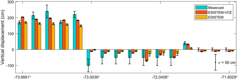
FIGURE 9. Comparison among the vertical displacements measured from field investigation, derived from the ESISTEM-VCE and the ESISTEM methods. The error bars denote the $2\sigma$ uncertainties.

The reliability of the three-dimensional displacement field obtained by the ESISTEM-VCE method is further verified. The slip distribution model given by Lorito et al. (2011) is used to obtain the three-dimensional displacement field from forward modeling (Figures 8G–I). Compared to Figures 8A–C, we found that the deformation patterns are consistent with each other near the epicenter and along the coastline. Whereas, in the area distant from the coastline, they show some differences, especially in the N-S component. These differences may be due to different data constraints and methods used. The results of Figures 8G–I are derived from the forward modeling with the slip distribution based on the elastic dislocation theory, in which the fault plane is divided into 200 subfaults of 25 × 25 km with a large scale. Nevertheless, the similar deformation patterns suggest that the derived results from GPS and InSAR data using the ESISTEM-VCE method are reasonable.

The abundant independent observations are helpful to extract the accurate and detailed three-dimensional deformation field. We collected the continuous and campaign GPS data in this study. As is known to us that the precision of the continuous GPS data is higher than the campaign ones. To highlight the importance of campaign GPS data, we retrieved the three-dimensional deformations only with the continuous GPS data and LOS measurements using the ESISTEM-VCE (Figures 8J–L) and ESISTEM (Figures 8M–O) methods. Figures 8A–F,J–O show that the magnitudes and characteristics of deformation are quite different, especially in the N-S components. This should be related to that a few continuous GPS stations can not sufficiently provide constraints on the magnitude and trend of deformation and cannot make up for the insensitivity of LOS measurements to the north-south component. However, it is observed that the magnitudes of displacements in Figures 8J,L are closer to Figures 8A,C than those in Figures 8M,O. This demonstrates that the VCE method is still capable of determining the accurate relative weights between GPS and ALOS data sets. It also manifests that the N-S displacement is mostly constrained by the GPS observations, and the campaign GPS observations play a dominant role in the reconstruction of precise three-dimensional surface deformation.

In addition, the three-dimensional displacement field derived from the ESISTEM-VCE (same d0) method is shown in Figure 10, with the distance-decaying constants for ascending and descending InSAR measurements are same as that of GPS data. Figure 10 shows a deformation pattern similar to Figures 8A–C. The RMSE between the vertical displacements from ESISTEM-VCE (same d0) and the field investigations is also obtained, which is 35.2 cm. Compared with ESISTEM method, 20.9% improvement is achieved. The comparisons of 27.9 and 20.9% show that the distance–decaying constants of different data sets should be considered. This also implies that the ESISTEM-VCE method is effective.

FIGURE 10

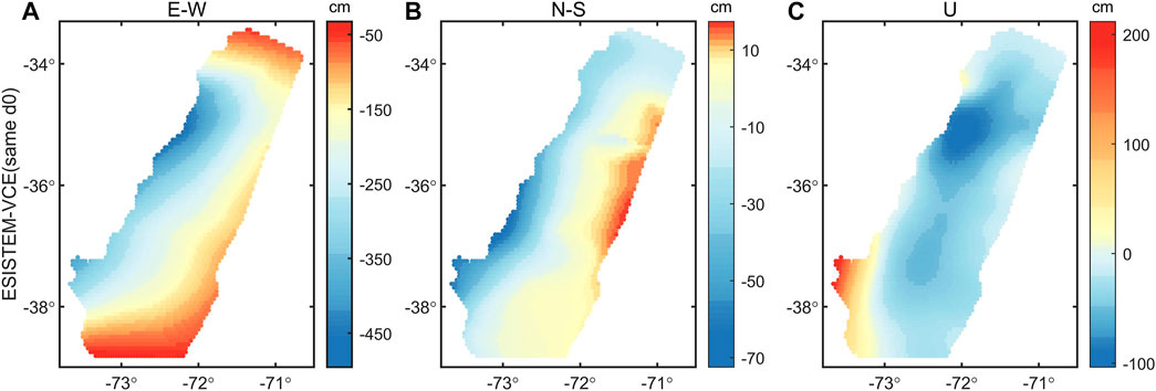
FIGURE 10. Three-dimensional surface displacement field derived from the ESISTEM-VCE method with the same distance–decaying constants for GPS and InSAR data. (A) The east-west displacement. (B) The north-south displacement. (C) The vertical displacement.

The predominantly westward horizontal motion reveals that there existed the right-lateral strike-slip component in the main rupture region, with the east-west extrusion and north-south dextral shear. Meanwhile, it shows that the rupture of this event was bilateral, and propagated to north and south from the epicenter (Lay et al., 2010; Koper et al., 2012; Yue et al., 2014). The case of predominantly east-west displacement could also occur in large subduction zones, such as South America, Japan, or Cascadia (Grandin et al., 2016). A few minutes after the Maule earthquake, large tsunami waves hit the coast ranging from about −39° to −33° (Figure 1). The localized maximum runup of 29 m is located at Constitución, and the runup distribution exhibited almost a decaying trend along the north with runup heights typically of 5–10 m (Fritz et al., 2011; Vargas et al., 2011). The magnitude of displacement decreases from Constitución to the north in the E-W component, showing a similar trend. The predominant deformation in the vertical component along the coastline shows an uplift pattern. These characteristics are coherent with the observations from bleached lithothamnioids crustose coralline algae (Vargas et al., 2011) (Figure 9). The three-dimensional displacement could provide insights into the motion of the tsunami from the similar decaying trend, and be used to make up for insufficient spatial resolution of the coastal uplift measured from bleached lithothamnioids crustose coralline algae or GPS stations.

Conclusion

The three-dimensional displacement field is significant for understanding the characteristics of the seismogenic fault by providing enlightenment of the earthquake rupture. This study develops an improved ESISTEM-VCE method, which is a tight integration of GPS and InSAR data, to derive the three-dimensional displacement field. On one hand, the ESISTEM-VCE method can exploit the spatial correlation of the displacement among adjacent points and determine accurate relative weights between different data sets. On the other hand, the ESISTEM-VCE method can take full advantage of the information about the precision of the GPS measurements and the differences of the spatial scales for different data sets. Thus, the ESISTEM-VCE method can be applied to derive the three-dimensional displacement associated with a transient event such as an earthquake. Simulated experiments are firstly carried out to validate the method. Then, the accurate coseismic three-dimensional displacement field of the 2010 Mw 8.8 Maule earthquake is successfully retrieved for the first time by a combination of GPS and InSAR data. The comparison with the land-level changes from the field investigation also validates that the ESISTEM-VCE method is feasible and valid.

Data availability statement

The original contributions presented in the study are included in the article/Supplementary Material, further inquiries can be directed to the corresponding author.

Author contributions

LX: Investigation, writing-original draft, writing-review and editing, final approval of the version to be submitted. CX: Conceptualization, methodology, supervision, writing-review and editing, funding acquisition, final approval of the version to be submitted. YL: Conceptualization, formal analysis, writing-review and editing, funding acquisition, final approval of the version to be submitted. YZ: Writing-review and editing, final approval of the version to be submitted. JG: Writing-review and editing, final approval of the version to be submitted. FO-C: Writing-review and editing, final approval of the version to be submitted.

Funding

This work is co-supported by the National Natural Science Foundation of China (No. 41721003, No. 41861134009, and No. 41874011), the National Key Research Development Program of China (Grant No. 2018YFC1503603), and PCI PII-180003 ANID-Chile.

Conflict of interest

The authors declare that the research was conducted in the absence of any commercial or financial relationships that could be construed as a potential conflict of interest.

Publisher’s note

All claims expressed in this article are solely those of the authors and do not necessarily represent those of their affiliated organizations, or those of the publisher, the editors and the reviewers. Any product that may be evaluated in this article, or claim that may be made by its manufacturer, is not guaranteed or endorsed by the publisher.

Appendix A: The ESISTEM method

The linear equation for the ESISTEM method is

$\mathit{d}\mathrm{=}\mathit{AX}\mathrm{+}\mathit{e}$

where $\mathit{d}$ is the observation vector

$\mathit{d}=\left[\begin{array}{c}{\mathit{d}}_1\\ {\mathit{d}}_2\\ {\mathit{d}}_3\end{array}\right]=\left[\begin{array}{c}{\mathit{d}}_{GPS}\\ {\mathit{d}}_{ASC}\\ {\mathit{d}}_{DES}\end{array}\right]$

and $\mathit{A}$ is the design matrix

$\mathit{A}=\left[\begin{array}{c}{\mathit{A}}_1\\ {\mathit{A}}_2\\ {\mathit{A}}_3\end{array}\right]=\left[\begin{array}{c}{\mathit{A}}_{GPS}\\ {\mathit{S}}_{ASC}{\mathit{A}}_{ASC}\\ {\mathit{S}}_{DES}{\mathit{A}}_{DES}\end{array}\right]$

the matrices forms of the ${\mathit{A}}_{GPS}$, ${\mathit{A}}_{ASC}$, and ${\mathit{A}}_{DES}$ are

${\mathit{A}}_j=\left[\begin{array}{cccccccccccc}1& 0& 0& \mathrm{\Delta }{x}_e^1& \mathrm{\Delta }{x}_n^1& \mathrm{\Delta }{x}_u^1& 0& 0& 0& 0& \mathrm{\Delta }{x}_u^1& -\mathrm{\Delta }{x}_n^1\\ 0& 1& 0& 0& \mathrm{\Delta }{x}_e^1& 0& \mathrm{\Delta }{x}_n^1& \mathrm{\Delta }{x}_u^1& 0& -\mathrm{\Delta }{x}_u^1& 0& \mathrm{\Delta }{x}_e^1\\ 0& 0& 1& 0& 0& \mathrm{\Delta }{x}_e^1& 0& \mathrm{\Delta }{x}_n^1& \mathrm{\Delta }{x}_u^1& \mathrm{\Delta }{x}_n^1& -\mathrm{\Delta }{x}_e^1& 0\\ ⋮& ⋮& ⋮& ⋮& ⋮& ⋮& ⋮& ⋮& ⋮& ⋮& ⋮& ⋮\\ 1& 0& 0& \mathrm{\Delta }{x}_e^N& \mathrm{\Delta }{x}_n^N& \mathrm{\Delta }{x}_u^N& 0& 0& 0& 0& \mathrm{\Delta }{x}_u^N& -\mathrm{\Delta }{x}_n^N\\ 0& 1& 0& 0& \mathrm{\Delta }{x}_e^N& 0& \mathrm{\Delta }{x}_n^N& \mathrm{\Delta }{x}_u^N& 0& -\mathrm{\Delta }{x}_u^N& 0& \mathrm{\Delta }{x}_e^N\\ 0& 0& 1& 0& 0& \mathrm{\Delta }{x}_e^N& 0& \mathrm{\Delta }{x}_n^N& \mathrm{\Delta }{x}_u^N& \mathrm{\Delta }{x}_n^N& -\mathrm{\Delta }{x}_e^N& 0\end{array}\right],\left(j=GPS/ASC/DES\right)$

the ${\mathit{S}}_m\left(m=ASC/DES\right)$ in the matrix $\mathit{A}$ is composed of the projection coefficients that for the ascending/descending InSAR measurements from E-W, N-S, and U components to LOS displacement.

And $\mathit{X}$ is the parameter vector

$\mathit{X}={\left[\begin{array}{cccccccccccc}{d}_e^0& d_n^0& d_u^0& {\epsilon }_{11}& {\epsilon }_{12}& {\epsilon }_{13}& {\epsilon }_{22}& {\epsilon }_{23}& {\epsilon }_{33}& {\omega }_1& {\omega }_2& {\omega }_3\end{array}\right]}^{\text{T}}$

where $\epsilon$ and $\omega$ representing strain tensor and rigid body rotation tensor, respectively.

References

Bevis, M., Kendrick, E., Smalley, R., Brooks, B., Allmendinger, R., and Isacks, B. (2001). On the Strength of Interplate Coupling and the Rate of Back Arc Convergence in the Central Andes: an Analysis of the Interseismic Velocity Field. Geochem. Geophys. Geosyst. 2 (11). doi:10.1029/2001gc000198

CrossRef Full Text | Google Scholar

Cui, X., Yu, Z., Tao, B., Liu, D., Yu, D., Sun, H., et al. (2001). Generalized Surveying Adjustment. 2nd ed Wuhan, China: Wuhan Univ. Press, 102–114.

Google Scholar

Dach, R., Hugentobler, U., Fridez, P., and Meindl, M. (2007). Bernese GPS Software 5.0. Berne, Switzerland: Astron. Inst. Univ. of Berne. available at http://www.bernese.unibe. ch/docs/DOCU50draft.pdf.

Google Scholar

Delouis, B., Nocquet, J. M., and Vallée, M. (2010). Slip Distribution of the February 27, 2010 Mw = 8.8 Maule Earthquake, Central Chile, from Static and High-Rate GPS, InSAR, and Broadband Teleseismic Data. Geophys. Res. Lett. 37, L17305. doi:10.1029/2010GL043899

CrossRef Full Text | Google Scholar

Elliott, J., Jolivet, R., González, P., Avouac, J., Hollingsworth, J., Searle, M., et al. (2016). Himalayan Megathrust Geometry and Relation to Topography Revealed by the Gorkha Earthquake. Nat. Geosci. 9, 174–180. doi:10.1038/ngeo2623

CrossRef Full Text | Google Scholar

Farías, M., Vargas, G., Tassara, A., Carretier, S., Baize, S., Melnick, D., et al. (2010). Land-level Changes Produced by the Mw 8.8 2010 Chilean Earthquake. Science 329 (5994), 916. doi:10.1126/science.1192094

PubMed Abstract | CrossRef Full Text | Google Scholar

Fialko, Y., Simons, M., and Agnew, D. (2001). The Complete (3-D) Surface Displacement Field in the Epicentral Area of the 1999M_W7.1 Hector Mine Earthquake, California, from Space Geodetic Observations. Geophys. Res. Lett. 28 (16), 3063–3066. doi:10.1029/2001gl013174

CrossRef Full Text | Google Scholar

Fritz, H. M., Petroff, C. M., Catalán, P. A., Cienfuegos, R., Winckler, P., Kalligeris, N., et al. (2011). Field Survey of the 27 February 2010 Chile Tsunami. Pure Appl. Geophys. 168 (11), 1989–2010. doi:10.1007/s00024-011-0283-5

CrossRef Full Text | Google Scholar

Fujii, Y., and Satake, K. (2013). Slip Distribution and Seismic Moment of the 2010 and 1960 Chilean Earthquakes Inferred from Tsunami Waveforms and Coastal Geodetic Data. Pure Appl. Geophys. 170 (9–10), 1493–1509. doi:10.1007/s00024-012-0524-2

CrossRef Full Text | Google Scholar

Grandin, R., Klein, E., Métois, M., and Vigny, C. (2016). Three‐dimensional Displacement Field of the 2015M_w8.3 Illapel Earthquake (Chile) from across‐ and Along‐track Sentinel‐1 TOPS Interferometry. Geophys. Res. Lett. 43, 2552–2561. doi:10.1002/2016GL067954

CrossRef Full Text | Google Scholar

Gudmundsson, S., Sigmundsson, M., and Carstensen, J. (2002). Three-dimensional Surface Motion Maps Estimated from Combined Interferometric Synthetic Aperture Radar and GPS Data. J. Geophys. Res. 107 (B10), 2250. doi:10.1029/2001JB000283

CrossRef Full Text | Google Scholar

Guglielmino, F., Nunnari, G., Puglisi, G., and Spata, A. (2011). Simultaneous and Integrated Strain Tensor Estimation from Geodetic and Satellite Deformation Measurements to Obtain Three-Dimensional Displacement Maps. IEEE Trans. Geosci. Remote Sens. 49 (6), 1815–1826. doi:10.1109/tgrs.2010.2103078

CrossRef Full Text | Google Scholar

Guo, Q., Xu, C., Wen, Y., Liu, Y., and Xu, G. (2019). The 2017 Noneruptive Unrest at the Caldera of Cerro Azul Volcano (Galapagos Islands) Revealed by InSAR Observations and Geodetic Modelling. Remote Sens. 11 (17), 1992. doi:10.3390/rs11171992

CrossRef Full Text | Google Scholar

He, P., Wen, Y., Xu, C., and Chen, Y. (2019). Complete Three-Dimensional Near-Field Surface Displacements from Imaging Geodesy Techniques Applied to the 2016 Kumamoto Earthquake. Remote Sens. Environ. 232, 111321. doi:10.1016/j.rse.2019.111321

CrossRef Full Text | Google Scholar

He, P., Wen, Y., Xu, C., and Chen, Y. (2018). High-quality Three-Dimensional Displacement Fields from New-Generation SAR Imagery: Application to the 2017 Ezgeleh, Iran, Earthquake. J. Geod. 93, 573–591. doi:10.1007/s00190-018-1183-6

CrossRef Full Text | Google Scholar

Herring, T. A., King, R. W., and McClusky, S. C. (2009). Documentation of the MIT GPS Analysis Software: GAMIT V 10.35, Mass. Cambridge: Inst. of Technol.

Google Scholar

Hill, E., Borrero, J., Huang, Z., Qiu, Q., Banerjee, P., Natawidjaja, D., et al. (2012). The 2010 Mw 7.8 Mentawai Earthquake: Very Shallow Source of a Rare Tsunami Earthquake Determined from Tsunami Field Survey and Near-Field GPS Data. J. Geophys. Res. 117, B06402. doi:10.1029/2012jb009159

CrossRef Full Text | Google Scholar

Hu, J., Li, Z., Sun, Q., Zhu, J., and Ding, X. (2012). Three-dimensional Surface Displacements from InSAR and GPS Measurements with Variance Component Estimation. IEEE Geosci. Remote Sens. Lett. 9 (4), 754–758. doi:10.1109/LGRS.2011.2181154

CrossRef Full Text | Google Scholar

Hu, J., Liu, J., Li, Z., Zhu, J., Wu, L., Sun, Q., et al. (2021). Estimating Three-Dimensional Coseismic Deformations with the SM-VCE Method Based on Heterogeneous SAR Observations: Selection of Homogeneous Points and Analysis of Observation Combinations. Remote Sens. Environ. 255, 112298. doi:10.1016/j.rse.2021.112298

CrossRef Full Text | Google Scholar

Jiang, Z., Wang, M., Wang, Y., Wu, Y., Che, S., Shen, Z. K., et al. (2014). GPS Constrained Coseismic Source and Slip Distribution of the 2013 Mw 6.6 Lushan, China, Earthquake and its Tectonic Implications. Geophys. Res. Lett. 41, 407–413. doi:10.1002/2013GL058812

CrossRef Full Text | Google Scholar

Jung, H. S., and Hong, S. M. (2017). Mapping Three-Dimensional Surface Deformation Caused by the 2010 Haiti Earthquake Using Advanced Satellite Radar Interferometry. PLoS ONE 12 (11), e0188286. doi:10.1371/journal.pone.0188286

PubMed Abstract | CrossRef Full Text | Google Scholar

Kendrick, E., Bevis, M., Smalley, R., Brooks, B., Vargasc, R., Lauría, E., et al. (2003). The Nazca–South America Euler Vector and its Rate of Change. J. South Am. Earth Sci. 16 (2), 125–131. doi:10.1016/S0895-9811(03)00028-2

CrossRef Full Text | Google Scholar

King, R., and Bock, Y. (2000). Documentation for the GAMIT GPS Analysis Software. Massachusetts Institute of Technology and Scripps Institute of Oceanography Cambridge.

Google Scholar

Klotz, J., Khazaradze, G., Angermann, D., Reigber, C., Perdomo, R., and Cifuentes, O. (2001). Earthquake Cycle Dominates Contemporary Crustal Deformation in Central and Southern Andes. Earth Planet. Sci. Lett. 193, 437–446. doi:10.1016/S0012-821X(01)00532-5

CrossRef Full Text | Google Scholar

Koper, K. D., Hutko, A. R., Lay, T., and Surfi, O. (2012). Imaging Short-Period Seismic Radiation from the 27 February 2010 Chile (M_W8.8) Earthquake by Back-Projection ofP, PP, andPKIKPwaves. J. Geophys. Res. 117, B02308. doi:10.1029/2011JB008576

CrossRef Full Text | Google Scholar

Lay, T., Ammon, C. J., Kanamori, H., Koper, K. D., Sufri, O., and Hutko, A. R. (2010). Teleseismic Inversion for Rupture Process of the 27 February 2010 Chile (Mw 8.8) Earthquake. Geophys. Res. Lett. 37, L13301. doi:10.1029/2010GL043379

CrossRef Full Text | Google Scholar

Lin, Y. N., Sladen, A., Ortega-Culaciati, F., Simons, M., Avouac, J., Feilding, E., et al. (2013). Coseismic and Postseismic Slip Associated with the 2010 Maule Earthquake, Chile: Characterizing the Arauco Peninsula Barrier Effect. J. Geophys. Res. Solid Earth 118, 3142–3159. doi:10.1002/jgrb.50207

CrossRef Full Text | Google Scholar

Liu, J., Hu, J., Li, Z., Zhu, J., Sun, Q., and Gan, J. (2018). A Method for Measuring 3-D Surface Deformations with InSAR Based on Strain Model and Variance Component Estimation. IEEE Trans. Geosci. Remote Sens. 56 (1), 239–250. doi:10.1109/TGRS.2017.2745576

CrossRef Full Text | Google Scholar

Liu, J., Hu, J., Xu, W., Li, Z., Zhu, J., Ding, X., et al. (2019). Complete Three-Dimensional Coseismic Deformation Field of the 2016 Central Tottori Earthquake by Integrating Left- and Right-Looking InSAR Observations with the Improved SM-VCE Method. J. Geophys. Res. Solid Earth 124 (11), 12099–12115. doi:10.1029/2018jb017159

CrossRef Full Text | Google Scholar

Lohman, R. B., and Simons, M. (2005). Some Thoughts on the Use of InSAR Data to Constrain Models of Surface Deformation: Noise Structure and Data Downsampling. Geochem. Geophys. Geosyst. 6 (1). doi:10.1029/2004GC000841

CrossRef Full Text | Google Scholar

Lorito, S., Romano, F., Atzori, S., Tong, X., Avallone, A., McCloskey, J., et al. (2011). Limited Overlap between the Seismic Gap and Coseismic Slip of the Great 2010 Chile Earthquake. Nat. Geosci. 4 (3), 173–177. doi:10.1038/ngeo1073

CrossRef Full Text | Google Scholar

Luo, H., and Chen, T. (2016). Three-dimensional Surface Displacement Field Associated with the 25 April 2015 Gorkha, Nepal, Earthquake: Solution from Integrated InSAR and GPS Measurements with an Extended SISTEM Approach. Remote Sens. 8 (7), 559. doi:10.3390/rs8070559

CrossRef Full Text | Google Scholar

Luttrell, K., Tong, X., Sandwell, D., Brooks, B., and Bevis, M. (2011). Estimates of stress drop and crustal tectonic stress from the 27 February 2010 maule, chile, earthquake: Implications for fault strength. J. Geophys. Res. Solid Earth 116, B11401. doi:10.1029/2011jb008509

CrossRef Full Text | Google Scholar

Massonnet, D., Rossi, M., Carmona, C., Adragna, F., Peltzer, G., Feigl, K., et al. (1993). The Displacement Field of the Landers Earthquake Mapped by Radar Interferometry. Nature 364 (6433), 138–142. doi:10.1038/364138a0

CrossRef Full Text | Google Scholar

Melnick, D., Moreno, M., Motagh, M., Cisternas, M., and Wesson, R. L. (2013). Splay Fault Slip during the Mw 8.8 2010 Maule Chile Earthquake: REPLY. Geology 41 (12), e310. doi:10.1130/G34825Y.1

CrossRef Full Text | Google Scholar

Moreno, M., Melnick, D., Rosenau, M., Baez, J., Klotz, J., Tassara, A., et al. (2012). Toward Understanding Tectonic Control on the Mw 8.8 2010 Maule Chile Earthquake. Earth Planet. Sci. Lett. 321, 152–165. doi:10.1016/j.epsl.2012.01.006

CrossRef Full Text | Google Scholar

Moreno, M., Melnick, D., Rosenau, M., Bolte, J., Klotz, J., Echtler, H., et al. (2011). Heterogeneous Plate Locking in the South–Central Chile Subduction Zone: Building up the Next Great Earthquake. Earth Planet. Sci. Lett. 305 (3-4), 413–424. doi:10.1016/j.epsl.2011.03.025

CrossRef Full Text | Google Scholar

Okada, Y. (1985). Surface Deformation Due to Shear and Tensile Faults in a Half-Space. Bull. Seismol. Soc. Am. 75, 1135–1154. doi:10.1785/bssa0750041135

CrossRef Full Text | Google Scholar

Pesci, A., and Teza, G. (2007). Strain Rate Analysis over the Central Apennines from GPS Velocities: The Development of a New Free Software. Boll. Geod. Sci. Affifini 56 (2), 69–88.

Google Scholar

Pollitz, F. F., Brooks, B., Tong, X., Bevis, M. G., Foster, J. H., Bürgmann, R., et al. (2011). Coseismic Slip Distribution of the February 27, 2010 Mw 8.8 Maule, Chile Earthquake. Geophys. Res. Lett. 38, 2011GL047065. doi:10.1029/2011GL047065

CrossRef Full Text | Google Scholar

Ruegg, J. C., Rudloff, A., Vigny, C., Madariaga, R., Chabalier, J., Campos, J., et al. (2009). Interseismic Strain Accumulation Measured by GPS in the Seismic Gap between Constitución and Concepción in Chile. Phys. Earth Planet. Interiors 175, 78–85. doi:10.1016/j.pepi.2008.02.015

CrossRef Full Text | Google Scholar

Samsonov, S., and Tiampo, K. (2006). Analytical Optimization of a DInSAR and GPS Dataset for Derivation of Three-Dimensional Surface Motion. IEEE Geosci. Remote Sens. Lett. 3, 107–111. doi:10.1109/LGRS.2005.858483

CrossRef Full Text | Google Scholar

Sandwell, D. T., Myer, D., Mellors, R., Shimada, M., Brooks, B., and Foster, J. (2008). Accuracy and Resolution of ALOS Interferometry: Vector Deformation Maps of the Father’s Day Intrusion at Kilauea. IEEE Trans. Geosci. Remote Sens. 46 (11), 3524–3534. doi:10.1109/TGRS.2008.2000634

CrossRef Full Text | Google Scholar

Shen, Z., Jackson, D., and Ge, B. (1996). Crustal Deformation across and beyond the Los Angeles Basin from Geodetic Measurements. J. Geophys. Res. 101, 27957–27980. doi:10.1029/96jb02544

CrossRef Full Text | Google Scholar

Song, X., Jiang, Y., Shan, X., and Qu, C. (2017). Deriving 3D Coseismic Deformation Field by Combining GPS and InSAR Data Based on the Elastic Dislocation Model. Int. J. Appl. Earth Obs. Geoinf. 57, 104–112. doi:10.1016/j.jag.2016.12.019

CrossRef Full Text | Google Scholar

Tong, X., Sandwell, D., Luttrell, K., Brooks, B., Bevis, M., Shimada, M., et al. (2010). The 2010 Maule, Chile Earthquake: Downdip Rupture Limit Revealed by Space Geodesy. Geophys. Res. Lett. 37, L24311. doi:10.1029/2010GL045805

CrossRef Full Text | Google Scholar

Vargas, G., Farías, M., Carretier, S., Tassara, A., Baize, S., and Melnick, D. (2011). Coastal Uplift and Tsunami Effects Associated to the 2010 Mw 8.8 Maule Earthquake in Central Chile. Andean Geol. 38 (1), 219–238.

CrossRef Full Text | Google Scholar

Vigny, C., Rudloff, A., Ruegg, J. C., Madariaga, R., Campos, J., and Alvarez, M. (2009). Upper Plate Deformation Measured by GPS in the Coquimbo Gap, Chile. Phys. Earth Planet 175 (1-2), 86–95. doi:10.1016/j.pepi.2008.02.013

CrossRef Full Text | Google Scholar

Vigny, C., Socquet, A., Peyrat, S., Ruegg, J., Métois, M., Madariaga, R., et al. (2011). The 2010 Mw 8.8 Maule Megathrust Earthquake of Central Chile, Monitored by GPS. Science 332 (6036), 1417–1421. doi:10.1126/science.1204132

PubMed Abstract | CrossRef Full Text | Google Scholar

Wang, L., and Gu, W. (2020). A-Optimal Design Method to Determine the Regularization Parameter of Coseismic Slip Distribution Inversion. Geophys. J. Int. 221 (1), 440–450. doi:10.1093/gji/ggaa030

CrossRef Full Text | Google Scholar

Wang, L., Jin, Xi., Xu, W., and Xu, G. (2021). A Black Hole Particle Swarm Optimization Method for the Source Parameters Inversion: Application to the 2015 Calbuco Eruption, Chile. J. Geodyn. 146, 101849. doi:10.1016/j.jog.2021.101849

CrossRef Full Text | Google Scholar

Wang, Y., Hu, J., Liu, J., and Sun, Q. (2021). Measurements of Three-Dimensional Deformations by Integrating InSAR and GNSS: An Improved SISTEM Method Based on Variance Component Estimation. Geomatics Inf. Sci. Wuhan Univ. 46 (10), 1598–1608. doi:10.13203/j.whugis20210113

CrossRef Full Text | Google Scholar

Xiong, L., Xu, C., Liu, Y., Wen, Y., and Fang, J. (2020). 3D Displacement Field of Wenchuan Earthquake Based on Iterative Least Squares for Virtual Observation and GPS/InSAR Observations. Remote Sens. 12 (6), 977. doi:10.3390/rs12060977

CrossRef Full Text | Google Scholar

Xu, C., Ding, K., Cai, J., and Grafarend, E. (2009). Methods of Determining Weight Scaling Factors for Geodetic-Geophysical Joint Inversion. J. Geodyn. 47 (1), 39–46. doi:10.1016/j.jog.2008.06.005

CrossRef Full Text | Google Scholar

Xu, G., Xu, C., Wen, Y., Xiong, W., and Valkaniotis, S. (2020). The Complexity of the 2018 Kaktovik Earthquake Sequence in the Northeast of the Brooks Range, Alaska. Geophys. Res. Lett. 47 (19), e2020GL088012. doi:10.1029/2020GL088012

CrossRef Full Text | Google Scholar

Yang, J., Xu, C., Wang, S., and Wang, X. (2020a). Sentinel-1 Observation of 2019 Mw 5.7 Acipayam Earthquake: A Blind Normal-Faulting Event in the Acipayam Basin, Southwestern Turkey. J. Geodyn. 135, 101707. doi:10.1016/j.jog.2020.101707

CrossRef Full Text | Google Scholar

Yang, J., Xu, C., and Wen, Y. (2020b). The 2019 Mw 5.9 Torkaman Chay Earthquake in Bozgush Mountain, NW Iran: A Buried Strike-Slip Event Related to the Sinistral Shalgun-Yelimsi Fault Revealed by InSAR. J. Geodyn. 141-142, 101798. doi:10.1016/j.jog.2020.101798

CrossRef Full Text | Google Scholar

Yang, Z., Li, Z., Zhu, J., Hu, J., Wang, Y., and Chen, G. (2016). InSAR-based Model Parameter Estimation of Probability Integral Method and its Application for Predicting Mining-Induced Horizontal and Vertical Displacements. IEEE Trans. Geosci. Remote Sens. 54 (8), 4818–4832. doi:10.1109/tgrs.2016.2551779

CrossRef Full Text | Google Scholar

Yue, H., Lay, T., Rivera, L., An, C., Vigny, C., Tong, X., et al. (2014). Localized Fault Slip to the Trench in the 2010 Maule, ChileM_w= 8.8 Earthquake from Joint Inversion of High-Rate GPS, Teleseismic Body Waves, InSAR, Campaign GPS, and Tsunami Observations. J. Geophys. Res. Solid Earth 119, 7786–7804. doi:10.1002/2014JB011340

CrossRef Full Text | Google Scholar

Zhang, B., Ding, X., Amelung, F., Wang, C., Xu, W., Zhu, W., et al. (2021). Impact of Ionosphere on InSAR Observation and Coseismic Slip Inversion: Improved Slip Model for the 2010 Maule, Chile, Earthquake. Remote Sens. Environ. 267, 112733. doi:10.1016/j.rse.2021.112733

CrossRef Full Text | Google Scholar

Zhou, Y., Parsons, B. E., and Walker, R. T. (2018). Characterizing Complex Surface Ruptures in the 2013 M_w 7.7 Balochistan Earthquake Using Three-Dimensional Displacements. J. Geophys. Res. Solid Earth 123 (11), 10191–10211. doi:10.1029/2018jb016043

CrossRef Full Text | Google Scholar