 Alexandra Messerli
 Jennifer Arthur
 Kirsty Langley
 Penelope How
 Jakob Abermann
94% of researchers rate our articles as excellent or good
Learn more about the work of our research integrity team to safeguard the quality of each article we publish.
Find out more
ORIGINAL RESEARCH article
Front. Earth Sci., 24 August 2022
Sec. Cryospheric Sciences
Volume 10 - 2022 | https://doi.org/10.3389/feart.2022.970026
This article is part of the Research TopicPan-Arctic Snow ResearchView all 8 articles
In a warming climate, understanding seasonal fluctuations in snowline position is key to accurately predicting the melt contribution of glaciers to sea-level rise. Snow and ice conditions have a large impact on freshwater availability and supply on seasonal and multi-annual timescales. Factors such as snow extent and physical characteristics affect predictions in snowmelt- and glacier-fed catchments, influencing the potential of hydropower and drinking water supply in these areas, as well as ecosystems and fjord waters. Summer snow monitoring on glaciers and ice caps peripheral to the Greenland Ice Sheet are limited, and are typically excluded from ice-sheet wide assessments. Here, we analyse snow extent evolution on Qasigiannguit Glacier (QAS), a small coastal mountain glacier in Kobbefjord, southwest Greenland, with the aim of obtaining a baseline dataset of snow and ice conditions. Maximum snowline altitude and bare ice extent are extracted using terrestrial time-lapse photogrammetry, and compared to mass balance and automated weather station observations since 2014. The number of days of visible bare ice, cumulative Positive Degree Days (PDD) and mass balance are closely linked, with 2016 and 2019 experiencing the most negative mass balance, earliest onset of PDDs and greatest cumulative PDDs. 2021 had a relatively small negative mass balance (−0.072 m w.e.) despite having the longest bare ice exposure (112 days). This is attributed to the timing of bare ice exposure relative to the mean 90% cumulative PDD (28th August). Longer periods of bare ice exposure precede the mean 90% cumulative PDD in both 2016 and 2019, which reflects differences in the amount of melt energy available at different times in the melt season. This has far reaching implications for mass balance modelling efforts as this study demonstrates that spatial and temporal variability in snow/bare ice cover are linked to differences in melt factors and energy required to melt snow and ice. Snowline position provides a coarse indication of surface conditions, but future modelling efforts need to incorporate the complex spatial evolution of snow-to-bare ice ratios in order to improve estimates of mass loss from glaciarised mountain catchments.
Greenland’s peripheral glaciers cover 5% of Greenland’s area, yet account for 13% of the global glacier mass loss and contribute significantly to sea-level rise (Bolch et al., 2013; Bjørk et al., 2018; Hugonnet et al., 2021). Greenland-wide assessments that record increasing bare-ice extent have typically excluded these peripheral glaciers (Fausto et al., 2018; Ryan et al., 2019), and only five of these glaciers are currently monitored for snowline and mass balance changes (Machguth et al., 2016). Limited existing snowline and mass balance field observations mean that the contribution of peripheral glaciers to surface meltwater runoff and their response to regional climate variability remains unquantified. Quantifying snowline elevations and melt-climatic interactions is important for accurately representing these processes in regional climate model predictions of surface melt contributions. Therefore, snowline monitoring is needed on Greenland’s local glaciers to provide a baseline for future change assessment.
The snowline is typically defined as the boundary between fresh snow or firn and bare glacier ice at the end of the melt season, or the boundary between the wet-snow and superimposed-ice zones (Colgan et al., 2011; Racoviteanu et al., 2016). The end-of-season snowline altitude (SLA) of a glacier represents an approximate Equilibrium Line Altitude (ELA, the spatially-averaged altitude at which annual glacier mass balance is zero; Cuffey and Paterson, 2010; Cogley et al., 2011), unless refreezing at the base of the snow/firn layer has formed superimposed ice (Andreassen et al., 2021). Over seasonal timescales, the winter snowpack melts in summer and increases the extent of bare ice through the migration of the summer snowline (Ryan et al., 2019). This amplifies surface melt and runoff through a positive snow-albedo feedback, whereby melting of the snowpack exposes darker, lower-albedo bare glacial ice that enhances the absorption of shortwave radiation (Ryan et al., 2019).
The snowline is typically not a clear linear boundary at any one point during the melt season, but instead a transitional zone composed of snow, firn, ice and slush patches. Snow patches can form below the main snowline on the lee side of ridges owing to ice surface topographic fluctuations, wind redistribution and shadowed areas (Banwell et al., 2012). Conversely, patches of firn or superimposed ice can form above the snowline on the windward side of ridges or where snow melting and refreezing has occurred (Hynek et al., 2014).
Snowline positions have been inferred from semi-automated classification of satellite imagery. Band ratios and thresholding, such as the normalised difference snow index (NDSI), have typically been adopted to identify end-of-season snowline altitude (Dozier, 1989; Banwell et al., 2012; Fausto et al., 2018; Ryan et al., 2019). However, remote sensing approaches are somewhat limited on small areas, such as Greenland’s periphery glaciers, due to the relatively coarse resolution of the satellite imagery.
Terrestrial time-lapse imagery provides a high temporal and spatial resolution source of snow cover data. End-of-season SLA has been extracted from digital camera images on Mittivakkat Glacier (a local alpine glacier in east Greenland) to validate a snow-evolution model (Mernild et al., 2006). Outside of Greenland, annual SLA has been delineated manually from repeat oblique and aerial photographs and from optical satellite imagery in the French Alps, the Andes, the Karakoram and the eastern Himalaya (Huss et al., 2013; Barandun et al., 2018; Racoviteanu et al., 2016; Andreassen et al., 2021). Automated classification workflows have been implemented to produce snow- and ice-cover maps for entire melt seasons, providing an effective form of validation for satellite remote sensing classifications (Hynek et al., 2014; Härer et al., 2016; Rastner et al., 2019).
In this study, we apply a manual snowline extraction method using terrestrial time-lapse photogrammetry to extract snowlines at daily to sub-weekly timescales on Qasigiannguit glacier in Kobbefjord, Nuuk. We use this to construct time series of maximum snowline elevations using a high-resolution Digital Elevation Model (DEM) and the extents of snow and bare ice during the 2020–2021 melt seasons. We then validate these estimates using concurrent automatic weather station (AWS) and surface mass balance measurements.
Qasigiannguit (QAS) glacier (64°9′N, 51°17′W) is a north-facing mountain glacier in Kobbefjord, Nuuk (Figure 1). The glacier covers an area of 0.7 km2, with an elevation range of 680 m–1000 m. Ice thickness varies between 1 m and 70 m, with a mean ice thickness of 22 m (Abermann et al., 2019). Mean annual mass balance was −1.5 m w.e yr−1 from 2012/13 to 2015/16, −0.33 m w.e yr−1 from 2017 to 2018, and −1.77 m w.e yr−1 from 2018 to 2019 (Abermann et al., 2019; Zemp et al., 2021). QAS has a strong summer mass balance gradient (Abermann et al., 2014).
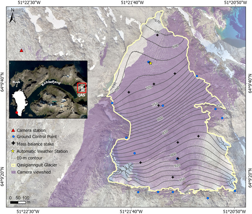
FIGURE 1. Map of Qasigiannguit glacier showing locations of time-lapse camera station and ground control points. Purple areas show the camera viewshed. The location of the automatic weather station is marked with a star. Base image is an orthophoto from a September 2020 drone survey.
The imagery used in this study is from a time-lapse camera installed at QAS (Figure 1). The camera is located on the western slope at 894 m elevation, and has taken multiple photos per day since 2014. The set-up consists of a Canon EOS 600D camera with an EF-S 18–55 mm f/3.5–5.6 IS II zoom lens and a Harbortronics Digisnap 2700 intervalometer, powered by an external battery and mounted solar panel (see Table 1 for summary of camera settings). We used images from the 2020–2021 melt seasons for mapping snowline, and referred to images taken from 2014 to 2021 to estimate timing of melt onset and total melt duration. Only camera images after the 20/08/2020 were used for snowline mapping. This was due to a shift in camera station orientation and therefore a lack of usable Ground Control Points (GCPs) prior to this date.
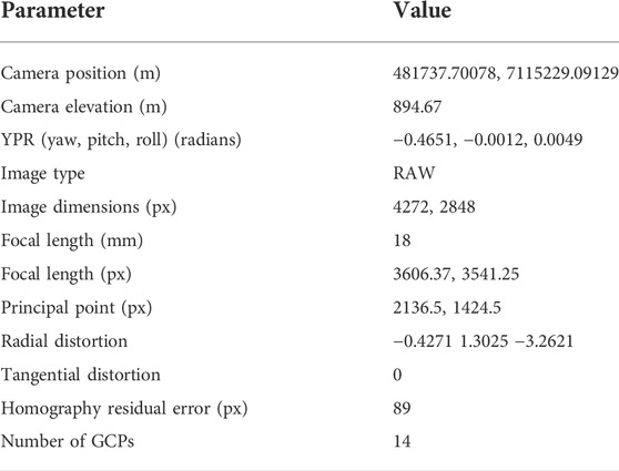
TABLE 1. Time-lapse camera settings and parameters.
A surface mass balance program has been running on the glacier as part of the Greenland Ecosystem Monitoring Programme (GEM: https://g-e-m.dk/) since 2012. This consists of a network of eleven stakes across the glacier and bi-annual visits to determine the winter and net balance. Field measurements for the 2019/2020 and 2020/2021 summer balance were carried out during field visits on 02/09/2020 and 10/09/2021. These data are submitted annually to the World Glacier Monitoring Service (WGMS: https://wgms.ch/ggcb/) and GEM (Christensen and Topp-Jørgensen, 2021) (https://g-e-m.dk/gem-publications-and-reports/gem-annual-report-cards).
In 2014, an AWS was added to the monitoring program at QAS, in collaboration with the Programme for Monitoring the Greenland Ice Sheet (PROMICE, https://promice.org/). The AWS is placed on the lower section of the glacier, close to Stake 2 at approximately 710 m elevation (Figure 1). It measures an array of parameters to calculate surface and energy balance (Abermann et al., 2019; Fausto et al., 2021). Here, we use the air temperature data to calculate Positive Degree Days (PDD), and the sonic ranger (SR50) and the pressure transducer to estimate the onset of ice melt (Hock, 2003). The sonic ranger is suspended above the surface, whilst the pressure transducer is drilled into the ice.
Time-lapse images from 2014 to 2021 were used to estimate the timing of bare ice onset and end-of-season snowline, where images were not occluded by cloud, rain or snow. Bare ice onset was here defined where bare ice was visible anywhere on the glacier within the camera viewshed. End-of-season snowline was the date of the last image before full snowfall coverage on the glacier.
Only camera images after the 20/08/2020 were used for snowline mapping. This was partly due to a shift in camera station orientation and therefore a lack of usable Ground Control Points (GCPs) prior to this date. Two approaches were adopted to classify snow-covered/bare-ice areas from the 2020/2021 images: 1) manually delineating snowline as a line feature, and 2) manually delineating bare-ice (i.e. snow-free) areas as polygon features. Snowline positions and bare ice areas were digitised manually on all cloud-free images from the 2020 (2nd September to 15th September) and 2021 (9th July to 12th September) melt seasons. Areas were delineated separately in cases where multiple bare ice areas were present in the same image.
A planar transformation projection model was used to transform the classified areas from the 2D image plane to 3D positions, as provided in PyTrx. A 5.7 cm-resolution Digital Elevation Model (DEM) was used for the georectification, which was derived from a September 2020 survey using an Ebee fixed-wing Uncrewed Aerial Vehicle (UAV). GCPs were used to optimise the projection model, as is standard practise in glacial photogrammetry studies (e.g. Messerli and Grinsted, 2015; Schwalbe and Maas, 2017), where static points on the surrounding bedrock were marked out with paint in the field prior to the drone survey. These GCPs were subsequently identified and matched between the drone survey orthophoto and the time-lapse camera images, producing an optimised pixel error of 36 pixels.
Snowline classification and mapping of snow cover and bare ice derived from terrestrial time-lapse photogrammetry are subject to two main sources of uncertainty: 1) error in the georectification process to transform coordinates between the image plane (u,v) and physical space (x,y,z); and 2) uncertainty in the manual delineation of snow and ice area estimates.
Error in the georectification process is introduced from uncertainty in the homography model generated during image registration, where image pairs are aligned to account for shifts in the camera platform. The mean pixel error in the homography model for each image pair was 86.8 pixels. An additional source of georectification error comes from the horizontal and vertical accuracy of the DEM, which creates discrepancies between positions in the image plane and the associated physical space represented by the DEM. The DEM’s horizontal accuracy (total Root Mean Square Error) is 0.074 m, with a maximum error of 0.218 m, as calculated from the difference between the surveyed GCP positions and the corresponding UAV positions and elevations. The camera model is optimised in order to account for this in the georectification process, producing a mean pixel error of 36.5 pixels.
The second main source of uncertainty is in the manual delineation of snow and ice areas from the time-lapse camera imagery, which stems from human error. Small and isolated snow/ice patches were excluded because they were too small to accurately delineate. In addition, the camera viewshed limits the visible extent of the glacier, meaning bare ice on the lower and upper steeper-slope eastern portions of QAS cannot be mapped from the oblique camera images (Figure 1). Overall, this means bare-ice areas delineated manually are underestimates. To account for this, all bare ice and snow-cover areas we report have been calculated relative to the total area of QAS visible by the camera viewshed. In addition, we delineated bare ice areas from six time-lapse camera images taken throughout 1 day (21/08/2021) at hourly intervals in the morning (03:49 to 05:48) and evening (18:49 to 20:49), in order to test the methodology’s sensitivity to the time of day the image was taken. We also tested this on a different day earlier in the melt season (29/07/2021) at hourly intervals in the morning (02:46 to 05:46) and evening (18:46 to 22:46). The findings from this sensitivity analysis are reported in Section 4.1.
Offsets between classified snowline and the UAV-derived orthophoto were noted in the high-elevation regions furthest away from the camera (Figure 2). This offset is due to shadowing and steep topography, introducing error in this region of the DEM. We calculated a positional shift of −50.84 m in the Easting (X) direction, +7.27 m in the Northing (Y) direction and +3.38 m in the vertical (Z) direction between the bare ice polygon manually delineated in PyTrx from the 02/09/2019 camera image and the snowline position on the orthophoto, taken on the same date. This offset coefficient was only applied to the classified snowlines to correct for this source of error for the dates that correspond to the mass balance stake field measurements, which are presented in Section 4.4.
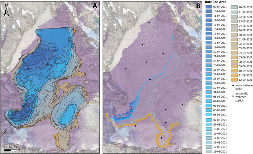
FIGURE 2. Evolution of (A) bare-ice area derived from manually-delineated polygons in PyTrx and (B) snowline derived from manually-delineated lines in PyTrx on QAS during the 2021 summer melt season. Note bare ice areas and snowlines up until 12th September 2021 are shown, which is the last date before several light snowfall events partially cover the bare ice. Melting then continues until 28th October (Figure 4). Camera viewshed is shown in purple. Locations of mass balance stakes and the AWS are shown in Panel (B).
In 2020, bare-ice patches started to form on the middle and lower portions of QAS on 10th July, based on visual inspection of the time-lapse imagery. These coalesced on 1st August and by 8th August the entire lower portion of QAS was snow-free. On 2nd September, the day of the summer mass balance measurements at QAS, 70% of QAS was bare ice (Figure 3B) and the maximum snowline elevation was 962 m above sea level (m a.s.l) (Figure 4). The end-of-season SLA (i.e. the day before the first snowfall) was on 15th September, and reached a maximum elevation of 967 m a.sl. By this date, 76% of QAS was snow-free (Figure 3B). Bare ice was visible on QAS for a total of 67 days in the 2020 melt season.
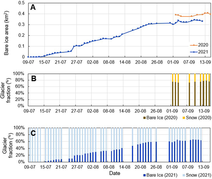
FIGURE 3. Evolution of bare-ice area during 2020 and 2021 (A) and fraction of QAS covered by bare ice and snow during the 2020 (B) and 2021 (C) summer melt seasons, derived from manually-delineated polygons in PyTrx. Bare ice and snow-cover areas have been calculated relative to the total area of QAS visible by the camera viewshed. Note in 2021 that bare ice area and bare ice/snow fractions up until 12th September 2021 are shown, which is the last date before several light snowfall events partially cover the bare ice. Melting then continues until 28th October (Figure 4).
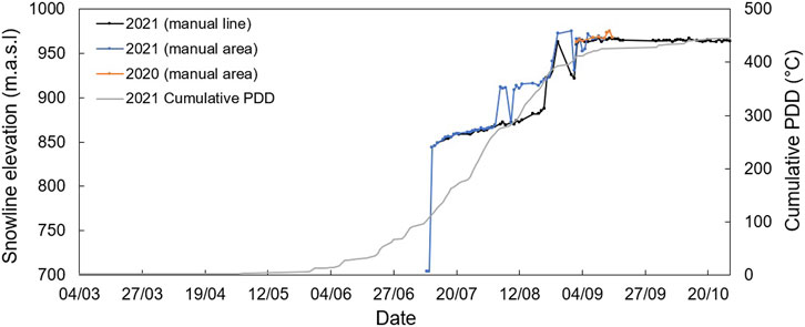
FIGURE 4. Maximum snowline elevation on QAS during the 2020 and 2021 summer melt seasons, derived from manual classification in PyTrx. Snowline positions delineated as lines are shown in black. Snowline positions (i.e. bare ice areas) delineated as polygons are shown in blue and orange. Each individual dot represent the maximum elevation of a snowline position classified from a single time-lapse camera image on one date in the melt season. The drop in maximum snowline elevation on the 9th August 2021 is due to light snowfall covering the bare ice patches on the upper portion of QAS, which subsequently melted the following day.
In 2021, a small bare-ice patch started to form on the lower portion of QAS on 9th July (covering
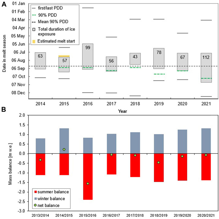
FIGURE 5. (A) Timings of onset of bare ice exposure (i.e. the date that bare ice is first visible on QAS) and total ice exposure duration (i.e. the total duration in days that bare ice is visible up until the first day of full snowfall coverage, labelled in each bar) from time-lapse camera images taken between 2014 and 2021. The first and last PDDs for each melt season are marked by horizontal black lines. The average date when 90% PDD is reached is marked as a black dashed line. In 2014, the AWS was set up after the start of the melt season so only the end of season PDD is available. In 2015, the start date of the melt season is estimated in yellow based on the average start date from camera images in other melt seasons. (B) Winter balance, summer balance and net balance from mass balance stakes on QAS. Stake locations are shown in Figure 2B.
From mid-September 2021, there were several light snowfall events which thinly covered visible bare ice and then subsequently partially melted leaving some snow patches in small surface depressions. The complexity of these ice/snow surface features made the manual delineation of bare ice extent unfeasible. These data are therefore not presented in Figure 3. However, the gross snowline position was still clearly definable (Figure 4). As a result, we could continue to map the snowline until the first snowfall on 28th October, after which no bare ice was exposed again during the season.
We observe large fluctuations in the exposure and total duration of bare ice between 2014 and 2021 on QAS, reflected in both the time-lapse images and the AWS observations (Figure 5A and Table 2). Onset of ice exposure varied between 3rd June (in 2016) and 20th July (in 2015 and 2017). The end-of-season snowline date (i.e. the last day that bare ice is visible before the first full snowfall coverage where no bare ice is exposed after this date) varied between 21st August (in 2018) and 28th October (in 2021). The season with the longest duration of ice exposure was 2021 (112 days) and the shortest duration of ice exposure (and therefore the longest duration of snow cover) was in 2018 (43 days).
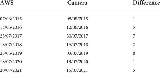
TABLE 2. Date according to the AWS mounted sonic ranger sensor and the pressure transducer that appear to indicate no snow at the AWS, compared to the date it appears to be bare ice according to the time-lapse camera imagery.
The net annual balance since 2013/2014 has largely been negative, with a mean net balance of −0.31 m w.e. (Figure 5B). The 2015/2016 period was a markedly negative net balance (−1.57 m w.e.), whilst the prior period (2014/2015) was the only positive net balance (0.22 m w.e.) observed in this study. Winter balance has an average inter-seasonal variability of 0.5 m w.e., ranging between 0.80 m w.e. (2013/2014) and 1.33 m w.e. (2014/2015). The difference between the maximum and minimum summer balances is much higher (1.31 m w.e.), largely due to the large negative summer balance of 2015/2016 (−2.403 m w.e.).
The summer balance for the 2019/2020 and 2020/2021 seasons were similar, differing by 0.007 m w.e., whilst the winter balance was 1.26 and 1.32 m w.e., respectively (Figure 5B). The net balance for both these seasons were negative for all stakes, except for the highest stake at an elevation of 943 m. The ELA was estimated to be 933 m and 934 m for 2020 and 2021, respectively.
PDD results signify the first and last PDD for each year of the study (Figure 5A) and the total PDD and date when 90% and 95% cumulative PDD is reached (Table 3). The year 2016 had the largest total PDD of 667.02°C, spanning between 17th January to 15th October. The year 2015 had the shortest PDD time range from 17th June to 15th October, whilst the year 2018 experienced the smallest total PDD (333.56°C).
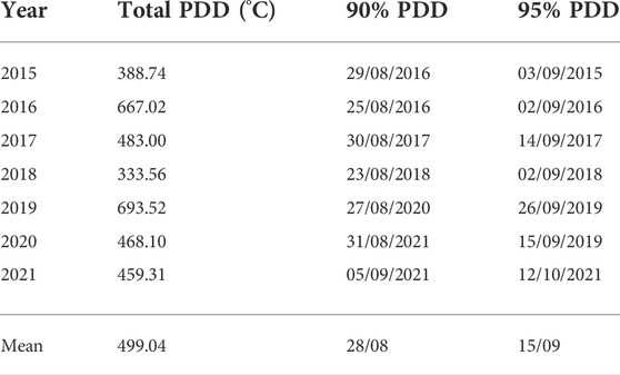
TABLE 3. Total annual PDD, and the dates in each melt season when 90% and 95% of the cumulative PDD are reached.
Comparing the more recent seasons, the onset of PDDs was earlier in 2021 than 2020 (Figure 6). High temperatures in May to mid-June resulted in rapid change in cumulative PDD during the snow melt period in 2020; continuing throughout the summer with the exception of late August. In 2021, the rate of cumulative PDD change was much less rapid in the spring. The total PDD was higher in 2020 than 2021, and was reached approximately 2 months earlier in 2020.
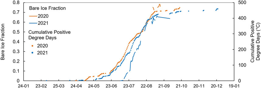
FIGURE 6. Fraction of Bare Ice versus Cumulative Positive Degree Days on QAS during 2020 and 2021.
The average total PDD per year for the study period was 499.04°C, with the average date of the year for 90% and 95% PDD being 28th August and 15th September, respectively (Table 3). Beyond 90% PDD, cumulative PDD is discontinuous, or intermittent, which results in a negligible amount of melt production.
The classification of bare ice from time-lapse imagery is highly sensitive to the time of day the image is captured. On the 2 days we investigated this sensitivity, we found the largest differences in bare ice areas were between early morning and evening. For example, at 05:48 on 21st August 2021, bare ice coverage was 0.23 km2, but at 18:49 on the same day, bare ice coverage was calculated as being only 0.01 km2 (accounting for the proportion of QAS not visible from the camera viewshed). Similarly, at 02:46 on the 29th July 2021, bare ice coverage was 0.32 km2, but at 22:46 on the same day was calculated as being only 0.04 km2. This difference arises from lower sun angles at later times of day casting shadows across the lower portion of QAS, resulting in bare ice being underestimated. For images taken within the same time of the day (i.e. morning or evening) at hourly intervals, there is a smaller difference in bare ice areas (0.2–0.32 km2 on 29th July between 02:46 and 05:46, 0.18–0.23 km2 on 21st August between 03:49 and 05:48). Overall, this sensitivity analysis demonstrates the importance of image timing and selected pixel thresholds in bare ice classification.
The exposure of bare ice according to the AWS pressure transducer and sonic ranger matches well with the date defined by the camera (Table 2). Discrepancies are on the order of a few days to a week, with the largest difference (8 days) observed for the year 2019. These discrepancies likely reflect the challenges in interpreting the pressure transducer and sonic ranger datasets, in order to accurately pick the day at which all snow has melted away, exposing the previous seasons ice surface. This data is extremely localised to the exact measurement footprint of the respective sensor. The spatial overview provided by the camera also highlights the impact itself of the presence of the AWS, which alters snow distribution around the station and can lead to a bias in the timing of the ice exposure. In addition, the locational bias in the AWS observations do not reflect glacier-wide conditions. Validation data, such as from time-lapse cameras, provide a spatial context that offer a more realistic perspective when combined. Overall, this highlight the need for validation datasets to constrain AWS observations of surface conditions, such as the timing of bare ice exposure at the AWS.
According to the shift-corrected time-lapse data, the snowline elevation was 912.90 m a.s.l. at the location along the mass balance stake transect between the upper two stakes on 02/09/2020. The estimated ELA for 2020 from the upper two stakes was estimated to be 933.00 m a.s.l. For 2021 (10/09/2021), the camera-derived snowline elevation was 918.30 m a.s.l. whilst the stake-derived ELA was 934 m a.s.l. Therefore, the elevation difference between the camera-derived snowlines and the ELA stake measurements were 20.00 m and 15.70 m for 2020 and 2021, respectively. The snowline and ELA measurements thus demonstrate good correspondence for this location on the glacier.
In the 2 years where we have overlapping data between the mass balance and the delineated time-lapse snowline, it appears that the stake mass balance data for the upper two stakes slightly overestimates the snowline elevation. However, we find that the stake ELA is much lower if we include data from all 11 mass balance stakes, with the estimated ELA being at 908.00 m a.s.l. and 880.00 m a.s.l. in 2020 and 2021, respectively.
Overall, the inter-comparison between the camera data and the stake measurements highlights the importance to adopt multi-method datasets to better understand mass balance results. The spatial data derived from the camera images enables us to interpret small differences between mass balance years; for example, due to differences in the amount of bare ice exposed to melt compared to that of snow. The AWS data provides a multitude of high-resolution time series, but its uses in identifying spatial patterns and complexities is particularly limited in mountain glacier studies. This is reflected in the comparison with the camera-derived datasets, where shadowing, localised redistribution of snow, and heterogeneous patterns of bare ice exposure are evident (Table 2 and Figures 2, 5).
Overall we find a good agreement between the number of days of visible bare ice on the glacier, the cumulative PDD, and the net surface mass balance. Both 2016 and 2019 stand out as the most negative mass balance years, with the earliest onset of PDD and greatest cumulative total PDD (Figures 5A, 6). 2017, 2018 and 2021 had very similar net balance of −0.051, −0.088, and −0.072 m w.e., respectively. They were also 3 years with low total PDD (Table 3). The duration of bare ice exposure prior to the mean 90% cumulative PDD (28th August, Table 3) is also similar in each of the aforementioned years.
Bare ice exposure is similar in 2020 and 2021, specifically prior to the mean 90% cumulative PDD (28th August, Table 3) (Figure 5A). However, this is not reflected in net balance, with a greater negative net balance of 0.142 m w.e. in 2020 (Figure 5B). Differences in net balance likely arise from a slightly higher winter balance in 2020/2021 compared to 2019/2020. Additionally, the onset of melt occurs earlier in 2020, as reflected in the cumulative PDD curves, despite the first PDD being much earlier in 2021 (Figure 6). The overall total PDD before the mean 90% cumulative PDD (28th August, Table 3) is higher in 2020 (400.56°C) than in 2021 (394.15°C)).
Despite 2021 having the longest ice exposure duration in the study (112−days, Figure 5A), it had a relatively small negative mass balance (−0.072 m w.e., Figure 5B). This is likely due to intermittent snowfall in late-autumn/early-winter, which was visible on the time-lapse images. This snowfall would have reduced the effectiveness of ice melt, and the continuity of increasing PDD would have been interrupted (Figure 6). The increase in cumulative PDD therefore plateaus and the occurrence of further PDDs becomes much more intermittent and sporadic (Table 3). As a result, the amount of energy for ice melt is low and has little impact on the resulting mass balance after this date.
The years 2016 and 2019 experienced substantial periods of exposed bare ice according to the camera data. However, 2021 experienced the longest duration of bare ice exposure yet this is not reflected in the mass balance observations as expected (Figure 5B). The main difference between these years is the timing of bare ice exposure relative to the mean 90% cumulative PDD (28th August, Table 3). In 2021, the majority days of the bare ice exposure occurred after 28th August (Figure 5A). Whereas in 2016 and 2019, a large part of the duration of bare ice exposure occurs before the mean 90% cumulative PDD.
It is suggested here that the timing of bare ice exposure relative to the mean 90% cumulative PDD (28th August, Table 3) plays a critical role in surface melting and mass balance, with large negative mass balance records from 2016 to 2019 linked to long periods of bare ice exposure prior to the 28th August. This is because the date at which bare ice is exposed on the glacier depends on the amount of energy available to melt the winter snow pack as well as the thickness of the snowpack.
The importance of the timing of bare ice exposure is further reflected in the overall total PDD (as described earlier in Section 4.4). Prior to the mean 90% cumulative PDD (28th August, Table 3), the bare ice fraction is higher during August for 2020 compared to 2021. This is reflected in differences in total PDD for 2020 and 2021, with 2020 having a higher total (400.56°C) than 2021 (394.15°C), despite 2021 experiencing longer bare ice exposure. Therefore, it could be argued that the larger bare ice surface exposed in 2020 prior to the mean 90% cumulative PDD plays a greater role in ice melt than the longer bare ice exposure experienced in 2021.
Opportunities to extend this work include expanding the time-series of snowline and bare ice evolution to include data from 2014 to 2020. The time-lapse camera data requires refining the projection model with new GCPs to ensure precise georectification of bare ice areas. A possibility for addressing mis-classifications from the workflow would be to include a shadow modelling module using the DEM in order to remove shadowing (Schwalbe and Maas, 2017). Shadows could then be automatically removed before classifying bare ice areas.
The snowline positions and bare ice areas presented here could serve as a useful comparison to satellite-derived snowlines. Each approach to snowline mapping offers its own advantages and limitations. While terrestrial time-lapse imagery provides a high temporal and spatial resolution source of ground truth snow cover data, it is restricted to a small geographic area and a limited number of sites (Härer et al., 2016). Satellite imagery offers the advantage of a larger spatial footprint and longer-term return period to monitor catchments over an extended period, albeit at a medium resolution (i.e. metres to tens of metres). Therefore, a combined approach using both of these image sources would be beneficial for assessing snowline evolution on local peripheral glaciers around whole regions of the ice sheet.
One of the main findings from this study is the importance of the spatial distribution of snow and bare ice across the glacier. This is crucial for mountain glaciers where topography plays a huge role in the heterogeneous melting of snow. In particular, traditional snowline studies assume an elevation of snowline, and thus also energy input for melting. However, this is not observed at QAS where persistent snow patches exist at low elevations and ice is exposed at higher elevations on the glacier at the start of the melt season. This has far reaching implications for mass balance modelling efforts, where it has been demonstrated that spatial variability in glacier surface characteristics is linked to different melt factors and energy required to melt snow and ice. A snowline can give a rough indication, but the findings from QAS reveal that the situation is far more complex. Accurate estimates of mass loss from glaciarised mountain catchments can only be achieved with a deeper knowledge of the spatial evolution of the snow-to-bare-ice ratio throughout the melt season.
Using manual snowline extraction from terrestrial time-lapse photogrammetry, we produced a time-series of maximum snowline elevation and the extents of snow and bare ice through the 2020 and 2021 melt seasons. Additionally, we compared this data to a comprehensive 8 years record of mass balance and AWS data from QAS glacier. Overall we find a good agreement between the snowline elevation from the time-lapse data and the stake mass balance data. The corresponding snowline value from the day of summer mass balance measurements in 2020 and 2021 show an overall discrepancy in elevation of 20 m and 15.7 m, respectively, compared to the forecast ELA compiled from measured mass balance stake data. Snowline classification accuracy is sensitive to image cloud cover and illumination, spectral similarities in snow and ice facies, and the diffuse nature of the snow-ice boundary. Nevertheless, we were able to produce a high resolution spatio-temporal time series of the snow and bare ice area evolution over the entire glacier.
This study highlights some of the challenges when interpreting mass balance data, especially the variations between years. It demonstrates the importance of having a spatial overview of the surface conditions at the glacier, especially mountain glaciers with varying topography. In particular, this refers to the timing of bare ice exposure as defined by spatially-limited single point data at the AWS compared to that of the spatial context of time-lapse images. The date of ice exposure at QAS was detected much earlier in the camera data than at the AWS. This highlights the importance of AWS placement, especially in mountain glacier settings, and the challenges associated with extrapolating AWS across an entire glacier. An important finding is that the date of ice exposure timing in relation to the mean 90% cumulative PDD is a key component for ice melt and mass balance. Ice exposure after this threshold date appears to have little impact of the resulting mass balance, compared to the amount of days prior to the 90% cumulative PDD. This is clearly evident in the 2021 season, which has the longest ice exposure duration yet a relatively small negative mass balance due to the majority of the bare ice exposure occurring after this threshold date. Overall, this is crucial for future modelling efforts on peripheral mountains glaciers such as QAS, as the complexity of surface conditions and timings of bare ice exposure are currently not represented and yet have a large implications for mass balance.
The raw AWS data are available through both the PROMICE (https://dataverse.geus.dk/dataset.xhtml?persistentId=doi:10.22008/FK2/8SS7EW) and GEM (https://data.g-e-m.dk/) databases. The original time-lapse imagery is available on request. A working example of the time-lapse image processing workflow from Qasigiannguit Glacier is available with https://github.com/PennyHow/PyTrx/releases/tag/pytrx1.2.4.
AM designed the initial study and lead the paper. JAr derived snowlines from the time-lapse camera imagery and produced the associated figures. KL was responsible for the processing of the mass balance and climate data. PH developed the Python-based toolbox PyTrx and assisted with all PyTrx-related processing. All authors were responsible for writing and editing the main body of the manuscript.
AM, KL, PH, and JAb were funded to different extents by the Greenland Research Council (NIS), GlacioBasis Nuuk under the Greenland Ecosystem Monitoring Programme (GEM), and through the Danish Ministry of Climate, Energy and Utilities via The Programme for Monitoring of the Greenland Ice Sheet (PROMICE) and the Greenland Climate Network (GC-Net). PH had additional funding under the ESA Living Planet Fellowship (grant number 4000136382/21/I-DT-lr). JAr was supported by the IAPETUS Natural Environment Research Council (NERC) Doctoral Training Partnership (grant number NE/L002590/1), which funded a PhD placement to Asiaq Greenland Survey.
We would like to thank the two reviewers for providing constructive comments which led to improvement of this paper and the editor for handling the manuscript.
The authors declare that the research was conducted in the absence of any commercial or financial relationships that could be construed as a potential conflict of interest.
All claims expressed in this article are solely those of the authors and do not necessarily represent those of their affiliated organizations, or those of the publisher, the editors and the reviewers. Any product that may be evaluated in this article, or claim that may be made by its manufacturer, is not guaranteed or endorsed by the publisher.
[Dataset] Abermann, J., As, D. V., Petersen, D., and Nauta, M. (2014). A new glacier monitoring site in West Greenland. (Accessed 11 22, 2021).
Abermann, J., As, D. V., Wacker, S., Langley, K., Machguth, H., and Fausto, R. S. (2019). Strong contrast in mass and energy balance between a coastal mountain glacier and the Greenland ice sheet. J. Glaciol. 65, 263–269. doi:10.1017/jog.2019.4
Andreassen, L., Moholdt, G., Kääb, A., Messerli, A., Nagy, T., and Winsvold, S. H. (2021). Monitoring glaciers in mainland Norway and Svalbard using SentinelNVE Rapport nr. 3/2021. (Norwegian Water Resources and Energy Directorate).
Banwell, A., Willis, I., Arnold, N., Messerli, A., Rye, C., Tedesco, M., et al. (2012). Calibration and evaluation of a high-resolution surface mass-balance model for Paakitsoq, West Greenland. J. Glaciol. 58, 1047–1062. doi:10.3189/2012JoG12J034
Barandun, M., Huss, M., Usubaliev, R., Azisov, E., Berthier, E., Kääb, A., et al. (2018). Multi-decadal mass balance series of three Kyrgyz glaciers inferred from modelling constrained with repeated snow line observations. Cryosphere 12, 1899–1919. doi:10.5194/tc-12-1899-2018
Bjørk, A. A., Aagaard, S., Lütt, A., Khan, S. A., Box, J. E., Kjeldsen, K. K., et al. (2018). Changes in Greenland’s peripheral glaciers linked to the North Atlantic Oscillation. Nat. Clim. Change 8, 48–52. doi:10.1038/s41558-017-0029-1
Bolch, T., Sørensen, L. S., Simonsen, S. B., Mölg, N., Machguth, H., Rastner, P., et al. (2013). Mass loss of Greenland’s glaciers and ice caps 2003–2008 revealed from ICESat laser altimetry data. Geophys. Res. Lett. 40, 875–881. doi:10.1002/grl.50270
Christensen, M. A., and Topp-Jørgensen, E. (2021). Greenland ecosystem monitoring annual report cards 2020. Aarhus, Jutland, Denmark: DCE—Danish Centre for Environment and Energy, Aarhus University, 44.
Cogley, J., Hock, R., Rasmussen, L., Arendt, A., Bauder, A., Braithwaite, R., et al. (2011). Glossary of glacier mass balance and related terms. doi:10.5167/uzh-53475
Colgan, W., Rajaram, H., Anderson, R., Steffen, K., Phillips, T., Joughin, I., et al. (2011). The annual glaciohydrology cycle in the ablation zone of the Greenland ice sheet: Part 1. Hydrology model. J. Glaciol. 57, 697–709. doi:10.3189/002214311797409668
Dozier, J. (1989). Spectral signature of alpine snow cover from the Landsat Thematic Mapper. Remote Sens. Environ. 28, 9–22. doi:10.1016/0034-4257(89)90101-6
Fausto, R. S., Andersen, S. B., Ahlstrøm, A. P., van As, D., Box, J. E., Binder, D., et al. (2018). The Greenland ice sheet – snowline elevations at the end of the melt seasons from 2000 to 2017. GEUS Bull. Rev. Surv. Activities 41, 71–74. doi:10.34194/geusb.v41.4346
Fausto, R. S., van As, D., Mankoff, K. D., Vandecrux, B., Citterio, M., Ahlstrøm, A. P., et al. (2021). Programme for monitoring of the Greenland ice sheet (PROMICE) automatic weather station data. Earth Syst. Sci. Data 13, 3819–3845.
Härer, S., Bernhardt, M., and Schulz, K. (2016). Practise – photo rectification and classification software (v.2.1). Geosci. Model. Dev. 9, 307–321. doi:10.5194/gmd-9-307-2016
Hugonnet, R., McNabb, R., Berthier, E., Menounos, B., Nuth, C., Girod, L., et al. (2021). Accelerated global glacier mass loss in the early twenty-first century. Nature 592, 726–731. doi:10.1038/s41586-021-03436-z
Huss, M., Sold, L., Hoelzle, M., Stokvis, M., Salzmann, N., Farinotti, D., et al. (2013). Towards remote monitoring of sub-seasonal glacier mass balance. Ann. Glaciol. 54, 75–83. doi:10.3189/2013AoG63A427
[Dataset] Hynek, B., Weyss, G., Binder, D., Schöner, W., Abermann, J., and Citterio, M. (2014). Mass balance of freya glacier. Greenland since 2007/2008. doi:10.1594/PANGAEA.831035
Machguth, H., Thomsen, H. H., Weidick, A., Ahlstrøm, A. P., Abermann, J., Andersen, M. L., et al. (2016). Greenland surface mass-balance observations from the ice-sheet ablation area and local glaciers. J. Glaciol. 62, 861–887. doi:10.1017/jog.2016.75
Mernild, S. H., Liston, G. E., Hasholt, B., and Knudsen, N. T. (2006). Snow distribution and melt modeling for Mittivakkat Glacier, ammassalik island, southeast Greenland. J. Hydrometeorol. 7, 808–824. doi:10.1175/JHM522.1
Messerli, A., and Grinsted, A. (2015). Image georectification and feature tracking toolbox: ImGRAFT. Geoscientific Instrum. Methods Data Syst. 4, 23–34. doi:10.5194/gi-4-23-2015
Racoviteanu, A. E., Rittger, K., and Armstrong, R. (2016). An automated approach for estimating snowline altitudes in the Karakoram and Eastern Himalaya from remote sensing. Front. Earth Sci. 7. doi:10.3389/feart.2019.00220
Rastner, P., Prinz, R., Notarnicola, C., Nicholson, L., Sailer, R., Schwaizer, G., et al. (2019). On the automated mapping of snow cover on glaciers and calculation of snow line altitudes from multi-temporal Landsat data. Remote Sens. 11, 1410.
Ryan, J. C., Smith, L. C., Cooley, S. W., Cooper, M. G., Pitcher, L. H., and Hubbard, A. (2019). Greenland ice sheet surface melt amplified by snowline migration and bare ice exposure. Sci. Adv. 5. doi:10.1126/sciadv.aav3738
Schwalbe, E., and Maas, H.-G. (2017). The determination of high-resolution spatio-temporal glacier motion fields from time-lapse sequences. Earth Surf. Dyn. 5, 861–879. doi:10.5194/esurf-5-861-2017
Keywords: time-lapse, mass balance, Greenland, snow, glacier
Citation: Messerli A, Arthur J, Langley K, How P and Abermann J (2022) Snow cover evolution at Qasigiannguit Glacier, southwest Greenland: A comparison of time-lapse imagery and mass balance data. Front. Earth Sci. 10:970026. doi: 10.3389/feart.2022.970026
Received: 15 June 2022; Accepted: 25 July 2022;
Published: 24 August 2022.
Edited by:
Bartłomiej Luks, Polish Academy of Sciences, PolandReviewed by:
Niccolo Dematteis, National Research Council (CNR), ItalyCopyright © 2022 Messerli, Arthur, Langley, How and Abermann. This is an open-access article distributed under the terms of the Creative Commons Attribution License (CC BY). The use, distribution or reproduction in other forums is permitted, provided the original author(s) and the copyright owner(s) are credited and that the original publication in this journal is cited, in accordance with accepted academic practice. No use, distribution or reproduction is permitted which does not comply with these terms.
*Correspondence: Alexandra Messerli, YW1lQGFzaWFxLmds
Disclaimer: All claims expressed in this article are solely those of the authors and do not necessarily represent those of their affiliated organizations, or those of the publisher, the editors and the reviewers. Any product that may be evaluated in this article or claim that may be made by its manufacturer is not guaranteed or endorsed by the publisher.
Research integrity at Frontiers
Learn more about the work of our research integrity team to safeguard the quality of each article we publish.