 Pasquale De Gori
 Francesco Pio Lucente
 Aladino Govoni
 Lucia Margheriti
 Claudio Chiarabba
95% of researchers rate our articles as excellent or good
Learn more about the work of our research integrity team to safeguard the quality of each article we publish.
Find out more
ORIGINAL RESEARCH article
Front. Earth Sci. , 10 November 2022
Sec. Solid Earth Geophysics
Volume 10 - 2022 | https://doi.org/10.3389/feart.2022.968187
This article is part of the Research Topic Earthquake Swarms and Complex Seismic Sequences in Tectonic and Volcanic Areas View all 6 articles
Seismic swarms frequently occur along continental fault systems and their relation with large earthquakes is often contradictory. Such a case is documented in the Pollino mountain range of southern Italy, a decoupling zone where the belt-normal stretching drastically rotates accommodating the differential SE-retreat of the Ionian slab. The paucity of historical large earthquakes has led to hypothesize the presence of a seismic gap. A long-lasting seismic swarm that climaxed with a ML = 5.2 earthquake in October 2012 was therefore thought as a possible signal of an impending large earthquake filling the gap. Seismicity data collected during a 4-years long monitoring are a powerful microscope to look through the seismic swarm. In this study, we present accurate relocations for 2385 earthquakes and high-resolution Vp and Vp/Vs models of the fault system. Seismicity occurred on two separate normal faults that were formerly part of a thrusts and back-thrusts system, originally formed as a pop-up at restraining bends of the Pollino fault, a wrench fault system that inverted the original left lateral sense of slip accommodating a differential motion induced by the southward retreat of the Ionian slab.
Seismic swarms in tectonically active regions often consist in recrudescent bursts of seismicity that liberate in a complex and disordered pattern only a small fraction of the strain energy accumulated by tectonic stresses (Hardebeck et al., 2008; Wu et al., 2014). Although their meaning in terms of short term hazard and their precursory aspect are always enigmatic, they allow the investigation of fault geometry, rheology and more in general of the earthquake processes including the relation between fluid pressure, aseismic deformation and seismicity (Holtkamp and Brudzinski, 2014; Zhang et al. 2019; De Barros et al. 2020; Ross et al 2020; Bachura et al. 2021).
During 2010–2015, intense seismic swarms developed in the area between the Calabrian Arc and the Apennines (Govoni et al., 2013), at the edge of the Ionian subduction (Totaro et al., 2014; Orecchio et al., 2015; Chiarabba et al., 2016; Palano et al., 2017). This area has for long times retained a major seismic gap of peninsular Italy (Tertulliani and Cucci, 2014, and references therein). The lack of large historical events on a 100 km long section of an apparently continuous normal faulting system, edged by faults that ruptured many times, concurred to frame such a hypothesis, after the pioneering intuition of Omori (1894). Therefore, the seismic unrest has been monitored with accuracy and became a great opportunity to investigate the gap hypothesis.
Active faults at the Calabria-Lucania border (Figure 1) comprise both NW-SE trending SW and N-S striking E dipping normal fault sets (Brozzetti et al., 2017). Although with some discordance on fault geometry, paleoseismic studies found evidences for slip occurred in the past ten thousand years and consistent with M>6 earthquakes (Cinti et al., 1997, 2002; Michetti et al., 1997) advocating for the presence of major seismogenic faults in this gap area. Framing the gap hypothesis, seismic catalogs did not report large earthquakes in historical time in the Pollino area, while they are present just north and south of the area (Tertulliani and Cucci 2014; Rovida et al., 2016). A few earthquakes with magnitudes probably less than 6 are documented, including the MW = 5.6 “Mercure” event in 1998 (Brozzetti et al., 2009). Although historical earthquakes are lacking, the seismic hazard map reports a 10% chance of exceed 0.225 g in the next 50 years (Gruppo di Lavoro, 2004) and a recent work stressed how a mixed seismic/aseismic strain release pattern could favor a longer recurrence time for large magnitude earthquakes (Cheloni et al., 2017).
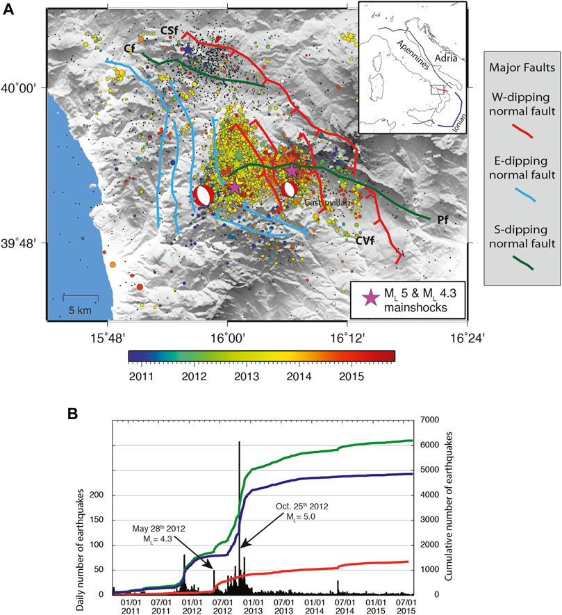
FIGURE 1. (A) Map of the 2010–2015 seismic sequence/swarm from ISIDe Working Group (2016), https://doi.org/10.13127/ISIDE. The size of the epicenters is proportional to the magnitude. Stars are the largest events (ML > 3.5), including the two mainshocks. Earthquakes are color-coded by time of occurrence according to the scale on bottom. The red beach balls indicate the 28 May 2012, ML = 4.3 (on the west) and the 25 October 2012, ML = 5.2 (on the east) mainshocks, respectively (solutions are taken from http://cnt.rm.ingv.it/tdmt.html; Scognamiglio et al., 2009). Major active faults, in the Calabria-Basilicata border region (modified after Brozzetti et al., 2017) are also drawn on the map: Castelluccio fault (Cf); Castello Seluci-Viggianello-Piano di Pollino-Castrovillari fault set (CSf); Castrovillari fault (CVf); Pollino Line (Pf). (B) Temporal evolution of the sequence/swarm: black histogram defines the daily number of events, the green line is the cumulative number of events in the whole region, the blue line and the red line are the cumulative number of events for the western and eastern cluster, respectively (modified after Pastori et al., 2021).
Previous analyses of the 2010–2015 swarm revealed that seismicity occurred along two main NNW-trending independent clusters, while the fault geometry has been interpreted differently (Passarelli et al., 2015; Pastori et al., 2021; Napolitano et al., 2020 and, 2021; Cirillo et al., 2022). Moreover, the relation between the swarm seismicity and the main faults observed at the surface remains ambiguous, as well as the general mechanism of deformation in the area. Palano et al. (2017) described a drastic change in kinematics across the range, while also the crustal structure north and south of the Pollino is very different (Bigi et al., 1992). Such complexity lands many aspects still unsolved, from the intrinsic validity of the gap hypothesis to the real meaning of the seismic swarms.
In this work, we addressed these points by accurately relocating earthquakes and defining fault structure and crustal physical state at depth with seismic tomography. Vp and Vp/Vs anomalies are used to infer insight on the seismogenic process trying to reveal the role of fluids in the faulting process. We discuss velocity anomalies taking into account the geometry of the fault system suggested by our hypocentral locations to look at seismogenesis and at specific behavior of the faults and the nature of the swarm.
The subduction of the Ionian oceanic plate beneath the Calabrian Arc is the main engine in the central Mediterranean area, along the tectonic boundary between the slowly converging Africa and Eurasia plates (e.g., Faccenna et al., 2001; Lucente et al., 2006). Slab geometry is well-documented by several seismological studies (Chiarabba et al., 2008; Giacomuzzi et al., 2012, and references therein), and the lithospheric structure of the area has been the object of different multidisciplinary studies (e.g., Di Stefano et al., 2009; Piana Agostinetti and Amato, 2009; Piana Agostinetti et al., 2009; Totaro et al., 2014; Orecchio et al., 2015).
The general image that comes from so many studies is that of a subduction panel that became progressively narrower as the retreat proceeded (Lucente et al., 2006, and references therein). Since the Late Miocene, the slab experienced rapid rollback, at a rate of 5–6 cm/yr, which was by far higher than the convergence between Africa and Europa (Faccenna et al., 2004). During the late Pleistocene, rollback and subduction have drastically slowed and at present the threnchward motion of the Calabrian arc is of about 1–3 mm/yr (D’Agostino and Selvaggi, 2004; Palano et al., 2017).
The slab retreat is coupled with extension on a continuous belt that follows the Southern Apennines ridge and extends in the Pollino region with a general decrease to the south (D’Agostino et al., 2011). Such evidence indeed reveals that the Pollino region is accumulating tectonic strain on a complex system of normal active faults (Brozzetti, 2011). More recently, Palano et al. (2017) reported a rotation of GPS velocity around the Pollino fault, evidencing a first order change between the Apennines and the Calabrian regions. The Plio-Pleistocene evolution in this zone, at the edge of the retreating Ionian slab, has been controlled by slip on a main 110° trending strike slip shear zone (Palano et al., 2017) which continues in the Ionian off-shore (Ferranti et al., 2014). Since the Middle Pleistocene, the kinematics of the shear zone switched to extensional (Schiattarella, 1998).
During past decades, a significant sequence of earthquakes followed a Mw 5.6 occurred in 1998, to the north of the Pollino area, in a region of low instrumental and moderate historical seismicity (Brozzetti et al., 2009). Seismicity was related to the Mercure fault, a normal dip-slip fault, SSW-ward dipping, whose seismogenic potential is estimated by Brozzetti et al. (2009) to be significantly larger than the 1998 earthquake (M 6.3). This implies that the Mercure 1998 earthquake would have only activated a small portion of the fault plane, turning on a warning light on the seismic hazard of both the Mercure basin and the neighboring areas.
Looking inside the Italian Seismological Instrumental and Parametric Data-Base https://doi.org/10.13127/ISIDE we observe that after a multi-years long silence, seismic activity resurged in 2010, with a series of small earthquakes (ML < 3.0). Between 2010 and early 2012, the earthquake rate has been variable (Figure 1B), with magnitudes not exceeding ML = 3.6. On 28 May 2012, a shallow ML = 4.3 event struck, about 5 km east of the previous cluster of seismicity (Figure 1A), followed by a sequence of aftershocks around it, which lasted until early August. Then, seismicity resumed to the previously activated area, with several earthquakes of magnitude larger than 3, culminating with a ML = 5.2 earthquake on 25 October 2012 (Figure 1A). The seismicity rate remained high for some months, but magnitudes did not exceed ML = 3.7. At the beginning of 2013, the seismic activity started to decrease (Figure 1B), remaining relatively low until June 2014, when a magnitude ML = 4 earthquake occurred in the eastern cluster, giving rise to a sudden increase of the seismic rate in the surrounding area (Figure 1B). Seismicity rate keeps decreasing during 2015, although remaining above the background seismicity threshold (Figure 1B).
On a map view, earthquakes, located by the Italian Seismic Bulletin and distributed in ISIDe, 2016, delineate two main clusters around the two major shocks (ML = 4.3 and ML = 5.2). Hypocenters concentrated at depths between 5 and 10 km during the entire swarm. The fault plane solutions identified by the Time Domain Moment Tensor (TDMT; http://terremoti.ingv.it/tdmt?timezone=UTC; Scognamiglio et al., 2009) for the two major events are consistent with normal faults trending ∼N25W and dipping at about 45°. On the whole, focal mechanisms are coherent with NE-SW extension (Totaro et al., 2013; 2015), moreover for events of the seismic sequence (2011–2013) Napolitano et al. (2021) shows that some of the shallowest events have a strike-slip kinematics while deeper events show an overall normal fault kinematics.
Geodetic data show a transient slip that started about 3–4 months before the ML = 5.2 and lasted almost 1 year, revealing that a significant fraction of the overall deformation is released aseismically (Cheloni et al., 2017). The transient slip correlates with the seismic rate increase (Figure 1B) consistent with seismological analyses (Passarelli et al., 2015).
A combined dataset of seismic waveforms recorded by both permanent and temporary stations (Figure 2) has been analyzed to provide high quality P and S-wave arrivals and 1D earthquake locations (Pastori et al., 2021); the temporary stations used are described in detail in a INGV Technical report (Margheriti et al., 2013). For tomographic inversion, we selected a subset of this dataset following these selection criteria: rms < 0.5 s, azimuthal gap < 220°, location errors < 1 km, a minimum of 7 P and 3 S readings, epicentral distance for the nearest station within 12 km. A total of 2385 seismic events, recorded at 27 stations (7 of which were installed soon after the occurrence of the Mw 5.2 event), provided a final number of 30,197 and 20,464 for P and S arrival times, respectively.
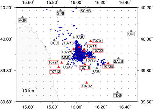
FIGURE 2. Spatial distribution of earthquakes and stations used for the tomographic inversion (in red temporary stations deployed to monitor the seismic swarms of 2011–2014). The tomographic grid is defined by nodes spaced 4 km in horizontal directions (see crosses) and 3 km along depth. The starting velocity values assigned to each node are taken by the minimum-1D velocity model of Pastori et al. (2021).
We use this dataset to compute high resolution velocity models and 3D earthquake locations by using the linearized, iterative, damped least squares inversion method Simulps14q (Haslinger, 1998). At each iteration step, earthquake locations are performed by using the singular value decomposition approach and the Vp and Vp/Vs model are updated by a damped least square inversion carried out after performing the algebraic separations between location and model partial derivatives (Haslinger, 1998, and references therein).
We used this data to solve for a 3-D grid of nodes spaced every 5 and 3 km in the horizontal and vertical directions, respectively. Starting Vp and Vp/Vs models are derived from Pastori et al. (2021). The inversion run achieved a 57% variance reduction and a final rms of 0.16 s after 9 iterations.
The reliability of the Vp and Vp/Vs tomographic models has been assessed by the analysis of resolution and covariance matrices and by running synthetic checkerboard tests. We compute the spread function (SF) as defined by Michelini and McEvilly (1991) to quantify the compactness of each averaging vector. A perfectly resolved node is characterized by an averaging vector with the diagonal element of resolution matrix equal to 1 and null off diagonal elements. In real cases, the resolution of the diagonal element is smaller than 1 and the off diagonal elements are positive values, therefore representing the volumetric estimation of the parameter. The SF accounts for all the elements of the averaging vector, quantifying the contribution of the off-diagonal elements by weighting the geometrical distance from the analyzed parameter. A compact averaging vector, i.e., a well-resolved parameter, is characterized by a small value of SF. This value increases logarithmically as long as the resolution decreases.
Since resolution is strongly dependent on the ray sampling of each node, we use the method of Toomey and Foulger (1989) for the determination of the adequate SF threshold below which the resolution is satisfactory. We analyzed how SF values relate to the derivative weighted sum (DWS), that is, an estimate of the ray sampling around each node. Points on a two-dimensional plot created by reporting SF versus the DWS of all the nodes of the model, describe a L-shaped trend with SF and DWS inversely related. The kink of L-shaped trend represents the SF value that ensures well-resolved nodes and negligible smearing (Toomey and Foulger, 1989). The tomographic inversion carried out for this study leads to plots of Figure 3, from which we infer that the SF limit is 2 for Vp and Vp/Vs models. The analysis of the covariance matrix indicates furtherly that nodes with SF ≤ 2 are characterized by formal error within the 10% of the computed velocity anomalies.
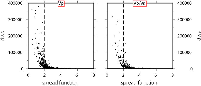
FIGURE 3. Two-dimensional plots of the Derivative weight sum (DWS) versus the Spread Function (SF) for Vp and Vp/Vs parameters. In each plot, the dashed vertical line indicates SF = 3. This value represents the kink of the L-shaped trend that represents the upper threshold of SF that ensures a good resolution and negligible smearing effects (Toomey and Foulger, 1989).
In order to examine the robustness of the retrieved tomographic anomalies we also performed a checkerboard sensitivity test. The checkerboard model was constructed by adding a 5% anomaly to the starting Vp and Vp/Vs model, therefore preserving the original grid spacing (5 × 5 × 3). Synthetic traveltimes were computed by forward calculation through the synthetic model and a Gaussian noise of zero mean and a standard deviation of 0.12 s for P- and 0.23 s for S-wave data was added to the synthetic traveltimes to simulate a real dataset. The noisy traveltimes were then inverted as in the real case starting from the same 1-D model used for the real inversion. The spatial distribution of recovered anomalies, in addition to the analysis of the SF, suggests that the threshold SF=2.0 enclose all the parts of the model characterized by good resolution and high reliability.
P-wave velocities in the upper crust are mostly influenced by lithology (Chiarabba et al., 2005). Vp ranging between 5.0 and 6.0 km/s are observed in Southern Apennines for the Mesozoic carbonates; basin filling sediments and syn-orogenic sedimentary and flysch have P-wave velocities ranging between 2.0 and 3.0, and 3.4–4 km/s respectively, whereas basement formations have the highest P-wave velocity of the sedimentary pile, with values of about 6.3 and 6.7 km/s (Improta et al., 2000 and references therein). In the area, the pre-Miocene bedrock is made of Liguridi-Sicilidi units, forming the allochthon thrust wedge (Ferranti et al., 2014). While P-wave velocity are mostly influenced by the variation of lithology in the upper crust, the Vp/Vs is more sensible to the different level of cracking in the rocks, pore aspect ratio and fluid pressure and type (Nur et al., 1972; Wang and Nur, 1989; Zhao and Negishi, 1998; Chiarabba et al., 2009). It is commonly accepted that Vp/Vs decrease from the shallow to the middle the crust as response to the increase of lithostatic pressure (i.e., Thurber and Atre, 1993). However, in uppermost crust at seimogenic depths, Vp/Vs ratio is useful in discriminating zones saturated with fluids (Nur, 1972), due to the fact that the content and the physical state of fluids affect differently the P- and S-wave velocities. In particular an increase of pore pressure forces cracks to remain open, leading to a sensible reduction of S wave velocity and to an increase Vp/Vs (Ito et al. 1979). Many recent examples show that in the upper crust high values of Vp/Vs are strongly related to fluid contents. Tomographic investigations of Apenninic normal fault systems show the presence of high Vp/Vs volumes at the base of seismogenic layer depth (8–10 km) interpreted as compartments of pressurized fluids (Chiarabba et al., 2020). In the crustal volumes surrounding the 2009 L’Aquila seismic event, time variations of Vp/Vs are found in the footwall and hanging wall of the causative fault, tracing the fluid involvement in the preparatory phase of the main event (Lucente et al, 2010).
Figure 4 shows the velocity results in the inverted volume, at 3 and 6 km depth layers, i.e., where most of the seismicity is concentrated, including the two main shocks. The surface traces of active faults are shown as colored line segments on the tomographic maps (as in Figure 1). The corresponding results of the checkerboard test are also shown on the right of each tomogram. In this 3–6 km depth range, P-wave velocity varies from about 4.5 to 7.0 km/s at 6 km depth, while Vp/Vs values vary from about 1.7 to more than 1.9.
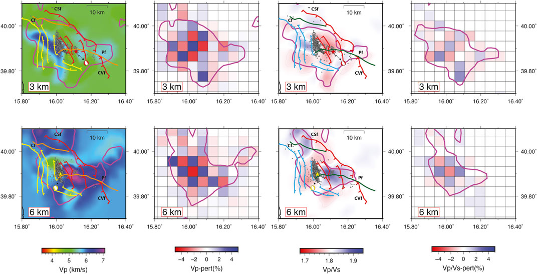
FIGURE 4. P-wave velocity (on the left) and Vp/Vs models (on the right) at the most significant depths, 3- (on top) and 6 km (on bottom), respectively. Vp and Vp/Vs values are color coded according to the color scales at the bottoms; the purple contour line represents the well resolved area in each layer. Hypocenters of the relocated events are reported in the respective layers as gray dots. The two major earthquakes are represented by red- (28 May 2012, ML = 4.3) and yellow stars (25 October 2012, ML = 5), respectively, together with their focal solution (http://cnt.rm.ingv.it/tdmt.html; Scognamiglio et al., 2009). Major active faults, as for Figure 1, are also reported on each layer, as colored line segments (on the Vp tomograms only, colors of the fault traces have been modified with respect to Figure 1, to make them more visible). For each layer (both Vp and Vp/Vs models), the corresponding results of the checkerboard test are shown on the right of each tomogram.
At 3 km depth, the shallower hypocenters are clustered at the eastern border of a relatively high velocity region (6.0 km/s), NNW-elongated, which extends further south. The 28 May 2012 ML = 4.3 event (red star in Figure 4, both Vp and Vp/Vs tomograms) struck east of the bulk of the seismicity, in a lower velocity area (5.5 km/s). The distribution of the Vp/Vs values at this depth shows a prevalence of relatively low values with few spots of relatively high values at the western border of the alignment of the hypocenters, and at the SE margin of the resolved volume. The bulk of seismicity, NNW-elongated, extends along the edge between volumes of different Vp/Vs., while the ML = 4.3 event (red star in Figure 4) struck in an area of relatively low Vp/Vs.
At 6 km depth most of the seismicity, which still shows a NNW-elongated pattern, is edged to the west and the north by a relatively low velocity region (about 5.5 km/s), and to the east and the south by a high velocity area. At the border between these low and high velocity anomalies originated the ML = 5.2 earthquake on 25 October 2012 (yellow star in Figure 4, both Vp and Vp/Vs tomograms). Highest Vp values at this depth (up to 7.0 km/s) are found east of the main alignment of earthquakes, in a region where few hypocenters are located, in correspondence to the locus where the ML = 4.3 event developed at shallower depth (red stars in Figure 4). The pattern of the Vp/Vs in the layer at 6 km depth is simpler than in the above layer. A main region of relatively high Vp/Vs is located in the central part of the layer, roughly corresponding to the highest Vp volume at this depth (from the comparison between Vp and Vp/Vs tomograms in Figure 4). Relatively high Vp/Vs values are also found in the NW part of the layer, while a broad region of relatively low Vp/Vs values is found in the western part of the layer, extending further north. The main cluster of earthquakes, containing the hypocenter of the ML = 5.2 earthquake (yellow star in Figure 4), elongates along the border between the two main areas of relatively high (to the east) and low (to the west) Vp/Vs., while the little cluster on the east, roughly in correspondence to the ML = 4.3 event in the above layer (red star in Figure 4), is located within the highest Vp/Vs volume.
The tomographic images show that the seismicity mainly develops at the edges of crustal volumes with different properties, in terms of both Vp and Vp/Vs However, it is noticeable that going from one layer to the other (from 3 to 6 km depth), the location of the low and high Vp and Vp/Vs anomalies switches with respect to the cluster of seismicity (i.e., where at 3 km depth a low anomaly is found, at 6 there is a high anomaly). Furthermore, we observe that the seismicity is almost entirely included within the projection at depth of opposing-dipping faults traces.
The values of the P-wave seismic velocity, the switch of Vp and Vp/Vs anomalies with depth, and the location of the seismicity at the edges between opposite anomalies suggests, respectively, that the seismicity occurs within a carbonate unit, that faults dislocate the volume where seismicity develops, and that fluid diffusion processes may have played a role in the seismogenic processes. Further assessment of these observations can be made looking at the cross sections cut in both the Vp and Vp/Vs models.
The relationship between the hypocenter’s distribution and the crustal structure is well defined through a set of vertical cross sections across the inverted volume (Figure 5, for both Vp and Vp/Vs models). On these cross sections (and on the map atop in Figure 5), earthquakes occurred before the 25 October 2012 ML = 5.2, are drawn as red circles, while those that occurred after it are gray circles. We cut the crustal volume hosting the seismic sequence by five cross sections roughly perpendicular to the main alignment of hypocenters. Cross sections are drawn every 2.5 km, and on each cross section earthquake hypocenters within 1.25 km from the section plane are projected. In the northern part of the model (Sections 1, 2, in Figure 5) hypocenters form a ball-shaped cluster, on the northeastern flank of a prominent antiformal high velocity structure with Vp above 6.0 km/s (Figure 5; Sections 1, 2, left panels). Here seismicity develops into a relatively low Vp/Vs volume, confined at the bottom and on the top-west side by high Vp/Vs volumes (Figure 5; Sections 1, 2, right panels). In this region of the model, the earthquakes occurred before (red circles) and after (gray circles) the ML = 5.2 roughly fill the same volume.
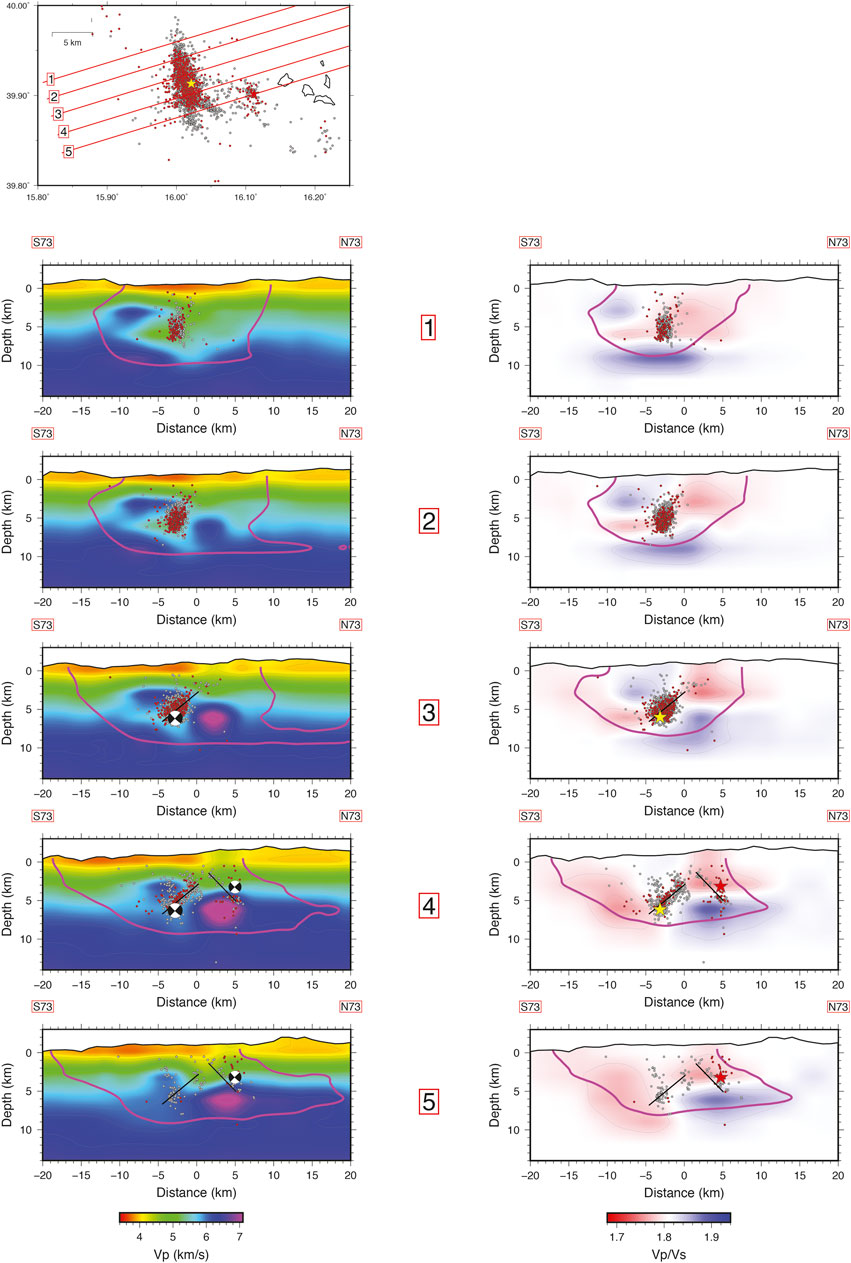
FIGURE 5. Vertical cross sections of Vp (on the left) and Vp/Vs models (on the right) across the inverted models. The traces of the five Vp and Vp/Vs vertical sections are indicated by red lines on the map in the top panel. Each trace is separated by 2.5 km, and the width for plotting earthquakes is ±1.25 km. Color scales are as indicated in Figure 4; the purple contour line represents the well resolved area in each section. Hypocenters of the relocated events occurred before and after the 25 October 2012 ML = 5.2 are represented as red and gray circles, respectively. The two main earthquakes are represented by their focal solution (http://cnt.rm.ingv.it/tdmt.html; Scognamiglio et al., 2009) on the Vp cross sections (on the left), and by red- (28 May 2012, ML = 4.3) and yellow stars (25 October 2012, ML = 5), respectively, on the Vp/Vs sections (on the right). Black line segments in Sections 3–5, on both Vp and Vp/Vs models, are the possible fault planes owing to the two main earthquakes.
Going southward, from Sections 3–5 (Figure 5, left panels), we observe that the spatial distribution of the hypocenters gradually departs from the spherical shape and starts to draw the possible fault planes where the two larger events occurred (ML=4.3, on 28 May 2012; ML=5.2 on 25 October 2012). We envisage the possible fault planes in these cross sections by black line segments, on both Vp and Vp/Vs models (Figure 5; Sections 3–5). In these sections we observe that the alignments of earthquakes cut the antiformal high velocity structure. We also observe that a very high velocity volume, up to 7.0 km/s at 6 km depth separates the alignments of hypocenters, which apparently dip in opposite direction, containing the two mainshocks of the sequence (beach balls in Sections 3–5 of Figure 5, left panels). Regarding the relationship between the relocated seismicity and the Vp/Vs., (Figure 5; Sections 3–5, right panels), we observe that the relatively low Vp/Vs areas mark the upper and the lower terminations of the main alignment of earthquakes, that containing the ML = 5.2 (yellow star in Figure 5, right panels of Sections 3, 4). In the hypothesis that this alignment draws the ruptured normal fault, higher values of Vp/Vs are found in the footwall and in the hanging wall of the fault plane. In particular, the deeper high Vp/Vs volume (Figure 5; Sections 3–5, right panels) corresponds to the highest Vp volume (up to 7 km/s) seen on the Vp tomograms (Figure 5; Sections 3–5, left panels). The smaller and less populated alignment of earthquakes containing the ML = 4.3 (red star in Figure 5, right panels of Sections 4, 5) develops in a volume of relatively low Vp/Vs, and sinks down in the high Vp/Vs volume on the bottom-east part of the model. In these southern cross sections, from 3 to 5, we observe that the ML = 5.2 fault plane was already defined by foreshocks (red circles in Figure 5, both Vp and Vp/Vs models). We also noticed that the geometry of the smaller, eastern ML = 4.3 segment is best defined by earthquakes that occurred after the ML = 5.2 (gray circles) that align on a NE dipping plane. This is likely due to the improvement of hypocentral determinations thanks to the addition of data from temporary seismic stations installed after the 25 October 2012 ML = 5.2 (see Govoni et al., 2013; Pastori et al., 2021, and references therein).
As further remarks, we observe that the distribution of the Vp/Vs ratio around the possible fault plane where the ML = 5.2 originated strongly mimics the distribution of static stress changes around a ruptured normal fault: the relatively low Vp/Vs regions, at the top and bottom tips of the fault (see Figure 5 and Sections 3, 4, and 5, right panels) corresponds to regions of expected Coulomb stress increase (e.g., Serpelloni et al., 2012, and references therein), while relatively high Vp/Vs volumes, at the foot–and hanging wall of the fault plane coincide with areas of decreasing stress. In a fluid-rich upper crustal environment, this observation can be explained by the expulsion of fluids from rock volumes subjected to increasing stress, hence pore closure, resulting into a lowering of the Vp/Vs ratio; conversely, where stress drops, rock fractures tend to open, drawing fluids from the surrounding rocks, thus increasing the Vp/Vs. Even though our tomographic model offers a static picture of the elastic properties of rocks in the faults region, the above observation supports the hypothesis that fluid-diffusion processes affected the rock volume hosting the fault system responsible for the 2010–2015 Pollino seismic swarm, as already proposed by previous studies (Passarelli et al., 2015; Napolitano et al., 2020, 2021; De Matteis et al., 2021; Sketsiou et al., 2021).
Hypocentral parameters are computed in the frame of the inversion method Simulps14q (as described above). The final location solutions are characterized by average errors of 0.11 and 0.16 km in horizontal and vertical directions, respectively. RMS of P and S travel times residuals are on average below 0.10 s.
Refined earthquake locations depict the geometry of the faults along which the two largest shocks originated. The two offset segments have a parallel NNW-strike and are elongated for 10–5 km, respectively (Figure 4). On the cross sections, the seismicity tightly defines the two clusters. Seismicity is tightly concentrated and limited by two opposite dipping faults that border a positive structure of the carbonate basement, between 3 and 7 km depth (Figure 5; Sections 3–5).
Seismicity in the western cluster, active since the end of 2011, is cloudier in the northern portion (Figure 5; Sections 1, 2), while a weak SW-dipping fault plane is visible in the southern part (Figure 5; Section 3). This plane, which becomes clearer southward (Figure 5; Sections 4, 5) was defined by seismicity also before the occurrence of the ML = 5.2 main shock (red circles in Figure 5). An antithetic E-dipping fault plane is visible to the west of the main fault, drawn by the ML = 5.2 aftershocks (gray circles in Figure 5). On the east, the hypocenters of the eastern cluster (ML = 4.3 event of May 2012) align on a NE-dipping plane (Figure 5).
Persistent swarms in the Pollino seismic gap area created concerns in public and seismic risk stakeholders, for the uncertainty on possible scenarios. Following the seismic gap hypothesis, the 2010–2015 swarms have been thought as possibly prognostic for a short term hazard increase. Previous studies of the swarm revealed its possible duplicity of roles from passive, where small patches fail around locked faults, or active, being the swarm only part of a larger aseismic release (Passarelli et al., 2015). The second scenario seems more consistent with the transient slip observed by geodetic data (Cheloni et al., 2017). The experience of the Pollino swarm could be therefore relevant to understand more in general the behavior and role of seismic swarms occurring within highly seismic areas, giving us feedback useful for hazard evaluation. In this scenario it is important to take into account recent results about CO2 flux to the area by Randazzo et al. (2022); they found values comparable to other globally significant carbon fluxes as that defined for the Himalaya orogen and Central Apennines in Italy.
The Plio-Pleistocene evolution in this transition zone has been controlled by slip on a main 110° trending strike slip shear zone (The Pollino Fault, see Spina et al., 2011; Orecchio et al., 2015; Palano et al., 2017). This fault, with a set of parallel segments and with continuation in the Ionian off-shore (the Amendolara fault, see Ferranti et al., 2014), is part of a broad lithospheric discontinuity at the edge of the retreating Ionian slab. Restraining bands along the system are observed at the meso-scale, over a large part of the fault (Figure 6). Since the Middle Pleistocene, the kinematics of the shear zone switched to extensional (Schiattarella, 1998).
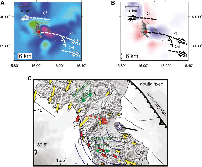
FIGURE 6. (A) Vp and (B) Vp/Vs models at 6 km depth with the system of wrench faults that originated the pop-up structure that has been re-activated and inverted during the seismic swarm. (C) GPS based velocity field (arrows), together with their 95% confidence ellipses. Euler pole is represented as a star (modified after Palano et al., 2017).
Relocated earthquakes and tomographic images reveal that seismicity developed on two main NNW-trending and opposite dipping clusters. Several studies discussed the relation with faults mapped at the surface (Brozzetti et al., 2017 and reference therein). Anyway, how the alignment of seismicity relates with the general set of faults and tectonics is not obvious. The velocity structure at depth helps clarify that seismicity is confined by antiformal pop-up structures developed in the sedimentary cover (Figure 7), buried underneath shallow thrusts of the Pollino range. We propose that the inherited compressive structure defined by tomography is part of a pop-up formed at restraining stepovers of the Pollino fault system, which left lateral sense of shear at that time, accommodated the differential SE-ward retreat of the Ionian slab. Similar structures are present at the feet of the Pollino range (Ferranti et al., 2014 and reference therein). In our model, the present day extensional seismicity, that inverted the sense of slip on the Pollino fault, reactivates and inverts the set of thrusts and back-thrusts of the pop-up structure (Figure 7). Similar reactivation of positive structures and thrusts back-thrusts systems was observed in the near val d’Agri (Buttinelli et al., 2016; Improta et al., 2017), suggesting that major strike slip faults bisected the Apulian continental margin accommodating at a large scale the differential slab retreat.
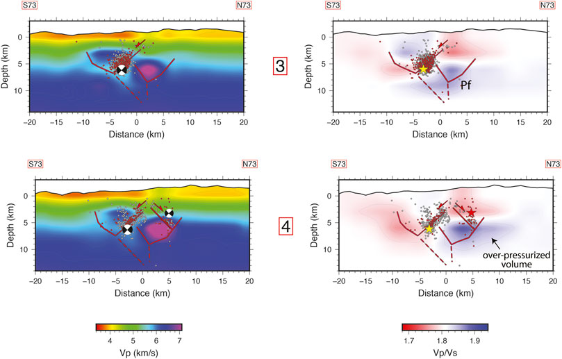
FIGURE 7. Selected vertical sections (Sections 3 and 4) of Vp and Vp/Vs with a geological sketch showing the segments of the pop-up structure (red lines) connected at depth with the Pollino fault (Pf). Hypocenter of he two major earthquakes are represented by their focal solution (http://cnt.rm.ingv.it/tdmt.html; Scognamiglio et al., 2009) on the Vp tomograms, on the left, and by red- (28 May 2012, ML = 4.3) and yellow stars (25 October 2012, ML = 5), respectively, on the Vp/Vs tomograms, on the right.
Recent models proposed that the Pollino swarm occurred in a fluid-filled high-pressure volume with triggering of events on non- optimally oriented faults (De Matteis et al., 2021). A high attenuation anomaly has been interpreted as a possible fluid accumulation at depth of 7.5 km and below that underlies the Mercure and Castrovillari sedimentary basins (Napolitano et al., 2020; Sketsiou et al., 2021). The deep high Vp/Vs observed beneath the main cluster (Figure 5, right panels) is consistent with such deep fluid volume, but the poor resolution at depths below 9 km depth precludes the reconnaissance of a broader, deeper fluid volume indicated by attenuation tomography.
Our tomographic model results from the inversion of seismic arrival times from earthquakes occurred during a 5 years time-span (2009–2013), preceding and following the two major shocks of the sequence (ML = 4.3, on 28 May 2012; ML = 5.2 on 25 October 2012). It therefore offers a static image of the crustal volume hosting that seismic sequence. Nevertheless, the strength of the Vp/Vs anomalies, and their spatial relationship with the fault segments drawn by the relocated earthquakes (see Vp/Vs tomograms in Figures 4, 5) are strong indicators that fluids are present and circulate into the imaged rock volume, thus strengthening the hypothesis that fluids diffusion processes played a relevant role in the evolution of the seismic sequence, as proposed by various authors (Passarelli et al., 2015; Napolitano et al., 2020, 2021; De Matteis et al., 2021; Sketsiou et al., 2021).
Passarelli et al. (2015) showed that the swarm-like spatial and temporal behavior of seismicity is consistent with a transient, external forcing. Accordingly, Cheloni et al. (2017) evidenced a transient slip, around the main shock, that started about 3–4 months before and lasted almost 1 year. These two inferences, together with the indirect evidence, coming from the agreement between the Vp/Vs ratio and the expected distribution of static stress changes around a ruptured normal fault (see Figure 5, right panels), that fluids can diffuse in accordance with the stress changes into the imaged crustal volume, give us the ground to hypothesize the following scenario for the swarm-like evolution of the seismic sequence:
Transient slip and associated dilation of the fault zone could have reduced pore pressures within the carbonate pop-up, accommodating aseismically a significant part of the deformation and partially inhibiting the development of a large rupture in a region where paleoseismological data suggests that larger earthquakes (Mw ≥ 6.5) may occur (Cinti et al., 2002; Tertulliani and Cucci, 2014). For undrained conditions, dilation and pre-seismic slip are directly related to pore fluid depressurization (Scuderi et al., 2015). The high Vp/Vs volume, located at the hanging wall of the fault plane (see Figure 5 and Sections 3, 4, right panels), can be the results of fluids filling fractures and cracks opened in the hanging wall during the dilatancy phase preceding the ML = 5.2 main shock (Lucente et al., 2010). In this hypothesis, before the ML = 5.2 struck, low Vp/Vs values were there where now high Vp/Vs ratio is observed, i.e. in the hanging wall of the fault. This may have resulted in a low pore fluid pressure within the carbonate rocks, concomitant with dilation and generation of slow earthquakes. The observation that foreshocks align more clearly on the ML = 5.2 fault plane and aftershocks prevail at the fault tip might suggest that the latter are mostly driven by stress changes generated by the mainshock while the effect of pore pressure is minor.
We therefore explain the space-time-magnitude pattern of the seismic sequence, and the seismicity rate, as governed by depressurization of the seismogenic volume that followed transient slip. According with theoretical modeling and laboratory experiments (Wang and Nur, 1989; Dvorkin et al., 1999; Vanorio et al., 2005), low Vp/Vs anomalies are indicative of low pore pressure within fluid-saturated rock volumes since the closing of pores and cracks significantly modifies the shear wave velocity. A low pore pressure within the swarm volume is consistent with a local stressing of small patches, as also observed for other tectonic seismic swarms (De Gori et al., 2015).
The Pollino seismic gap hypothesis derives from tectonic models that assume a continuity in deformation between the southern Apennines and the Calabrian arc and is motivated by the absence of large earthquakes in historical records (Rovida et al., 2016) in an area which spans across the Pollino mountain range, to the North, and spreads to the upper Crati valley, to the South, for about 60 km.
Paleo-seismological investigation across faults at the southern border of the Pollino range revealed the traces of ancient, large slip, earthquakes, older than 1 Kyr (Michetti et al., 1997; Cinti et al., 2002), demonstrating that large earthquakes have happened in the past, and are therefore possible to occur in this region.
Recent evidence emerged for the Pollino wrench fault acting as a major heterogeneity, supporting a kinematic decoupling between the Apennines and Calabrian blocks (Chiarabba et al., 2016; Palano et al., 2017). In this line of view, the 2010–2014 seismic swarm struck within such a complex transfer zone (Figure 6).
The absence of large earthquakes in the historical catalog has been associated with a combination of low strain rate and mixed seismic/aseismic strain release that could increase the recurrence time of large magnitude events (Cheloni et al., 2017).
Our results demonstrate that fluid diffusion processes are likely to occur in this area, with the potential to drive the seismicity, favoring the release of the stress through microseismicity. Furthermore, the feeble extension of less than 2 mm/yrs across the ridge slowly loads the faults, and is partially ineffective for their reactivation and inversion. The inherited geometry of the pop-up structure is the more likely cause of fault segmentation in the seismic gap area, that leads to fault segments with a maximum length in the order of 10–15 km. Moreover, the Pollino fault also acts as a further segmentation of the system, bounding segments connected with the Apennines extension to the north (the last of which being those activated during the swarm) and those with the Crati valley extension to the south (Ferranti et al., 2014, and references therein).
The 4-years long seismic swarm strucking the northern portion of the Pollino seismic gap developed on fault segments in the shallow crust. Such segments were formerly part of a compressive pop-up structure formed at a restraining band of the Pollino wrench fault, and are now re-activated in extension. The evidence for the presence of fluids within the seismogenic volume suggests that fluid diffusion processes may have influenced the evolution of the seismic sequence in a swarm-like behavior, accompanying and favoring a 1-year long transient aseismic slip.
The waveform data of earthquakes used in this study are archived in EIDA, waveform database https://eida.ingv.it/en/. The used stations are mainly from the Italian National Seismic Network (doi.org/10.13127/SD/X0FXnH7QfY).
PD analyzed the data and evaluated the Vp and Vp/Vs tomography and wrote the manuscript; FPL analyzed the data draw the figures discussed the results and wrote the manuscript; AG installed and maintained the temporary stations in the field, made data available and helped in the discussion; LM coordinated the working group helped in the discussion and wrote the manuscript, CC discussed the results and wrote the manuscript.
This study has benefited from funding provided by the Italian Presidenza del Consiglio dei Ministri—Dipartimento della Protezione Civile (DPC). This paper does not necessarily represent DPC official opinion and policies.
We would like to thank Milena Moretti and the other INGV personnel working to collect the data of temporary and permanent seismic stations. We would like to follow up by thanking all the INGV staff on shifts in the surveillance room in Rome for their work and the Bollettino Sismico Italiano working group (http://terremoti.ingv.it/bsi) and the authors of the paper Pastori et al., 2021, for making available the files of the manually revised P- and S-phase pickings. We are grateful for the comments and suggestions of the Guest Associated Editor Federica Lanza and the two reviewers, which helped us to improve the final version of the manuscript.
The authors declare that the research was conducted in the absence of any commercial or financial relationships that could be construed as a potential conflict of interest.
All claims expressed in this article are solely those of the authors and do not necessarily represent those of their affiliated organizations, or those of the publisher, the editors and the reviewers. Any product that may be evaluated in this article, or claim that may be made by its manufacturer, is not guaranteed or endorsed by the publisher.
Bachura, M., Fischer, T. J. Doubravová, Horálek, J., and Horalek, J. (2021). From earthquake swarm to a mainshock–aftershocks: The 2018 activity in west bohemia/vogtland. Geophys. J. Int. 224 (3), 1835–1848. doi:10.1093/gji/ggaa523
Bigi, G., Bonardini, G., Catalano, R., Cosentino, D., Lentini, F., Parlotto, M., et al. (1992). Structural model of Italy, 1:500.000. Rome: Consiglio Nazionale delle Ricerche.
Brozzetti, F., Cirillo, D., de Nardis, R., Cardinali, M., Lavecchia, G., Orecchio, B., et al. (2017). Newly identified active faults in the Pollino seismic gap, southern Italy, and their seismotectonic significance. J. Struct. Geol. 94, 13–31. doi:10.1016/j.jsg.2016.10.005
Brozzetti, F., Lavecchia, G., Mancini, G., Milana, G., and Cardinali, M. (2009). Analysis of the 9 september 1998 Mw 5.6 mercure earthquake sequence (southern Apennines, Italy): A multidisciplinary approach. Tectonophysics 476, 210–225. doi:10.1016/j.tecto.2008.12.007
Brozzetti, F. (2011). The campania-lucania extensional fault system, southern Italy: A suggestion for a uniform model of active extension in the Italian Apennines. Tectonics 30, TC5009doi. doi:10.1029/2010TC002794
Buttinelli, M., Improta, L., Bagh, S., and Chiarabba, C. (2016). Inversion of inherited thrusts by wastewater injection induced seismicity at the Val d'Agri oilfield (Italy). Sci. Rep. 6 (1), 37165. doi:10.1038/srep37165
Cheloni, D., D'Agostino, N., Selvaggi, G., Avallone, A., Fornaro, G., Giuliani, R., et al. (2017). Aseismic transient during the 2010-2014 seismic swarm: Evidence for longer recurrence of M ≥ 6.5 earthquakes in the Pollino gap (southern Italy)? Sci. Rep. 7 (576), 576. doi:10.1038/s41598-017-00649-z
Chiarabba, C., Agostinetti, N. P., and Bianchi, I. (2016). Lithospheric fault and kinematic decoupling of the Apennines system across the Pollino range. Geophys. Res. Lett. 43, 3201–3207. doi:10.1002/2015GL067610
Chiarabba, C., Buttinelli, M., Cattaneo, M., and De Gori, P. (2020). Large earthquakes driven by fluid overpressure: The Apennines normal faulting system case. Tectonics 39 (4), e2019TC006014. doi:10.1029/2019tc006014
Chiarabba, C., De Gori, P., and Speranza, F. (2008). The southern Tyrrhenian subduction zone: Deep geometry, magmatism and Plio-Pleistocene evolution. Earth Planet. Sci. Lett. 268, 408–423. doi:10.1016/j.epsl.2008.01.036
Chiarabba, C., Jovane, L., and Di Stefano, R. (2005). A new view of Italian seismicity using 20 years of instrumental recordings. Tectonophysics 395, 251–268. doi:10.1016/j.tecto.2004.09.013
Chiarabba, C., Piccinini, D., and De Gori, P. (2009). Velocity and attenuation tomography of the umbria marche 1997 fault system: Evidence of a fluid-governed seismic sequence. Tectonophysics 4761-2, 73–84. doi:10.1016/j.tecto.2009.04.004
Cinti, F. R., Cucci, L., Pantosti, D., D’addezio, G., and Meghraoui, M. (1997). A major seismogenic fault in a “silent area”: the.Castrovillari fault (southern Apennines, Italy). Geophys. J. Int. 130, 595–605. doi:10.1111/j.1365-246x.1997.tb01855.x
Cinti, F. R., Moro, M., Pantosti, D., Cucci, L., and D’addezio, G. (2002). New constraints on the seismic history of the Castrovillari fault in the Pollino gap (Calabria, southern Italy). J. Seismol. 6, 199–217. doi:10.1023/a:1015693127008
Cirillo, D., Totaro, C., Lavecchia, G., Orecchio, B., de Nardis, R., Presti, D., et al. (2022). Structural complexities and tectonic barriers controlling recent seismic activity in the Pollino area (Calabria–Lucania, southern Italy) – constraints from stress inversion and 3D fault model building. Solid earth. 13, 205–228. doi:10.5194/se-13-205-2022
D’Agostino, N., D’Agostino, N., D’Anastasio, E., Gervasi, A., Guerra, I., Nedimovic, M. R., Seeber, L., et al. (2011). Forearc extension and slow rollback of the Calabrian Arc from GPS measurements. Geophys. Res. Lett. 38 (17). doi:10.1029/2011GL048270
D’Agostino, N., and Selvaggi, G. (2004). Crustal motion along the eurasia-nubia plate boundary in the Calabrian arc and sicily and active extension in the messina straits from GPS measurements. J. Geophys. Res. 109, B11402. doi:10.1029/2004JB002998
De Barros, L., Cappa, F., Deschamps, A., and Dublanchet, P. (2020). Imbricated aseismic slip and fluid diffusion drive a seismic swarm in the Corinth Gulf, Greece. Geophys. Res. Lett. 47, e2020GL087142. doi:10.1029/2020GL087142
De Gori, P., Lucente, F. P., and Chiarabba, C. (2015). Stressing of fault patch during seismic swarms in central Apennines, Italy. Geophys. Res. Lett. 42, 2157–2163. doi:10.1002/2015GL063297
De Matteis, R., Convertito, V., Napolitano, F., Amoroso, O., Terakawa, T., and Capuano, P. (2021). Pore fluid pressure imaging of the Mt. Pollino region (southern Italy) from earthquake focal mechanisms. Geophys. Res. Lett. 48, e2021GL094552. doi:10.1029/2021GL094552
Di Stefano, R., Kissling, E., Chiarabba, C., Amato, A., and Giardini, D. (2009). Shallow subduction beneath Italy: Three-dimensional images of the Adriatic-European-Tyrrhenian lithosphere system based on high-quality P wave arrival times. J. Geophys. Res. 114, B05305. doi:10.1029/2008JB005641
Dvorkin, J., Mavko, G., and Nur, A. (1999). Overpressure detection from compressional- and shear-wave data. Geophys. Res. Lett. 26, 3417–3420. doi:10.1029/1999gl008382
Faccenna, C., Funiciello, F., Giardini, D., and Lucente, F. P. (2001). Episodic back-arc extension during restricted mantle convection in the Central Mediterranean. Earth Planet. Sci. Lett. 187 (1-2), 105–116. doi:10.1016/s0012-821x(01)00280-1
Faccenna, C., Piromallo, C., CrespoBlanc, A., Jolivet, L., and Rossetti, F. (2004). Lateral slab deformation and the origin of the Western Mediterranean arcs. Tectonics 23, TC1012. doi:10.1029/2002TC001488
Ferranti, L., Burrato, P., Pepe, F., Santoro, E., Mazzella, M. E., Morelli, D., et al. (2014). An active oblique‐contractional belt at the transition between the Southern Apennines and Calabrian Arc: The Amendolara Ridge, Ionian Sea, Italy. Tectonics 33 (11), 2169–2194.
Giacomuzzi, G., Civalleri, M., De Gori, P., and Chiarabba, C. (2012). A 3D vs model of the upper mantle beneath Italy: Insight on the geodynamics of central Mediterranean. Earth Planet. Sci. Lett. 335, 105–120. doi:10.1016/j.epsl.2012.05.004
Govoni, A., Passarelli, L., Braun, T., Maccaferri, F., Moretti, M., Lucente, F. P., et al. (2013). Investigating the origin of seismic swarms. Eos Trans. AGU. 94 (41), 361–362. doi:10.1002/2013eo410001
Gruppo di Lavoro, M. P. S. (2004). “Redazione della mappa di pericolosità sismica prevista dall'Ordinanza PCM 3274 del 20 marzo 2003,” in Rapporto conclusivo per il Dipartimento della Protezione civile (Milano-Roma: INGVaprile), 65. + 5 appendici.
Hardebeck, J. L., Felzer, K. R., and Michael, A. J. (2008). Improved tests reveal that the accelerating moment release hypothesis is statistically insignificant. J. Geophys. Res. 113, B08310. doi:10.1029/2007JB005410
Haslinger, F. (1998). Velocity structure, seismicity and seismotectonics of northwestern Greece between the gulf of arta and zakynthos. PhD thesis. Zurich: ETH, 176.
Holtkamp, S., and Brudzinski, M. R. (2014). Megathrust earthquake swarms indicate frictional changes which delimit large earthquake ruptures. Earth Planet. Sci. Lett. 390, 234–243. doi:10.1016/j.epsl.2013.10.033
Improta, L., Bagh, S., de Gori, P., Valoroso, L., Pastori, M., Piccinini, D., et al. (2017). Reservoir structure and wastewater-induced seismicity at the val d'Agri oilfield (Italy) shown by three-DimensionalVpandVp/VsLocal earthquake tomography. J. Geophys. Res. Solid Earth 122, 9050–9082. doi:10.1002/2017JB014725
Improta, L., Iannaccone, G., Capuano, P., Zollo, A., and Scandone, P. (2000). Inferences on the upper crustal structure of Southern Apennines (Italy) from seismic refraction investigations and subsurface data. Tectonophysics 317, 273–298. doi:10.1016/s0040-1951(99)00267-x
Ito, Hisao, DeVilbiss, John, and Nur, Amos (1979). Compressional and shear waves in saturated rock during water‐steam transition. J. Geophys. Res. Solid Earth 84, 4731–4735. doi:10.1029/JB084iB09p04731
Lucente, F. P., De Gori, P., Margheriti, L., Piccinini, D., Di Bona, M., Chiarabba, C., et al. (2010). Temporal variation of seismic velocity and anisotropy before the 2009 MW6.3 L'Aquila earthquake, Italy. Geology 38 (11), 1015–1018. doi:10.1130/g31463.1
Lucente, F. P., Margheriti, L., Piromallo, C., and Barruol, G. (2006). Seismic anisotropy reveals the long route of the slab through the Western-central Mediterranean mantle. Earth Planet. Sci. Lett. 241, 517–529. doi:10.1016/j.epsl.2005.10.041
Margheriti, L., Amato, A., Braun, T., Cecere, G., D'Ambrosio, C., De Gori, P., et al. (2013). Emergenza nell’area del Pollino: Le attività della Rete sismica mobile. Rapporti tecnici INGV 252. Available at: http://editoria.rm.ingv.it/archivio_pdf/rapporti/251/pdf/rapporti_252.pdf.
Michelini, A., and McEvilly, T. V. (1991). Seismological studies at Parkfield, I, Simultaneous inversion for velocity structure and hypocentres using cubic b-splines parameterization. Bull. Seismol. Soc. Am. 81, 524–552. doi:10.1785/BSSA0810020524
Michetti, A. M., Ferreli, L., Serva, L., and Vittori, E. (1997). Geological evidence for strong historical earthquakes in an “aseismic” region: The Pollino case (southern Italy). J. Geodyn. 24, 67–86. doi:10.1016/s0264-3707(97)00018-5
Napolitano, F., Amoroso, O., La Rocca, M., Gervasi, A., Gabrielli, S., and Capuano, P. (2021). Crustal structure of the seismogenic volume of the 2010–2014 Pollino (Italy) seismic sequence from 3D P-and S-wave tomographic images. Front. Earth Sci. (Lausanne). 9. doi:10.3389/feart.2021.735340
Napolitano, F., De Siena, L., Gervasi, A., Guerra, I., Scarpa, R., and La Rocca, M. (2020). Scattering and absorption imaging of a highly fractured fluid-filled seismogenetic volume in a region of slow deformation. Geosci. Front. 11 (3), 989–998. doi:10.1016/j.gsf.2019.09.014
Napolitano, F., Galluzzo, D., Gervasi, A., Scarpa, R., and La Rocca, M. (2021). Fault imaging at Mt Pollino (Italy) from relative location of microearthquakes. Geophys. J. Int. 224, 637–648. doi:10.1093/gji/ggaa407
Nur, A. (1972). Dilatancy, pore fluids, and premonitory variations of travel times: Seismological Society of America Bulletin, 78, p. 1217–1222. doi:10.1785/BSSA0620051217
Orecchio, B., Presti, D., Totaro, C., D’Amico, S., and Neri, G. (2015). Investigating slab edge kinematics through seismological data: The northern boundary of the Ionian subduction system (south Italy). J. Geodyn. 88, 23–35. doi:10.1016/j.jog.2015.04.003
Palano, M., Piromallo, C., and Chiarabba, C. (2017). Surface imprint of toroidal flow at retreating slab edges: The first geodetic evidence in the calabrian subduction system. Geophys. Res. Lett. 44, 845–853. doi:10.1002/2016gl071452
Passarelli, L., Hainzl, S., Cesca, S., Maccaferri, F., Mucciarelli, M., Roessler, D., et al. (2015). Aseismic transient driving the swarm-like seismic sequence in the Pollino range, Southern Italy. Geophys. J. Int. 201 (3), 1553–1567. doi:10.1093/gji/ggv111
Pastori, M., Margheriti, L., De Gori, P., Govoni, A., Lucente, F. P., Moretti, M., et al. (2021). The 2011–2014 Pollino seismic swarm: Complex fault systems imaged by 1D refined location and shear wave splitting analysis at the Apennines–Calabrian arc boundary. Front. Earth Sci. 9, 618293. doi:10.3389/feart.2021.618293
Piana Agostinetti, N., and Amato, A. (2009). Moho depth andVp/Vsratio in peninsular Italy from teleseismic receiver functions. J. Geophys. Res. 114, B06303. doi:10.1029/2008JB005899
Piana Agostinetti, N., Steckler, M. S., and Lucente, F. P. (2009). Imaging the subducted slab under the Calabrian Arc, Italy, from receiver function analysis. Lithosphere 1, 131–138. doi:10.1130/L49.1
Randazzo, P., Caracausi, A., Aiuppa, A., Cardellini, C., Chiodini, G., Apollaro, C., et al. (2022). Active degassing of crustal CO2 in areas of tectonic collision: A case study from the Pollino and Calabria sectors (southern Italy). Front. Earth Sci. 10, 946707. doi:10.3389/feart.2022.946707
Ross, Z. E., Cochran, E. S., Trugman, D. T., and Smith, J. D. (2020). 3D fault architecture controls the dynamism of earthquake swarms. Science 368 (6497), 1357–1361. doi:10.1126/science.abb0779
Rovida, A., Locati, M., Camassi, R., Lolli, B., and Gasperini, P. (Editors) (2016). CPTI15, the 2015 version of the parametric catalogue of Italian earthquakes (Istituto Nazionale di Geofisica e Vulcanologia). doi:10.6092/INGV.IT-CPTI15
Schiattarella, M. (1998). “Quaternary tectonics of the Pollino ridge, calabria-lucania boundary, southern Italy,”. Editor R. E. R. A. J. F. HoldsworthStrachanDewey (London: Geol. Soc. Lond.), 135, 341–354.Cont. transpressional transtensional Tect. Spec. Publ.
Scognamiglio, L., Tinti, E., and Michelini, A. (2009). Real-time determination of seismic moment tensor for the Italian region. Bull. Seismol. Soc. Am. 99 (4), 2223–2242. doi:10.1785/0120080104
Scuderi, M. M., Carpenter, B. M., Johnson, P. A., and Marone, C. (2015). Poromechanics of stick-slip frictional sliding and strength recovery on tectonic faults. J. Geophys. Res. Solid Earth 120, 6895–6912. doi:10.1002/2015JB011983
Serpelloni, E., Anderlini, L., and Belardinelli, M. E. (2012). Fault geometry, coseismic-slip distribution and Coulomb stress change associated with the 2009 April 6, M w 6.3, L′ Aquila earthquake from inversion of GPS displacements. Geophys. J. Int. 1882, 473–489. doi:10.1111/j.1365-246x.2011.05279.x
Sketsiou, P., De Siena, L., Gabrielli, S., and Napolitrano, F. (2021). 3-D attenuation image of fluid storage and tectonic interactions across the Pollino fault network. Geophys. J. Int. 226, 536–547. doi:10.1093/gji/ggab109
Spina, V., Tondi, E., and Mazzoli, S. (2011). Complex basin development in a wrench-dominated back-arc area: Tectonic evolution of the Crati Basin, Calabria, Italy. J. Geodyn. 51, 90–109. doi:10.1016/j.jog.2010.05.003
Tertulliani, A., and Cucci, L. (2014). New insights on the strongest historical earthquake in the Pollino region (southern Italy). Seismol. Res. Lett. 85, 743–751. doi:10.1785/0220130217
Thurber, Clifford H., and Atre, Shashank R. (1993). Three-dimensional vp/vs variations along the loma prieta rupture zone. Bull. Seismol. Soc. Am. 833, 717–736.
Toomey, D. R., and Foulger, G. R. (1989). Tomographic inversion of local earthquake data from the Hengill–Grensdalur central volcano complex, Iceland. J. Geophys. Res. 94 (12), 17497. doi:10.1029/jb094ib12p17497
Totaro, C., Koulakov, I., Orecchio, B., and Presti, D. (2014). Detailed crustal structure in the area of the southern Apennines–Calabrian Arc border from local earthquake tomography. J. Geodyn. 82, 87–97. doi:10.1016/j.jog.2014.07.004
Totaro, C., Presti, D., Billi, A., Gervasi, A., Orecchio, B., Guerra, I., et al. (2013). The ongoing seismic sequence at the Pollino Mountains Italy. Seismol. Res. Lett. 84 (6), 955–962. doi:10.1785/0220120194
Vanorio, T., Virieux, J., Capuano, P., and Russo, G. (2005). Three-dimensional seismic tomography from P-wave and S- wave microearthquake travel times and rock physics characterization of the Campi Flegrei Caldera. J. Geophys. Res. 110, B03201. doi:10.1029/2004JB003102
Wang, Z., and Nur, A. M. (1989). Effects of CO2 flooding on wave velocities in rocks with hydrocarbons. SPE Reserv. Eng. 3, 429–436. doi:10.2118/17345-pa
Wu, C., Meng, X., Peng, Z., and Ben-Zion, Y. (2014). Lack of spatiotemporal localization of foreshocks before the 1999 Mw 7.1 Düzce, Turkey, earthquake. Bull. Seismol. Soc. Am. 104 (1), 560–566. doi:10.1785/0120130140
Zhang, G., Lei, J., and Sun, D. (2019). The 2013 and 2017 Ms 5 seismic swarms in Jilin, NE China: Fluid-triggered earthquakes? J. Geophys. Res. Solid Earth 124, 13096–13111. doi:10.1029/2019JB018649
Keywords: seismic swarm, seismic gap, earthquake location, tomographic model, fault weakening, pop-up structures, seismic hazard
Citation: De Gori P, Lucente FP, Govoni A, Margheriti L and Chiarabba C (2022) Seismic swarms in the Pollino seismic gap: Positive fault inversion within a popup structure. Front. Earth Sci. 10:968187. doi: 10.3389/feart.2022.968187
Received: 13 June 2022; Accepted: 27 October 2022;
Published: 10 November 2022.
Edited by:
Federica Lanza, ETH Zurich, SwitzerlandReviewed by:
Ferdinando Napolitano, University of Salerno, ItalyCopyright © 2022 De Gori, Lucente, Govoni, Margheriti and Chiarabba. This is an open-access article distributed under the terms of the Creative Commons Attribution License (CC BY). The use, distribution or reproduction in other forums is permitted, provided the original author(s) and the copyright owner(s) are credited and that the original publication in this journal is cited, in accordance with accepted academic practice. No use, distribution or reproduction is permitted which does not comply with these terms.
*Correspondence: Lucia Margheriti, bHVjaWEubWFyZ2hlcml0aUBpbmd2Lml0
Disclaimer: All claims expressed in this article are solely those of the authors and do not necessarily represent those of their affiliated organizations, or those of the publisher, the editors and the reviewers. Any product that may be evaluated in this article or claim that may be made by its manufacturer is not guaranteed or endorsed by the publisher.
Research integrity at Frontiers
Learn more about the work of our research integrity team to safeguard the quality of each article we publish.