
95% of researchers rate our articles as excellent or good
Learn more about the work of our research integrity team to safeguard the quality of each article we publish.
Find out more
ORIGINAL RESEARCH article
Front. Earth Sci. , 05 January 2023
Sec. Geochemistry
Volume 10 - 2022 | https://doi.org/10.3389/feart.2022.963290
This article is part of the Research Topic Reservoir Formation Conditions and Enrichment Mechanisms of Shale Oil and Gas View all 48 articles
 Chaoqian Zhang1†Yongle Hu1Suwei Wu1
 Mingming Tang2*†Kexin Zhang1Heping Chen1Xuepeng Wan3Wensong Huang1Di Han1Zheng Meng1
Due to the dual effects of fluvial and tides, the tidal sand bars in estuaries have complex sedimentary characteristics and complex internal structures, making them difficult to predict and describe. In this paper, the sedimentary dynamics numerical simulation method is used to establish a tidal-controlled estuary model. The effects of tidal range and sediment grain size on tidal sand bars are simulated. The length, width, and thickness of tidal sand bars, as well as the length and thickness of the internal shale layer, are also analyzed. The results show that in the environment of a tide-controlled estuary, the tidal range has a more significant effect on tidal sand bars compared to the sediment grain size under the specific conditions used in this study. The main effect of tidal range on tidal sand bars is that the greater the tidal range, the greater the length-to-width ratio of the sandbank, and the higher the degree of sandbank development. In a tidal-controlled estuary environment, the formation and distribution of shale layer structures are also affected by tides: the length of the shale layer increases as the tidal energy increases, but the changes in the thickness are not obvious. Numerical simulations of the development and distribution of the tidal sand bars and shale layers in estuaries based on sedimentary dynamics will provide a basis for the sedimentary evolution of tide-controlled estuaries and will provide guidance for the exploration and development of tidal estuaries.
The Oriente Basin is located in the transition zone between the active Cordillera mountain system of South America and the stable Gondwana shield (Zhang et al., 2018; Ma et al., 2020). It is located in the northeast of Ecuador, has a north–south trend, and is steep in the west and gentle in the east. It is part of the foreland basin. The Oriente Basin has nearly 30 billion barrels worth of oil reserves, accounting for 97% of Ecuador’s proven reserves, and is one of the most abundant basins in the northwest basin chain of South America (Yang et al., 2018). The strata of the Oriente Basin include sediments from the Phanerozoic Paleozoic to Quaternary eras (Toffolon and Crosato, 2007; Fan and Shang, 2014). The basin is composed of two sets of large sequences of metamorphic rock basements with sedimentary filling, and the sedimentary strata can be divided into three parts from bottom to top: a pre-Cretaceous basement sedimentary layer, a Cretaceous sedimentary layer consisting of continental facies and an intersecting shallow sea, and post-Cretaceous continental foreland strata. The main oil-producing strata in the Oriente Basin are Cretaceous, including the Hollin formation, which is Lower Cretaceous, and the Napo formation and Tena formation, which are Upper Cretaceous. From the Hollin formation to the Napo formation, transgression occurred from west to east followed by regression, and the Tena formation was deposited. In the Upper Cretaceous Napo formation, the main rock sources are marine black shale and asphaltene carbonate rock, while the main reservoirs of the Napo formation are composed of stacked tidal-controlled estuary sediment formations (Jaillard et al., 2006).
The earliest definition of an estuary was put forward by Pritchard, who defined an estuary as a semi-closed coastal water body where the salinity is significantly diluted by fresh water from the land, with salinity levels ranging from 0.1‰ to 30–35‰ (Pritchard, 1955). The definition is based on the salinity of the water body, but the specific geological or stratigraphic information is ignored, so there is limited information for the study of estuarine sediments. Fairbridge considered the importance of tidal action on estuaries and proposed that estuaries be defined as: “the upper limit of the passage of the ocean into the valley is the limit of tidal surge” (Fairbridge, 1980). However, the scope of this definition is not limited to estuaries and is also applicable to deltas and lagoons. Dalrymple put forward a “geological” definition of estuaries, believing that “the estuary is the submerged part of the incised valley system, receiving sediments from rivers and oceans, including sedimentary facies affected by tides, waves and rivers” (Dalrymple et al., 1992). This definition takes the incised valley system as a necessary condition for the formation of estuaries, but estuaries can also form transgressive parts with delta plains; transgression, sufficient sedimentary space, and the land transport of sediments are more important for the formation of an estuary. Dalrymple put forward a new definition of estuaries in 2006. He believed that an “estuary is the offshore part of drowning valley system, which receives sediments from rivers and oceans, and also contains sedimentary facies affected by tides, waves and rivers. The top of the bay is the upper limit of tidal facies sediment distribution, and the mouth of the bay is the lower limit of coastal facies sediment distribution”, and this definition is widely accepted (Dalrymple et al., 1992). At present, the most widely used methods used to study tidal-controlled estuary deposits include estuary outcrop field survey, modern deposition example anatomy, seismic data, and logging curve interpretation analysis (Dalrymple and Choi, 2007; Reisinger et al., 2017; Xie et al., 2018; Zheng et al., 2018). In paleo sedimentary fields, outcrops are very rare, furthermore, they can only provide two-dimensional structural information, and the information on the internal three-dimensional structure is insufficient; it is difficult to determine the anatomy of modern sedimentary examples, and this method is suitable for observing delta deposits and inland estuary deposits at low tide. Areas that are buried underwater are not easy to observe, and the resolution of seismic data is relatively limited (Jaillard et al., 2006). In this paper, the sedimentary dynamics numerical simulation method is used to set different tidal ranges and sediment grain sizes to carry out sedimentation simulations of the tidal-controlled estuary bar and its shale layer and to explore the effects of the controlling factors on tidal bar development and distribution. By analyzing the development characteristics of the length, width, and thickness of the bar, the relationship between each factor and the sedimentary characteristics of the estuary sand bar is revealed.
The sedimentary dynamics method, also known as sedimentation simulation technology, is a reservoir description and prediction technology that was originally developed based on hydrodynamics and sedimentology. It quantitatively simulates the real clastic sedimentary system in nature on the scales of time and space and follows a series of physical laws, such as the law of conservation of energy. Sedimentary numerical simulation relies on computer technology and uses numerical calculation methods to solve fluid mechanics equations using a computer, thereby simulating the natural phenomena and geomorphological evolution process of the research object (Lageweg and Feldman, 2018). Numerical simulations have repeatability, operability, and variability of simulation factors. They can simulate sedimentary morphology in any environment according to various conditions and can quickly calculate the simulation results in a large time and space range. It is used to analyze the sedimentation of estuaries. The sedimentary characteristics under these factors are convenient.
Advances in computer technology have promoted the rapid development of sedimentary numerical simulation. The study of sedimentary numerical simulation began in the 1960s. At first, the entire geological sedimentation process was converted into simulated numerical values and then into computer numerical codes. By the 1980s, there had been more two-dimensional numerical simulation studies carried out abroad, and gradually, numerical simulation was applied to the study of topography and geomorphology (Van and Feldman, 2018). The most representative numerical model is 2DH; in the 1990s, people began to study three-dimensional numerical simulation, and three-dimensional hydrodynamic models based on the Navier–Stokes equations began to be established; after the 21st century, as the production needs of the petroleum industry intensified, numerical simulation began to be used in sedimentary research. Nowadays, many experts and scholars both at home and abroad apply numerical simulations of sedimentary dynamics to the sedimentation in estuaries. Schramkowski et al. (2002) conducted a numerical simulation of tidal-controlled estuaries in; Toffolon and Crosato (2007) studied tide control and specifically focused on the shape of the sand bar in the selected estuary; Lageweg et al. (2018) simulated the flow and tidal amplitude factors in a tidal-controlled estuary; Weisscher et al. (2019) published the use of Nays2D sedimentation numerical simulation software for morphological dynamic modeling to determine the impact of dynamic inflow disturbances on river patterns and dynamic meandering rivers. And Tang et al. (2019) used numerical simulation to study the reservoir configuration of tidal-controlled estuaries. This paper adopts Tang et al.'s sedimentation simulation model (Tang et al., 2019).
In the above equations, U and V represent the average velocity of the fluid in the x and y directions, respectively; t represents the time; u, v, and ω represent the flow velocity in the x, y, and z directions; h represents the total depth of the water body; f represents Corio; ρ0 represents the reference density of the water; σ represents the reduction ratio according to the ordinate; Px and Py represent the horizontal pressure items approximated by Boussinesq; Fx and Fy represent the horizontal Reynolds stress determined by the concept of vortex viscosity; Mx and My represent water consumption; ζ represents the height difference between the free surface and the reference surface (z=0); S represents the model surface area; c represents the mass concentration; DH represents the horizontal eddy diffusion rate; DV represents the vertical eddy diffusion coefficient of the transport equation; and c(ι)represents the fraction of sediment mass concentration.
The sediment components mainly consist two types: cohesive and non-cohesive components. The cohesive sediment component is controlled by the suspended-transport equation, while the non-cohesive sediment component is partly in suspension and partly through bed load. For cohesive sediment components, the fluxes between the water phase and the bed are calculated with the well-known Partheniades-Krone formulations (Eqs. 6,7) (Caldwell and Edmonds, 2014). Based on this equation, the sediment transport for bedload could be calculated directly.
Where
The simulated estuary shape is characterized by an ideal funnel shape (Figure 1). The model domain is 36km×100km, and consists equal grids with a resolution of 200 m by 160 m. The time step of 100 min is selected to ensure stability and accuracy. The maximum bed shear stress
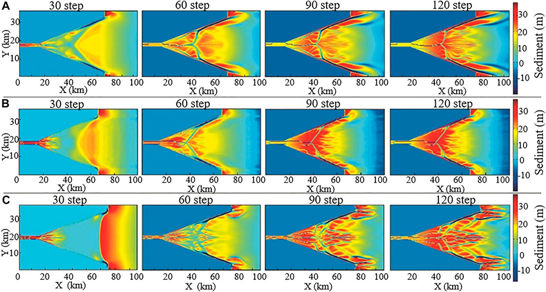
FIGURE 1. Sediment thickness of the estuary at different tide heights (A) represents the tide at 3.4 m, (B) represents the tide at 6.8 m, and (C) represents the tide at 7.2 m).
The ebb tide increases as the tidal range increases. The simulation results of a tidal-controlled estuary indicate that the shape of the sand bar changes significantly as the tidal range changes (Figure 1). When the intensity of the tide is small, the tidal range is 3.4 m (Figure 1A), the sediment accumulation range is small, and the degree of development of the sand bars in the estuary is not high, but the thickness of the sand bars is the largest, with an average thickness of 24.5 m. When the height of the tidal range increases to 6.8m and 7.2m, the sand bars have a high degree of sedimentation along the outer estuary. At this time, the tidal sand bars and tidal channels are more developed. Under the conditions of a medium tidal range (Figure 1B) or a large tidal range (Figure 1C), the sand bars are eroded and redeposited, and the sand bars in the outer river mouth are long strips. These results here are in a very good agreement with those in the literatures (Billy et al., 2012; Alam, 2014). The greater the tidal range, the greater the receding tide, the greater the degree of sediment diffusion, the higher the degree of sand bar cutting by the tidal channel, and the larger the number of sand bars.
Simulations of the sediment grain size were carried out to change the size of the sand. The model was divided into fine-grained sizes, medium-grained sizes, and coarse-grained sizes. There were three types of sediment grains for each case. The sediment grain sizes for the fine-grained size model were 80 μm, 64 μm, and 60 μm. Additionally, the sediment grain sizes for the medium-grained size model were 125 μm, 80 μm, and 64 μm, and the sediment grain sizes for the coarse-grained size model were 250 μm, 125 μm, 80 μm. As shown in Figure 2, changing sediment grain size does not affect the deposition rate of the estuary bar, and the deposition rate of the estuary bar under the three grain sizes is roughly the same. At the beginning of the simulation, the fine-grained sediments were transported far away, and there was obvious bar deposition in the middle of the estuary. At the end of the simulation, there was obvious strip deposition at the top of the estuary under medium- and coarse-grained conditions. As the simulation of the fine-grained and medium-grained estuarine models developed, sand and shale were deposited in the inner estuarine, forming sheet deposits. The channel mainly developed in the middle of the river. The tidal sand bar is in the shape of fine strips, and the segmentation of the sand bar is not obvious, which is agreed with the results proposed by Poppeschi et al. (2021) and Grasso et al. (2021). In the coarse-grained estuarine model, there are many rivers in the inner-river estuary, the curvature of tidal channel is higher, and the sand bar segmentation is stronger.
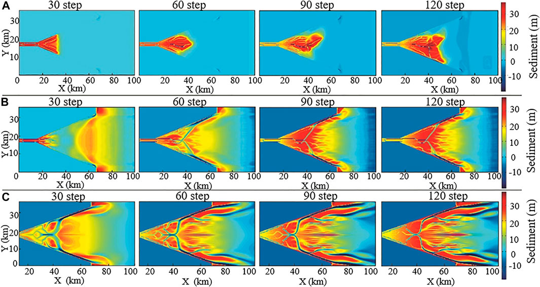
FIGURE 2. Sediment thickness of the estuary under different sediment grain size conditions (A): fine-grained size model, (B) medium-grained size model, (C) coarse-grained size model).
Changes in the external environment cause different sedimentary forms in tidal-controlled estuaries. The developmental law of tidal-controlled estuaries is controlled by many factors. At the same time, the distribution of the shale layers inside sand bars also changes with changes in various factors. The length-to-width ratio of sand bars can reflect the primary and secondary factors that control the shape of sand bars in tidal-controlled estuaries. By comparing the length-to-width ratio of sand bars, the main controlling factors that control the development of the sand bars in tidal-controlled estuaries are obtained to provide a theoretical basis for research on the mechanism of tidal-controlled estuaries.
Table 1 compares the six sets of simulation results above. Based the three sets of simulation results obtained with the different sediment grain size, when using the fine-grained size formula, the length-to-width ratio of sand bars is 8.37, while the length-to-width ratio of sand bars is 4.86 when using the coarse-grained size formula. Under the simulated conditions of the fine-grained size formula, the sand bars have a high degree of development, while for the simulation case with coarse-grained size formula, the sand bars are split into small-tide sand bars by the tidal energy.
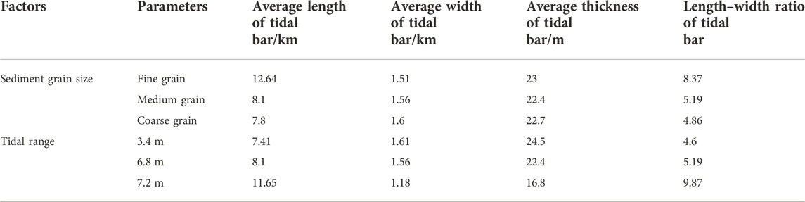
TABLE 1. Quantitative comparison of sand bar shapes under various factors in tidal-controlled estuaries.
Based on the three sets of simulation results with different tidal ranges, we found that when the tidal range is 7.2m, the length-to-width ratio of the sand bar is 9.87 and that the tidal range of 7.2 m has the greatest impact on the development of sediments in tidal-controlled estuaries. Under the simulated conditions of a tidal range of 7.2m, the sand bars have a high degree of development, the length increases with the height of the tidal range, and a long-strip sand bar is developed. The simulation results are similar to those determined in the works of Lageweg et al. (2018) and Leuven et al. (2016). In this study, the tidal channel that developed in the tidal-controlled estuary was complex; the tidal intensity was stronger; the tidal channel was stronger; there were more sand bars; and the shape of the estuary was more complex. In tidal-controlled estuaries, tides play a major role in the shape of the estuary. The greater the tidal range, the higher the degree of estuary development.
Based on the analysis of the main factors controlling sand bar development in tidal-controlled estuaries, the influence of the tidal range and sediment grain size on the shale layer is further studied.
Figures 3, 4 are distribution diagrams of the thickness and length of the muddy shale layer at three tidal heights. According to the thickness distribution diagram in Figure 4, the thickness of most (61%) shale layers is concentrated at 0.1 m, and the thickness of most (87%) shale layers is concentrated between 0.04 m and 0.2 m. According to the distribution of shale layer length, 30% of the shale layer length is concentrated in the range of 0.5 km–2.5 km, and 70% of the shale layer length is greater than 8 km. When the tidal range is 3.4 m, the thickness is concentrated at 0.265 m, and the length is concentrated at 0.5 km and 2.5 km; when the tide is 6.8 m, the shale layer thickness is concentrated at 0.1 m and 0.15 m, and the length is concentrated at 1.8 m, 9.5 km, and 11 km. When the tide is 7.2 m, the thickness of the shale layer is concentrated at 0.07 m and 0.2 m, and the length is concentrated at 8.5 km and 10.5 km. Table 2 gives out the quantitative comparison of shale interlayer in the tidal bars under various tidal ranges. It can be seen from the above that the greater the tide range, the thinner the thickness of the shale layer, and the longer the length of the shale layer.
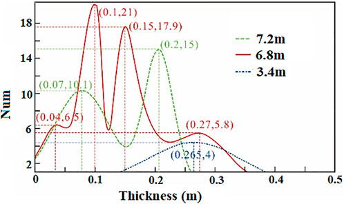
FIGURE 3. Thickness distribution inside the tidal shale layer.
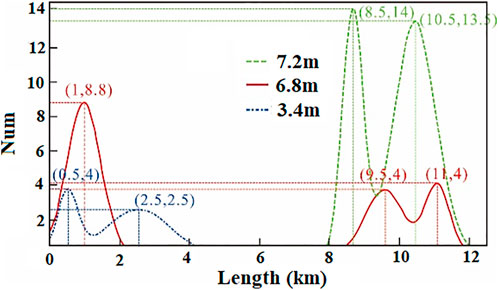
FIGURE 4. Extension length distribution inside shale layer.
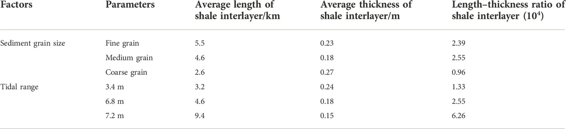
TABLE 2. Quantitative comparison of shale interlayer shapes in tidal bars under various factors in tidal-controlled estuaries.
Figure 5 and Figure 6 show the distribution frequency of the thickness and length of the shale layer in the tidal bars under the three different sediment grain size simulation scenarios. When the grain size of the sediments is fine, the thickness of the shale layer is mainly between 0.1 m-0.45 m and 0.75 m–1 m, and the length is mainly between 1 km and 6 km; when the grain size of the sediments is medium, the shale layer thickness is mainly between 0.05 m and 0.35 m, and the length is mainly between 0–2 km and 8 km–11 km; when the grain size of the sediments is large, the shale layer thickness is mainly between 0.1 m and 0.3 m, and the length is mainly between 0 km and 4 km. Table 2 gives out the quantitative comparison of shale interlayer in the tidal bars under different sediment grain size. When the grain size is fine, the shale layer is thick and long, and when the grain size is coarse, the shale layer is thin and short. The grain size is inversely proportional to the thickness and length of the shale layer.
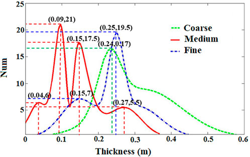
FIGURE 5. Shale layer thickness distribution for different sediment grain sizes.
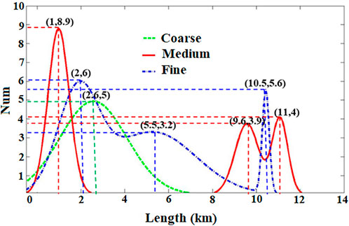
FIGURE 6. Shale layer extension length distribution for different sediment grain sizes.
The sedimentary distribution characteristics of tidal-controlled estuary sand bars are of great significance to the development of sedimentary reservoirs in the tidal-controlled estuaries in the Napo Formation of the Oriente Basin. Based on the Navier–Stokes equation, this study established a dynamic model of tidal-controlled estuary sedimentation, and based on this model, we carried out a numerical simulation of tidal-controlled estuary sand bar sedimentation. The simulation results show that in tidal-controlled estuary environments, both tidal range and sediment grain size have an important influence on the shape of estuary sand bars. The main effect of tidal range on sand bars is that the greater the tidal range, the greater the length-to-width ratio of the sand bars in the estuary, and the higher the degree of sand bar development. When the sediment grain size is fine, more mature sand bars develop, and there is richer variety in the sand bar shapes. Fine-grained sediment could protect the development of estuary sand bars, while a coarser sediment grain size resulted in larger estuary sand bars barely being deposited: they developed slowly in the estuary bay, and there was no sediment deposition in the middle of the estuary. Further comparisons of the influence of the three factors on the morphological parameters of tidal sand bars show that the influence of tidal range on the sedimentary characteristics of tidal sand bars is greater than sediment grain size. Based on the analysis of the main factors controlling sand bar development, the formation and distribution characteristics of shale layers under the environmental conditions of tidal-controlled estuaries were further analyzed. The results show that the length of the shale layer increases as the main controlling factors of the estuary’s tidal range increase, but the changes in thickness are not obvious. The estuary sediment dynamics simulation method proposed in this study can provide model guidance for the exploration and development of estuary sand body sedimentary reservoirs in future research.
The raw data supporting the conclusions of this article will be made available by the authors, without undue reservation.
CZ organized and written the article, YH,SW, MT, KZ, HC, XW, WH, DH, and ZM provided supporting data. all authors agree to be accountable for the content of the work.
This research was funded by the National Natural Science Foundation (grant numbers 42072163,12104513, and 21776315) and the Natural Science Foundation of Shandong Province (grant number ZR2019MD006).
XW was employed by Andes Petroleum Ecuador Ltd.
The remaining authors declare that the research was conducted in the absence of any commercial or financial relationships that could be construed as a potential conflict of interest.
All claims expressed in this article are solely those of the authors and do not necessarily represent those of their affiliated organizations, or those of the publisher, the editors and the reviewers. Any product that may be evaluated in this article, or claim that may be made by its manufacturer, is not guaranteed or endorsed by the publisher.
Alam, R. (2014). Characteristics of hydrodynamic processes in the meghna estuary due to dynamic whirl action. IOSR J. Eng. 4, 39–50. doi:10.9790/3021-04633950
Billy, J., Chaumillon, E., Fenies, H., and Poirier, C. (2012). Tidal and fluvial controls on the morphological evolution of a lobate estuarine tidal bar: The Plassac Tidal Bar in the Gironde Estuary (France). Geomorphology 169-170, 86–97. doi:10.1016/j.geomorph.2012.04.015
Caldwell, R. L., and Edmonds, D. A. (2014). The effects of sediment properties on deltaic processes and morphologies: A numerical modeling study. J. Geophys. Res. Earth Surf. 119, 961–982. doi:10.1002/2013jf002965
Dalrymple, R. W., and Choi, K. (2007). Morphologic and facies trends through the fluvial–marine transition in tide-dominated depositional systems: A schematic framework for environmental and sequence-stratigraphic interpretation. Earth. Sci. Rev. 81, 135–174. doi:10.1016/j.earscirev.2006.10.002
Dalrymple, R., Zaitlin, B., and Boyd, R. (1992). Estuarine faceis models: Conceptual basis and stratigraphic implications. J. Sediment. Res. 62, 1130–1146. doi:10.1306/d4267a69-2b26-11d7-8648000102c1865d
Fairbridge, R. W. (1980). The estuary: Its definition and geodynamic cycle. Chem. Biogeochem. Estuaries 1, 1–36.
Fan, D., Shang, S., and Cai, G. (2014). Characteristics of tidal-bore deposits and facies associations in the qiantang estuary, China. Mar. Geol. 348, 1–14. doi:10.1016/j.margeo.2013.11.012
Grasso, F., Bismuth, E., and Verney, R. (2021). Unraveling the impacts of meteorological and anthropogenic changes on sediment fluxes along an estuary sea continuum. Sci. Rep. 11, 20230. doi:10.1038/s41598-021-99502-7
Jaillard, E., Bengtson, P., and Dhondt, A. (2006). Late cretaceous marine transgressions in Ecuador and northern Peru: A refined stratigraphic framework. J. S. Am. Earth Sci. 19 (3), 307–323. doi:10.1016/j.jsames.2005.01.006
Lageweg, V., Braat, L., Parsons, D. R., and Kleinhans, M. G. (2018). Controls on mud distribution and architecture along the fluvial-to-marineTransition. Geology 46 (11), 971–974. doi:10.1130/G45504.1
Lageweg, W., and Feldman, H. (2018). Process-based modelling of morphodynamics and bar architecture in confined basins with fluvial and tidal currents. Mar. Geol. 398, 35–47. doi:10.1016/j.margeo.2018.01.002
Leuven, J., Klenhans, M., Weisscher, S., and van der Vegt, M. (2016). Tidal sand bar dimensions and shapes in estuaries. Earth-Science Rev. 161, 204–223. doi:10.1016/j.earscirev.2016.08.004
Ma, Z. Z., Tian, Z. J., Zhou, Y. B., Yang, X. F., and Tian, Y. (2020). Geochemical characterization and origin of crude oils in the Oriente basin, Ecuador, South America. J. S. Am. Earth Sci. 104, 102790. doi:10.1016/j.jsames.2020.102790
Poppeschi, C., Charria, G., Goberville, E., Maury, P. R., Barrier, N., Petton, S., et al. (2021). Unraveling salinity extreme events in coastal environments: A winter focus on the bay of brest. Front. Mar. Sci. 8, 705403. doi:10.3389/fmars.2021.705403
Reisinger, A., Gibeaut, J. C., and Tissot, P. E. (2017). Estuarine suspended sediment dynamics: Observations derived from over a decade of satellite data. Front. Mar. Sci. 4, 233. doi:10.3389/fmars.2017.00233
Schramkowski, G., Schuttelaars, H., and de Swart, H. (2002). The effect of geometry and bottom friction on local bed forms in a tidal embayment. Cont. Shelf Res. 22 (11-13), 1821–1833. doi:10.1016/S0278-4343(02)00040-7
Tang, M., Lu, S., Zhang, K., Yin, X., Ma, H., Shi, X., et al. (2019). A three dimensional high-resolution reservoir model of Napo Formation in Oriente Basin, Ecuador, integrating sediment dynamic simulation and geostatistics. Mar. Petroleum Geol. 110, 240–253. doi:10.1016/j.marpetgeo.2019.07.022
Toffolon, M., and Crosato, A. (2007). Developing macroscale indicators for estuarine morphology: The case of the scheldt estuary. J. Coast. Res. 231, 195–212. doi:10.2112/03-0133.1
Van, D. L., and Feldman, H. (2018). Process-based modelling of morphodynamics and bar architecture in confined basins with fluvial and tidal currents. Mar. Geol. 398, 35–47. doi:10.1016/j.margeo.2018.01.002
Weisscher, S., Shimizu, Y., and Kleinhans, M. G. (2019). Upstream perturbation and floodplain formation effects on chute-cutoff-dominated meandering river pattern and dynamics. Earth Surf. Process. Landf. 44 (11), 2156–2169. doi:10.1002/esp.4638
Xie, D., Pan, C., Gao, S., and Wang, Z. (2018). Morphodynamics of the Qiantang Estuary, China: Controls of river flood events and tidal bores. Mar. Geol. 406, 27–33. doi:10.1016/j.margeo.2018.09.003
Yang, X., Ma, Z., Zhou, Y., Zhang, Z., Liu, Y., Wang, D., et al. (2018). Reservoir characteristics and hydrocarbon accumulation of the glauconitic sandstone in the Tarapoa Block, Oriente Basin, Ecuador. J. Petroleum Sci. Eng. 173, 558–568. doi:10.1016/j.petrol.2018.10.059
Zhang, H., Shi, J., and Li, X. (2018). Optimization of shale gas reservoir evaluation and assessment of shale gas resources in the Oriente Basin in Ecuador. Pet. Sci. 15 (4), 756–771. doi:10.1007/s12182-018-0273-7
Keywords: tide sand bar, sediment dynamic simulation, estuary, tidal range, sediment grain size
Citation: Zhang C, Hu Y, Wu S, Tang M, Zhang K, Chen H, Wan X, Huang W, Han D and Meng Z (2023) Analysis of fine grained sand and shale sedimentary characteristics in estuary based on sediment dynamics. Front. Earth Sci. 10:963290. doi: 10.3389/feart.2022.963290
Received: 07 June 2022; Accepted: 19 August 2022;
Published: 05 January 2023.
Edited by:
Kun Zhang, Southwest Petroleum University, ChinaReviewed by:
Yanming Huang, Yangtze University, ChinaCopyright © 2023 Zhang, Hu, Wu, Tang, Zhang, Chen, Wan, Huang, Han and Meng. This is an open-access article distributed under the terms of the Creative Commons Attribution License (CC BY). The use, distribution or reproduction in other forums is permitted, provided the original author(s) and the copyright owner(s) are credited and that the original publication in this journal is cited, in accordance with accepted academic practice. No use, distribution or reproduction is permitted which does not comply with these terms.
*Correspondence: Mingming Tang, dGFuZ21pZ25taW5nMTI2QDEyNi5jb20=
†These authors have contributed equally to this work and share first authorship
Disclaimer: All claims expressed in this article are solely those of the authors and do not necessarily represent those of their affiliated organizations, or those of the publisher, the editors and the reviewers. Any product that may be evaluated in this article or claim that may be made by its manufacturer is not guaranteed or endorsed by the publisher.
Research integrity at Frontiers
Learn more about the work of our research integrity team to safeguard the quality of each article we publish.