The connection of velocity and impedance sensitivity kernels with scattering-angle filtering and its application in full waveform inversion

Multi-scale strategies such as starting from the low-frequency and early-arrival part of recorded data are commonly used in full waveform inversion (FWI) to maneuver complex nonlinearity. An alternative way is to apply appropriate filtering and conditioning to the misfit gradient in the model domain. In acoustic constant-density media, we prove that velocity and impedance sensitivity kernels are equivalent to applying a high-pass and a low-pass scattering-angle filter to a conventional single-parameter velocity (CSV) kernel. The high-pass scattering-angle filter allows the velocity kernel to include low-wavenumber updates (tomography component). In contrast, the low-pass scattering-angle filter helps the impedance kernel to yield high-wavenumber updates (migration component). The velocity model can be updated using a hybrid gradient of two components combined with appropriate weights. This FWI scheme is able to overcome the potential nonlinearity and partially mitigate the cycle-skipping problem. Numerical examples for the SEG/EAGE overthrust model and the Marmousi model demonstrate that the hybrid gradient facilitates FWI to converge faster to the true model even in cases when conventional CSV-based FWI fails.

1 Introduction

Full waveform inversion (FWI) aims to estimate subsurface rock parameters by minimizing misfits between observed and synthetic data (Lailly, 1983; Tarantola, 1984; Mora, 1989; Pratt et al., 1998; Pratt, 1999; Pratt and Shipp, 1999). To date, global optimization methods are still expensive in practice due to high computational costs for forward calculations and high dimensionality of model space. Gradient-based local optimization techniques are commonly used to update model parameters (Tromp et al., 2005; Liu and Tromp, 2006; Plessix, 2006). Due to irregular acquisition, limited offset, ambient noise and lack of low-frequency signals, the nonlinearity of FWI becomes much complicated and the gradient-based solvers are prone to be trapped in the local minima (Brossier et al., 2009; Virieux and Operto, 2009; Sears et al., 2010; Vigh et al., 2010).

Multi-scale strategy is a natural way to reduce the potential nonlinearity through data decimation and selection, which helps FWI to mitigate the cycle-skipping problems (Bunks et al., 1995; Pratt et al., 1996; Virieux and Operto, 2009). One implementation of this strategy is to gradually increase frequency bands to ensure that the phase difference between the predicted and observed data is always less than half a period (Pratt, 1999; Ravaut et al., 2004; Sirgue and Pratt, 2004; Brossier et al., 2009; Fichtner et al., 2013; Xue et al., 2016). The success of this approach requires the existence of effective low-frequency signals in the recorded data, which can be achieved by either acquiring broadband data or utilizing low-frequency enhanced techniques (Xie, 2013; Li and Demanet, 2016; Wang and Herrmann, 2016). Another implementation of multi-scale strategy is to gradually include later arrivals by designing particular windows in the time domain (Shipp and Singh, 2002; Sheng et al., 2006; Brossier et al., 2009; Boonyasiriwat et al., 2010) or introducing proper damping terms in the frequency domain (Shin et al., 2002; Brenders and Pratt, 2007; Shin and Cha, 2008). In addition, layer-stripping and offset-dependent windowing can also be combined with the above two strategies to reduce the nonlinearity and improve the success probability of FWI (Shipp and Singh, 2002; Brossier et al., 2009; Virieux and Operto, 2009).

As analyzed by Wu and Toksöz (1987) and Mora (1989), the resolved wavenumbers of velocity model are determined by scattering patterns in diffraction tomography. Such works provide insights in the model domain instead of the data domain, such as filtering and conditioning the misfit gradient, to reduce the potential nonlinearity in FWI (Albertin et al., 2013; Almomin and Biondi, 2013; Tang et al., 2013; Alkhalifah, 2016). Using the slopes of subsurface structures, Guitton et al. (2012) and Ma et al. (2012) design a directional smoothing operator for the gradients, which can help them to generate smooth velocity models and mitigate the cycle-skipping problem. Tang et al. (2013) notice that the FWI gradient includes tomography and migration components. They propose to enhance the tomography part at early stages in order to recover long-wavelength velocity perturbations. From the standpoint of wavenumber continuation, Alkhalifah (2015) design a scattering-angle filter to extract different wavenumber components and prove that even 10 Hz data can produce vertical near-zero wavenumber components in the FWI gradients. This allows him to update the velocity model from low-to high-wavenumbers by successively relaxing the scattering-angle filter (Wu and Alkhalifah, 2015; Alkhalifah, 2016; Kazei et al., 2016). Wu and Alkhalifah (2017) split the velocity model into background and perturbation components, integrate them directly in the wave equation and introduce a new cheap implementation of scattering angle enrichment, achieving the separation of the background and perturbation components efficiently (Wu and Alkhalifah, 2017).

In this study, we parameterize the acoustic wave equation with velocity and impedance and derive their sensitivity kernels using the Lagrange multiplier method. For a constant-density model, we analytically prove that the velocity and impedance kernels are equivalent to applying a high-pass and a low-pass scattering-angle filter to the conventional single-parameter velocity (CSV) kernel. The high-pass scattering-angle filter allows the velocity kernel to recover low-wavenumber perturbations (tomography component) and can be used to estimate macro velocity models. The low-pass scattering-angle filter helps the impedance kernel to update high-wavenumber perturbations (migration component) and produces high-resolution results. Similar to Tang et al. (2013), we combine these two components into a hybrid gradient (HG) to update the velocity model. By emphasizing the velocity kernel at a few early iterations and then relaxing its weights at later iterations, HG-based FWI provides us with a way to reduce FWI nonlinearity and partially mitigate the cycle-skipping problem. Numerical examples for the SEG/EAGE overthrust and the Marmousi models demonstrate that the proposed method is much more accurate than CSV-based FWI for recovering deep low-wavenumber velocity anomalies.

This paper is organized as follows. First, we derive the velocity and impedance sensitivity kernels using the Lagrange multiplier method. Next, we establish a connection between the velocity and impedance kernels with scattering-angle filtering. Then, we combine these two kernels into a hybrid gradient by properly choosing weights, and apply it to FWI to recover velocity models. Finally, two synthetic examples are used to illustrate the performance of the proposed method.

2 Theory

2.1 Velocity and impedance sensitivity kernels

Using velocity v(x) and impedance z(x) as model parameters, the second-order acoustic wave equation can be written as (Plessix and Li, 2013)

$\frac{1}{v\left(\mathbf{x}\right)z\left(\mathbf{x}\right)}\frac{{\partial }^{2}p\left(\mathbf{x},t\right)}{\partial t^2}-\nabla \cdot \left(\frac{v\left(\mathbf{x}\right)}{z\left(\mathbf{x}\right)}\nabla p\left(\mathbf{x},t\right)\right)=f\left({\mathbf{x}}_s,t\right),(1)$

where x_s and x are the source and subsurface locations, f (x_s, t) is the source function, p (x, t) is the pressure wavefield, which is subject to the initial conditions: p (x, 0) = 0 and ∂p (x, t)/∂t=0.

To derive the adjoint wave equation and sensitivity kernels, we use the Lagrange multiplier method. The augmented least-squares waveform function can be formulated as (Tromp et al., 2005; Liu and Tromp, 2006; Plessix, 2006)

$\begin{array}{cc}\hfill J& =\frac{1}{2}\sum _{{\mathbf{x}}_r}{\int }_0^T{\left[p\left({\mathbf{x}}_r,t\right)-d\left({\mathbf{x}}_r,t\right)\right]}^{2}dt\hfill \\ \hfill & -{\int }_0^T{\int }_{\mathrm{\Omega }}q\left(\mathbf{x},t\right)\left[\frac{1}{v\left(\mathbf{x}\right)z\left(\mathbf{x}\right)}\frac{{\partial }^{2}p\left(\mathbf{x},t\right)}{\partial t^2}-\nabla \cdot \left(\frac{v\left(\mathbf{x}\right)}{z\left(\mathbf{x}\right)}\nabla p\left(\mathbf{x},t\right)\right)\right]{d\mathbf{x}}^{3}dt,\hfill \end{array}(2)$

where x_r is the receiver location, q (x, t) is the Lagrange multiplier, [0, T] denotes the record duration, Ω is the subsurface volume of interest. Taking the variation of J in Eq. 2 and using integration by parts for the spatial derivatives of p (x, t), we obtain

$\begin{array}{cc}\hfill \delta J& ={\int }_0^T{\int }_{\mathrm{\Omega }}\sum _{{\mathbf{x}}_r}\left[p\left({\mathbf{x}}_r,t\right)-d\left({\mathbf{x}}_r,t\right)\right]\delta p\left(\mathbf{x},t\right)\delta \left(\mathbf{x}-{\mathbf{x}}_r\right){d\mathbf{x}}^{3}dt\hfill \\ \hfill & -{\int }_0^T{\int }_{\mathrm{\Omega }}\left\{\delta p\left(\mathbf{x},t\right)\left[\frac{1}{v\left(\mathbf{x}\right)z\left(\mathbf{x}\right)}\frac{{\partial }^{2}q\left(\mathbf{x},t\right)}{\partial t^2}-\nabla \cdot \left(\frac{v\left(\mathbf{x}\right)}{z\left(\mathbf{x}\right)}\nabla q\left(\mathbf{x},t\right)\right)\right]\right.\hfill \\ \hfill & -\delta \ln v\left[\frac{1}{z\left(\mathbf{x}\right)v\left(\mathbf{x}\right)}\frac{{\partial }^{2}p\left(\mathbf{x},t\right)}{\partial t^2}q\left(\mathbf{x},t\right)-\frac{v\left(\mathbf{x}\right)}{z\left(\mathbf{x}\right)}\nabla p\left(\mathbf{x},t\right)\cdot \nabla q\left(\mathbf{x},t\right)\right]\hfill \\ \hfill & -\left.\delta \ln z\left[\frac{1}{z\left(\mathbf{x}\right)v\left(\mathbf{x}\right)}\frac{{\partial }^{2}p\left(\mathbf{x},t\right)}{\partial t^2}q\left(\mathbf{x},t\right)+\frac{v\left(\mathbf{x}\right)}{z\left(\mathbf{x}\right)}\nabla p\left(\mathbf{x},t\right)\cdot \nabla q\left(\mathbf{x},t\right)\right]\right\}{d\mathbf{x}}^{3}dt,\hfill \end{array}(3)$

where δ(x) is the Dirac delta function, δp (x, t) is the perturbed pressure wavefield. δ ln z = δz(x)/z₀(x), δ ln v = δv(x)/v₀(x), where δz(x) and z₀(x) are the perturbed and background impedances respectively, δv(x) and v₀(x) are the perturbed and background velocities. Note that in (Eq. 3), we only consider the first-order expansion for the pressure wavefield and model parameters, which is known as the Born approximation (Tarantola, 2005; Tromp et al., 2005; Plessix, 2006).

Provided the Lagrange multiplier q (x, t) satisfies

$\frac{1}{v\left(\mathbf{x}\right)z\left(\mathbf{x}\right)}\frac{{\partial }^{2}q\left(\mathbf{x},t\right)}{\partial t^2}-\nabla \cdot \left(\frac{v\left(\mathbf{x}\right)}{z\left(\mathbf{x}\right)}\nabla q\left(\mathbf{x},t\right)\right)=\sum _{{\mathbf{x}}_r}\left[p\left({\mathbf{x}}_r,t\right)-d\left({\mathbf{x}}_r,t\right)\right]\delta \left(\mathbf{x}-{\mathbf{x}}_r\right)(4)$

and is subject to the final conditions

$q\left(\mathbf{x},T\right)=0,\frac{\partial q\left(\mathbf{x},T\right)}{\partial t}=0,(5)$

(Eq. 3) can be simplified to

$\begin{array}{cc}\hfill \delta J& =-{\int }_0^T{\int }_{\mathrm{\Omega }}\left\{\delta \ln v\left[\frac{1}{z\left(\mathbf{x}\right)v\left(\mathbf{x}\right)}\frac{{\partial }^{2}p\left(\mathbf{x},t\right)}{\partial t^2}q\left(\mathbf{x},t\right)-\frac{v\left(\mathbf{x}\right)}{z\left(\mathbf{x}\right)}\nabla p\left(\mathbf{x},t\right)\cdot \nabla q\left(\mathbf{x},t\right)\right]\right.\hfill \\ \hfill & +\left.\delta \ln z\left[\frac{1}{z\left(\mathbf{x}\right)v\left(\mathbf{x}\right)}\frac{{\partial }^{2}p\left(\mathbf{x},t\right)}{\partial t^2}q\left(\mathbf{x},t\right)+\frac{v\left(\mathbf{x}\right)}{z\left(\mathbf{x}\right)}\nabla p\left(\mathbf{x},t\right)\cdot \nabla q\left(\mathbf{x},t\right)\right]\right\}{d\mathbf{x}}^{3}dt.\hfill \end{array}(6)$

This equation tells us that the change of the misfit δJ may be caused by the changes of the model parameters δ ln z and δ ln v in terms of the forward wavefield p (x, t) and the Lagrange multiplier wavefield q (x, t). The adjoint wavefield is defined as p^†(x, t) = q (x, T − t) and inserted into Eq. 4 to obtain the adjoint wave equation

$\frac{1}{v\left(\mathbf{x}\right)z\left(\mathbf{x}\right)}\frac{{\partial }^2{p}^{†}\left(\mathbf{x},t\right)}{\partial t^2}-\nabla \cdot \left(\frac{v\left(\mathbf{x}\right)}{z\left(\mathbf{x}\right)}\nabla p^{†}\left(\mathbf{x},t\right)\right)=\sum _{{\mathbf{x}}_r}\left[p\left({\mathbf{x}}_r,T-t\right)-d\left({\mathbf{x}}_r,T-t\right)\right]\delta \left(\mathbf{x}-{\mathbf{x}}_r\right).(7)$

Then, the variation of the misfit function in (Eq. 6) is reduced to

$\begin{array}{c}\hfill \delta J=-{\int }_{\mathrm{\Omega }}\left(\delta \ln v{K}_v+\delta \ln z{K}_z\right){d\mathbf{x}}^3.\end{array}(8)$

where the velocity (K_v) and impedance (K_z) kernels are defined as

$\begin{array}{cc}\hfill K_v\left(\mathbf{x}\right)& ={\int }_0^T\left[\frac{1}{z\left(\mathbf{x}\right)v\left(\mathbf{x}\right)}\frac{{\partial }^{2}p\left(\mathbf{x},t\right)}{\partial t^2}{p}^{†}\left(\mathbf{x},T-t\right)-\frac{v\left(\mathbf{x}\right)}{z\left(\mathbf{x}\right)}\nabla p\left(\mathbf{x},t\right)\cdot \nabla p^{†}\left(\mathbf{x},T-t\right)\right]dt,\hfill \\ \hfill K_z\left(\mathbf{x}\right)& ={\int }_0^T\left[\frac{1}{z\left(\mathbf{x}\right)v\left(\mathbf{x}\right)}\frac{{\partial }^{2}p\left(\mathbf{x},t\right)}{\partial t^2}{p}^{†}\left(\mathbf{x},T-t\right)+\frac{v\left(\mathbf{x}\right)}{z\left(\mathbf{x}\right)}\nabla p\left(\mathbf{x},t\right)\cdot \nabla p^{†}\left(\mathbf{x},T-t\right)\right]dt.\hfill \end{array}(9)$

Note that the adjoint wave equation is exactly the same as the forward wave (Eq. 1), except for replacing f (x_s, t) by time-reversed data residual (adjoint source).

For comparison, herein present the CSV kernel (the detailed derivation is given in Appendix A):

$K_{\mathit{csv}}\left(\mathbf{x}\right)=2{\int }_0^T\left[\frac{1}{z\left(\mathbf{x}\right)v\left(\mathbf{x}\right)}\frac{{\partial }^{2}p\left(\mathbf{x},t\right)}{\partial t^2}{p}^{†}\left(\mathbf{x},T-t\right)\right]dt.(10)$

(Eqs. 9, 10) show that the CSV kernel equal the summation of the velocity and impedance kernels, indicating that the updates in CSV-based FWI include both velocity and impedance information. Zhou et al. (2015) show that due to the different responses to the scattering angles, the velocity and impedance kernels produce low-wavenumber (tomography) and high-wavenumber (migration) components, respectively (Wu and Toksöz, 1987; Mora, 1989; Alkhalifah, 2015). Therefore, conventional CSV-based FWI simultaneously update the macro and detail structures in velocity model building, which increases the nonlinearity and is prone to be trapped into local minima. One way to mitigate this problem in the model domain is to use the wavenumber continuation strategy that combines the two separated components with proper weights (Tang et al., 2013; Alkhalifah, 2016).

2.3 Connection between velocity and impedance kernels with scattering-angle filtering in constant-density media

Douma et al. (2010) prove that the impedance kernel in adjoint tomography is equivalent to the application of Laplacian filtering to reverse-time migration (RTM) images. Zhang and Sun (2009) notice that the application of the Laplacian filtering to RTM images is equivalent to the application of a cos²ϕ filter to angle-domain gathers, where ϕ is the reflection angle. Such conclusions confirm that the impedance-based imaging condition produces fewer low-wavenumber artifacts on RTM images (Zhu et al., 2009; Whitmore and Crawley, 2012; Pestana et al., 2014). In this section, we extend Douma et al. (2010)’s derivation to both velocity and impedance kernels and establish a connection between these kernels with scattering-angle filtering.

Considering the initial and final conditions for the forward and adjoint wavefields

$p\left(\mathbf{x},0\right)=p^{†}\left(\mathbf{x},T\right)=0,p\left(\mathbf{x},T\right)=p^{†}\left(\mathbf{x},0\right)=0,(11)$

and using integration by parts for the time derivatives, we have the following identity

$\begin{array}{cc}\hfill {\int }_0^T\left[\frac{{\partial }^{2}p\left(\mathbf{x},t\right)}{\partial t^2}{p}^{†}\left(\mathbf{x},T-t\right)\right]dt& =-{\int }_0^T\left[\frac{\partial p\left(\mathbf{x},t\right)}{\partial t}\frac{d{p}^{†}\left(\mathbf{x},T-t\right)}{dt}\right]dt\hfill \\ \hfill & ={\int }_0^T\left[p\left(\mathbf{x},t\right)\frac{{\partial }^2{p}^{†}\left(\mathbf{x},T-t\right)}{\partial t^2}\right]dt.\hfill \end{array}(12)$

This notation simplifies the velocity and impedance kernels in (Eq. 9) to

$\begin{array}{cc}\hfill K_v\left(\mathbf{x}\right)& =\frac{1}{2}\frac{v\left(\mathbf{x}\right)}{z\left(\mathbf{x}\right)}{\int }_0^T\left[\frac{1}{v^2\left(\mathbf{x}\right)}\frac{{\partial }^{2}p\left(\mathbf{x},t\right)}{\partial t^2}{p}^{†}\left(\mathbf{x},T-t\right)\right.\hfill \\ \hfill & -\left.2\nabla p\left(\mathbf{x},t\right)\cdot \nabla p^{†}\left(\mathbf{x},T-t\right)+\frac{1}{v^2\left(\mathbf{x}\right)}p\left(\mathbf{x},t\right)\frac{{\partial }^2{p}^{†}\left(\mathbf{x},T-t\right)}{{\partial }^{2}t}\right]dt,\hfill \\ \hfill K_z\left(\mathbf{x}\right)& =\frac{1}{2}\frac{v\left(\mathbf{x}\right)}{z\left(\mathbf{x}\right)}{\int }_0^T\left[\frac{1}{v^2\left(\mathbf{x}\right)}\frac{{\partial }^{2}p\left(\mathbf{x},t\right)}{\partial t^2}{p}^{†}\left(\mathbf{x},T-t\right)\right.\hfill \\ \hfill & +\left.2\nabla p\left(\mathbf{x},t\right)\cdot \nabla p^{†}\left(\mathbf{x},T-t\right)+\frac{1}{v^2\left(\mathbf{x}\right)}p\left(\mathbf{x},t\right)\frac{{\partial }^2{p}^{†}\left(\mathbf{x},T-t\right)}{{\partial }^{2}t}\right]dt.\hfill \end{array}(13)$

In isotropic acoustic media with constant density, i.e., z(x)/v(x) = ρ₀, the forward and adjoint wavefields satisfy

$\begin{array}{c}\hfill \frac{1}{v^2\left(\mathbf{x}\right)}\frac{{\partial }^{2}p\left(\mathbf{x},t\right)}{\partial t^2}-{\nabla }^{2}p\left(\mathbf{x},t\right)={\rho }_{0}f\left({\mathbf{x}}_s\right),\frac{1}{v^2\left(\mathbf{x}\right)}\frac{{\partial }^2{p}^{†}\left(\mathbf{x},t\right)}{\partial t^2}-{\nabla }^2{p}^{†}\left(\mathbf{x},t\right)={\rho }_0{f}^{†}\left(\mathbf{x},t\right),\end{array}(14)$

where f^†(x, t) is the adjoint source, that is, the right-hand side of (Eq 7). Inserting (Eq. 14) into (Eq. 13) and replacing the time-derivatives with the spatial-derivatives of p (x, t) and p^†(x, t) yields

$\begin{array}{cc}\hfill K_v\left(\mathbf{x}\right)& =\frac{1}{2{\rho }_0}{\int }_0^T\left[{\nabla }^{2}p\left(\mathbf{x},t\right)p^{†}\left(\mathbf{x},T-t\right)-2\nabla p\left(\mathbf{x},t\right)\cdot \nabla p^{†}\left(\mathbf{x},T-t\right)\right.\hfill \\ \hfill & +\left.p\left(\mathbf{x},t\right){\nabla }^2{p}^{†}\left(\mathbf{x},T-t\right)\right]dt,\hfill \\ \hfill K_z\left(\mathbf{x}\right)& =\frac{1}{2{\rho }_0}{\int }_0^T\left[{\nabla }^{2}p\left(\mathbf{x},t\right)p^{†}\left(\mathbf{x},T-t\right)+2\nabla p\left(\mathbf{x},t\right)\cdot \nabla p^{†}\left(\mathbf{x},T-t\right)\right.\hfill \\ \hfill & +\left.p\left(\mathbf{x},t\right){\nabla }^2{p}^{†}\left(\mathbf{x},T-t\right)\right]dt.\hfill \end{array}(15)$

In (Eq. 15), the terms associated with the source and the adjoint source are neglected because they vanish for far-field wavefields (Douma et al., 2010). Applying Fourier transform to (Eq. 15) and because $\left|\mathbf{k}\right|=\left|{\mathbf{k}}^{†}\right|=\omega /v$, the kernels have the following form:

$\begin{array}{cc}\hfill K_v\left(\mathbf{k}\right)& =\frac{1}{{\rho }_0}\sum _{\omega }|\mathbf{k}{|}^2\left(1-\frac{\mathbf{k}\cdot {\mathbf{k}}^{†}}{|\mathbf{k}{|}^2}\right)P\left(\mathbf{k},\omega \right)P^{†}\left(\mathbf{k},\omega \right),\hfill \\ \hfill K_z\left(\mathbf{k}\right)& =\frac{1}{{\rho }_0}\sum _{\omega }|\mathbf{k}{|}^2\left(1+\frac{\mathbf{k}\cdot {\mathbf{k}}^{†}}{|\mathbf{k}{|}^2}\right)P\left(\mathbf{k},\omega \right)P^{†}\left(\mathbf{k},\omega \right).\hfill \end{array}(16)$

where ω is the angular frequency, p (k, ω) and p^†(k, ω) are the forward and adjoint Fourier-domain wavefields, k and k^† are the forward and adjoint wavenumbers. Considering the relation $\frac{\mathbf{k}\cdot {\mathbf{k}}^{†}}{|\mathbf{k}{|}^2}=\cos \theta$ and using the dispersion relation |k|² = ω²/v², (Eq. 16) can be reformulated as

$\begin{array}{cc}\hfill K_v\left(\mathbf{x}\right)& =\frac{2}{{\rho }_0}\sum _{\omega }\frac{{\omega }^2}{v^2\left(\mathbf{x}\right)}P\left(\mathbf{x},\omega \right)P^{†}\left(\mathbf{x},\omega \right)\frac{\left(1-\cos \theta \right)}{2},\hfill \\ \hfill K_z\left(\mathbf{x}\right)& =\frac{2}{{\rho }_0}\sum _{\omega }\frac{{\omega }^2}{v^2\left(\mathbf{x}\right)}P\left(\mathbf{x},\omega \right)P^{†}\left(\mathbf{x},\omega \right)\frac{\left(1+\cos \theta \right)}{2}.\hfill \end{array}(17)$

where θ is the scattering angle (see Figure 1). Similarly, CSV kernel in (Eq. 10) can be rewritten in the frequency domain as

$\begin{array}{c}\hfill K_{\mathit{csv}}\left(\mathbf{x}\right)=\frac{2}{{\rho }_0}\sum _{\omega }\frac{{\omega }^2}{v^2\left(\mathbf{x}\right)}P\left(\mathbf{x},\omega \right)P^{†}\left(\mathbf{x},\omega \right).\end{array}(18)$

(Eqs. 17, 18) show that the differences between K_v and K_z with K_csv are the multiplication with (1 − cos θ)/2 and (1 + cos θ)/2, which appear as band-pass filters associated with scattering angles. Note that K_z includes both velocity and density updates when density varies significantly in the subsurface. Since (Eqs. 12–17) are derived based on the assumption of constant density, K_z and K_v herein represent the velocity perturbations within different scattering-angle bands.

FIGURE 1

FIGURE 1. Geometry of incident and scattering waves. Red lines are the wave paths of the forward and adjoint wavefields. k and k^† denote their propagation directions. (x, z) is the Cartesian coordinate system and θ is the scattering angle.

A simple experiment (Figure 2) is used to illustrate the effects of these two scattering-angle filters. Since the sensitivity kernels in (Eqs. 17, 18) are derived based on Born approximation, we calculate Born modeling results using CSV parameterization as well as velocity and impedance parameterization (Figures 2B–D). These results are also known as radiation patterns (Virieux and Operto, 2009; Wang et al., 2015; Zhou et al., 2015). Figure 2A shows that the CSV kernel has an all-pass response with respect to scattering angles, which corresponds to a homogenous radiation pattern (Figure 2B). This suggests that the CSV kernel includes both large and small scattering-angle updates (Tang et al., 2013). The velocity kernel K_v behaves like applying a high-pass filter to the CVS kernel (red line in Figure 2A), which emphasizes large-angle forward scattering contributions (Figure 2C). This indicates that the tomography component in FWI gradient is enhanced in K_v and can be used to recover large- and intermediate-scale velocity perturbations. In contrast, the impedance kernel K_z is a result of applying a low-pass scattering-angle filter to the CSV kernel (green line in Figure 2A), emphasizing the small-angle backscattering component (Figure 2D). This high-pass scattering-angle filter helps us to produce migration profiles and can be used to resolve detail structures (Luo et al., 2009; Zhu et al., 2009; Pestana et al., 2014).

FIGURE 2

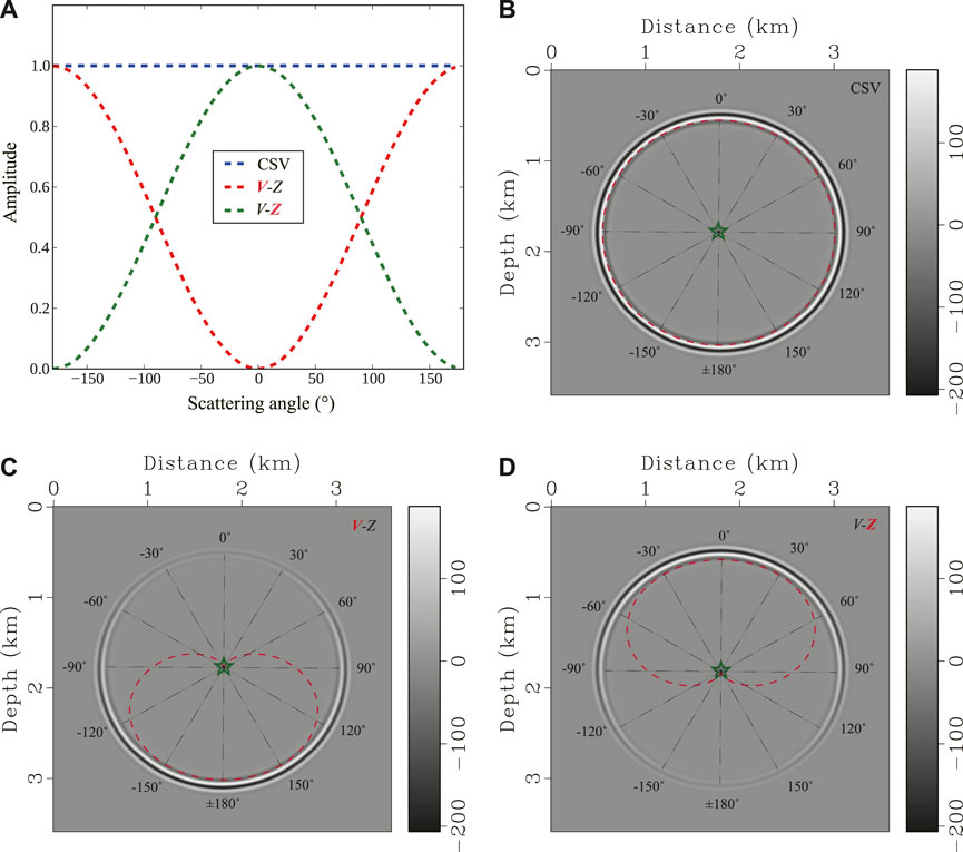
FIGURE 2. Scattering angle filters and radiation patterns for a vertically incident plane wave in a homogenous medium with v =2 km/s (A) Angle filters for different kernels; (B) CSV radiation pattern; (C) velocity and (D) impedance radiation patterns. A unit model perturbation indicated by a green star is located at x =2 km and z =2 km. Red dashed lines in (B), (C) and (D) denote the amplitude variations with respect to different scattering angles.

2.4 Full waveform inversion with a hybrid gradient

In the CSV-based FWI, the velocity model can be updated using the following gradient-based scheme:

${\mathbf{m}}^{k+1}={\mathbf{m}}^k-\alpha {\mathbf{H}}^{-1}{\mathbf{g}}^k(19)$

where m^k+1 and m^k are the velocity models in the next and current iterations, respectively; g^k is the misfit gradient, which can be computed by summing K_csv in (Eq. 10) over sources; α is the step length, which can be computed with a line-search algorithm (Potra and Shi, 1995); H⁻¹ is the Hessian inverse and can be used to speed up convergence (Pratt et al., 1998; Shin et al., 2001; Plessix and Mulder, 2004; Tang, 2009; Métivier et al., 2013).

Using wavefield decomposition, Tang et al. (2013) and Wang et al. (2016) show that the enhancement of tomography components in the misfit gradient helps FWI to reduce nonlinearity and mitigate the cycle-skipping problem. This can also be implemented with a wavenumber continuity strategy, designing an appropriate scattering-angle filter (Wu and Alkhalifah, 2015; Alkhalifah, 2016). In the previous section, the connection between the velocity and impedance kernels is established by scattering-angle filtering in acoustic constant-density media. Similar to Tang et al. (2013), we combine the velocity and impedance kernels into a hybrid gradient:

${\mathbf{g}}_h=\lambda \sum _{{\mathbf{x}}_s}{K}_v\left({\mathbf{x}}_s\right)+\sum _{{\mathbf{x}}_s}{K}_z\left({\mathbf{x}}_s\right),(20)$

where x_s is the source location, K_v(x_s) and K_z (x_s) are the kernels in (Eq. 9), and λ is an adjustable scalar parameter to balance the relative weights of K_v and K_z.

Note that the large scattering-angle components in the gradient are enhanced by setting λ greater than one in (Eq. 20) at early iterations, the large scattering-angle components in the gradient are enhanced. This allows us to recover large- and intermediate-scale velocity perturbations. In subsequent iterations, reducing λ gradually to one can increase the relative weight of K_z and use more smaller scattering-angle contributions, which enables us to update detail structures. We refer to this workflow as the HG-based FWI. Since we first update large scattering-angle perturbations and then introduce smaller scatting-angle information, HG-based FWI provides us a possible way to reduce potential nonlinearity during FWI iterations.

3 Numerical examples

We present two synthetic examples to illustrate the performance of the proposed HG-based FWI scheme. The first example is the 2D SEG/EAGE overthrust model, which is modified by adding a 175 m thick water layer on the top of the model. The true velocity model is shown in Figure 3A. Initial model in Figure 3B is built by applying a 625 m × 625 m Gaussian filter to the true model. Seismograms are calculated using a staggered-grid finite-difference scheme with eighth-order accuracy in space and second-order accuracy in time. 25 shots are evenly distributed on the surface with a 250 m interval. Each shot is recorded by 250 receivers, which are uniformly deployed on the surface with a 25 m spacing. A Ricker wavelet with a peak frequency of 20 Hz is used as the source function. A high-pass filter is applied to filter out low-frequency signals below 5 Hz.

FIGURE 3

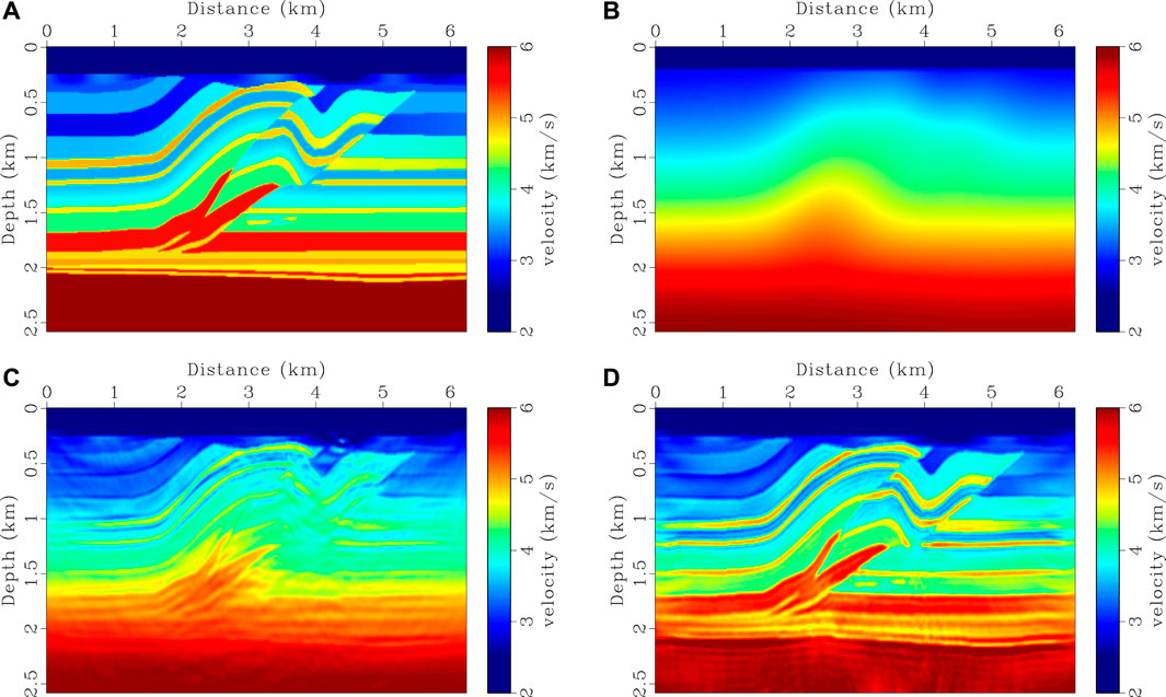
FIGURE 3. FWI experiments for SEG/EAGE overthrust model. (A) True velocity model, (B) initial velocity model, (C) recovered velocity model using CSV-based FWI, and (D) recovered velocity model using HG-based FWI. 40 iterations are performed in (C,D). The lowest effective frequency used in (C,D) is 5 Hz.

Inversion results using CSV-based FWI and our method are shown in Figures 3, 4. 40 iterations are performed and a phase-encoding diagonal Hessian (Figure 6D) is used as a pre-conditioner (Tang, 2009) in both methods. In our method, λ is set to 8.0 in the first 10 iterations, and then gradually reduces to 1.0 during the following iterations as shown in Figure 5. Gradients calculated using different kernels at the first iteration are shown in Figure 6. We notice that the gradient in CSV-based FWI includes almost high-wavenumber updates, i.e., migration components (see Figure 6A). This does not mean there are no low-wavenumber components, but their magnitudes are relatively small in comparison with high-wavenumber components. As shown in Figures 6B,C, the low- and high-pass scattering-angle filters decompose the CSV kernel into a tomography component (K_v) and a migration component (K_z). This favorable scale-separation property allows HG-based FWI to update the low-wavenumber tomography component by enhancing the weight of K_v, and to resolve detail structures by gradually increasing the weight of K_z (see Figures 3D, 4).

FIGURE 4

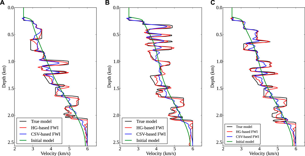
FIGURE 4. Comparisons of velocity logs for SEG/EAGE overthrust model. (A–C) are located at the midpoints of 1.25, 3.5, and 5.0 km, respectively. Black and green lines are from true and initial models, blue and red lines are from CSV-based FWI and HG-based FWI. HG-based FWI produces more accurate results than CSV-based method, especially at great depths with large-scale velocity anomalies.

FIGURE 5

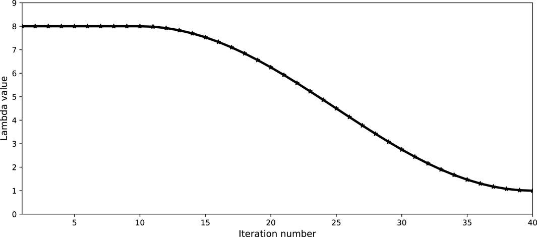
FIGURE 5. The relationship between the weight factor lambda and iterations. λ is set to 8.0 in the first 10 iterations, and then gradually reduces to 1.0 according to the change of cosine function in subsequent iterations.

FIGURE 6

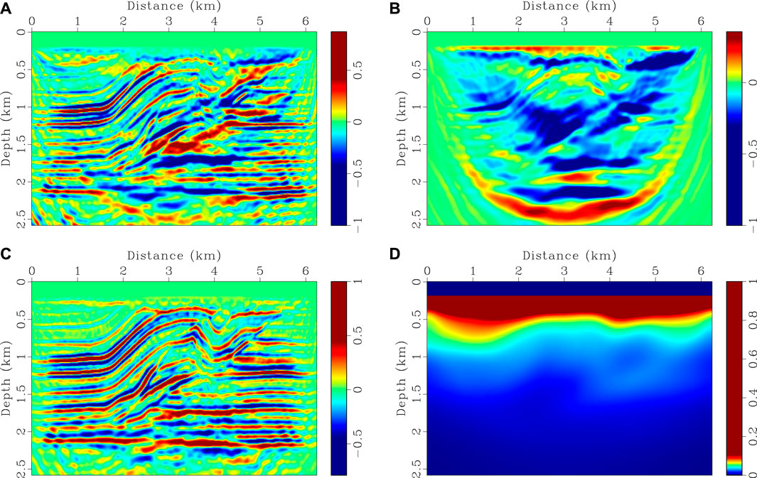
FIGURE 6. Comparison of different gradients in the first iteration for SEG/EAGE overthrust model. (A) CSV-based gradient, (B) velocity and (C) impedance gradients, and (D) phase-encoding diagonal Gauss-Newton Hessian. (D) Is used as a preconditioner in both CSV-based and HG-based FWI methods. The magnitude of each panel is normalized with respect to their maximum values.

Figure 7 shows the evolutions of data residuals and model errors for these two FWI schemes. Data residuals and model errors are defined as

$r=\frac{\Vert {\mathbf{d}}_{\mathit{obs}}-{\mathbf{d}}_{\mathit{syn}}{\Vert }^2}{\Vert {\mathbf{d}}_{\mathit{obs}}{\Vert }^2},e=\frac{\Vert {\mathbf{m}}_{\mathit{tru}}-{\mathbf{m}}_{\mathit{fwi}}{\Vert }^2}{\Vert {\mathbf{m}}_{\mathit{tru}}{\Vert }^2},(21)$

where d_obs and d_syn are the observed and synthetic data, m_tru and m_fwi are the true and recovered velocity models. Relative data residuals and model errors are calculated by normalizing r and e by their initial values (r₀ and e₀). Although the data residual of CSV-based FWI has been reduced by about 90%, it is stuck around 10% (blue line in Figure 7A), suggesting that it is trapped into a local minimum. This is also reflected in the corresponding model errors in Figure 7B. With a hybrid gradient, the proposed method recovers low-wavenumber components first and then gradually increases high-wavenumber components, leading to a faster convergence rate and a higher inversion accuracy in comparison with CSV-based FWI (see Figures 4, 7).

FIGURE 7

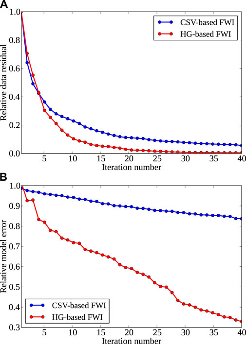
FIGURE 7. Convergence rates for SEG/EAGE overthrust model. (A,B) are relative data residual and model error, respectively. Blue and red lines are results from CSV-based FWI and the proposed HG-based FWI.

In the second example, the Marmousi model is used to test the robustness of the proposed method for complicated structures. True velocity model is shown in Figure 8A. Starting model (Figure 8B) is built by applying a 1,250 m × 1,250 m Gaussian filter to the true model. Seismograms are generated using the same finite-difference scheme as the previous example. Source function is a Ricker wavelet with a peak frequency of 8 Hz. 38 shots are distributed on the surface with a 250 m spacing. 761 receivers are deployed evenly on the model surface with a 12.5 m interval. A dataset is built by filtering frequency components below 3 Hz and is used for both CVS-based FWI and the proposed method. The setting of λ in HG-based FWI is the same as the previous example. Inversion results are shown in Figures 10A,B. Gradients for the first iteration and velocity logs are shown in Figures 9, 11, respectively. CSV-based FWI produces accurate results at shallow depths for both low- and high-wavenumber perturbations, but fails to recover low-wavenumber velocity anomalies at greater depths (see Figures 10A, 11). This is caused by uneven subsurface scattering-angle illuminations. At shallow depths, there is sufficient illumination for both large and small scattering angles due to large offset-to-depth ratio (O/D). As depth increases, O/D decreases and the CSV-based gradient is dominated by small scattering-angle components (Figure 9A). Although large scattering-angle components in deep areas are very weak, they do exist as proved by Alkhalifah (2015). Instead of using the CSV kernel, HG-based FWI combines the K_v and K_z kernels to update velocity model (Figures 9B,C). This helps us to recover low-wavenumber perturbations at greater depths by enhancing the K_v kernel in FWI gradient. Then, high-wavenumber structures are recovered by gradually reducing the weight of the K_v kernel, producing a final high-resolution result (Figures 10B, 11).

FIGURE 8

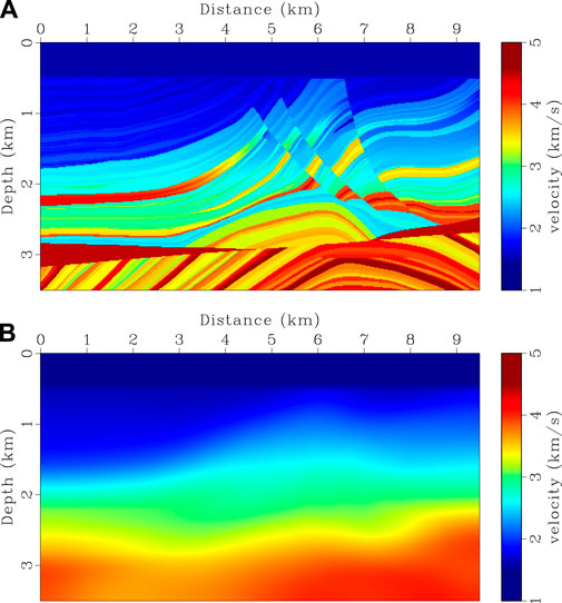
FIGURE 8. FWI experiment for Marmousi model. (A) True velocity model and (B) initial velocity model.

FIGURE 9

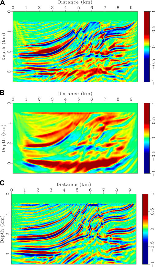
FIGURE 9. Comparisons of different gradients in the first iteration for Marmousi model. (A) CSV-based gradient, (B) velocity and (C) impedance gradients. The magnitude of each panel is normalized with respect to their maximum values.

FIGURE 10

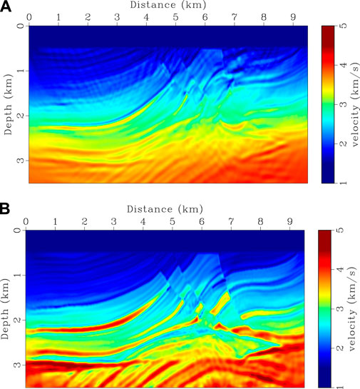
FIGURE 10. Recovered Marmousi velocity model from different FWI methods. (A,B) are CSV-based FWI and our method using data without frequency components below 3 Hz. 40 iterations are used in (A,B).

FIGURE 11

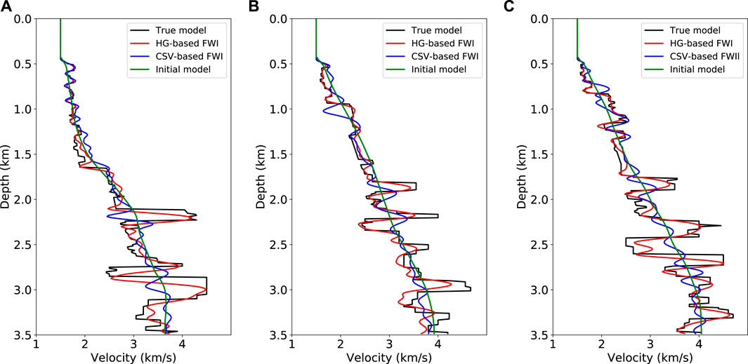
FIGURE 11. Comparisons of velocity logs for Marmousi model. (A–C) are located at the midpoints of 1.8, 5.0, and 8.1 km, respectively. Black and green lines are from true and initial models; blue and red lines are from CSV-based FWI and the proposed method. The proposed method is much more accurate than CSV-based FWI for recovering deep low-wavenumber velocity anomalies.

To better quantitatively evaluate the inversion results of these two methods, we compare their convergence rates (Figure 12) and predicted seismograms using final recovered models (Figure 13). Compared with CSV-based FWI method (red line in Figure 12), the proposed method has a faster convergence rate and a higher inversion accuracy (blue line in Figure 12), which also can illustrate that the proposed method has better adaptability to complex structures.

FIGURE 12

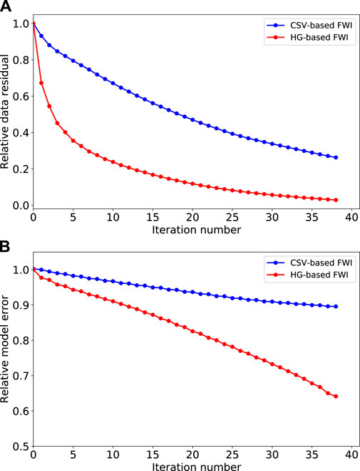
FIGURE 12. Convergence rates for Marmousi model. (A,B) are relative data residual and model error, respectively. Blue and red lines are results from CSV-based FWI and the proposed method.

FIGURE 13

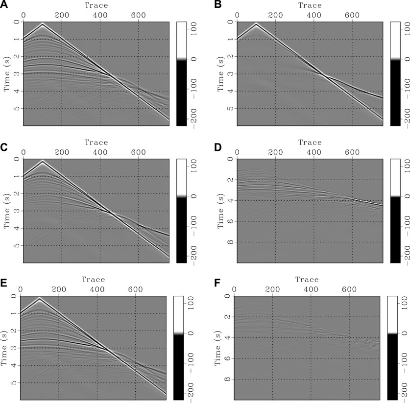
FIGURE 13. Comparisons of common-shot gathers for Marmousi model. (A) Observed data, (B) synthetic data using initial model; (C) synthetic data using CSV-based FWI velocity model, (D) difference between (A) with (C); (E) synthetic data using recovered velocity model from the proposed method, (F) difference between (A,E).

4 Discussion

By parameterizing the acoustic wave equation using velocity and impedance, we derive their sensitivity kernels based on the Lagrange multiplier method. In a constant-density case, we prove that the velocity (K_v) and impedance (K_z) kernels are equivalent to applying a high-pass and a low-pass scattering-angle filters to the CSV (K_csv) kernel. K_v mainly provides low-wavenumber updates and is helpful to recover large-scale anomalies. Although impedance is defined as z = ρv, K_z represents high-wavenumber velocity perturbations in constant-density media and helps us to resolve detail structures. By choosing weights properly, we can enhance K_v contribution in the hybrid gradient at early iterations and then gradually increase K_z contribution in subsequence iterations. This workflow reduces FWI nonlinearity and partially mitigate the cycle-skipping problem.

The proposed HG-based FWI scheme is similar to the tomography-enhanced FWI presented by Tang et al. (2013). But there are several key differences. First, Tang et al. (2013) use wavefield decomposition to extract the tomography and migration components from the CSV-based gradient. There is no clear relation between these two components with the scattering-angle filtering. Second, in areas with complicated structures, cross-correlations between source-side and receiver-side upgoing waves or between source-side and receiver-side downgoing waves might still produce certain migration components. Third, separating upgoing and downgoing waves requires the construction of an analytical wavefield at every time step. This can be implemented by either solving the wave equation twice (Shen and Albertin, 2015) or calculating a complex-valued wave equation (Zhang and Zhang, 2009; Pestana and Revelo, 2017), thus with a higher computational cost. Our approach only needs to modify the gradient calculation with time- and spatial-derivatives and hence no additional computational costs are required.

In our derivation from (Eqs. 12–18), the subsurface density is assumed to be constant. Therefore, our method is applicable for areas without significant density variations. When density varies greatly, we should consider the spatial derivation of 1/ρ in Eq. 14 and cannot obtain an analytic relation between K_v and K_z with K_csv. In this case, K_z includes both velocity and density perturbations (Prieux et al., 2013; Zhou et al., 2015), and thus cannot be combined with K_v to update the velocity model. How to simultaneously invert multi-parameters, such as velocity and density, velocity and impedance or impedance and density, is beyond the scope of this paper and needs further investigation.

5 Conclusion

We establish a connection between the velocity and impedance kernels with scattering angle filtering in acoustic constant-density media. This allows us to combine these two kernels into a HG-based FWI workflow to update the velocity model. By enhancing the velocity kernel contribution at early iterations, which mainly gives tomography updates, the proposed method enables us to recover large- and intermediate-scale velocity anomalies. In the subsequence iterations, gradually increasing the weight of the impedance kernel helps us to resolve small-scale structures. This workflow provides us with a way to reduce the potential nonlinearity of FWI and partially mitigate the cycle-skipping problem. Synthetic examples demonstrate that the proposed method produces an inversion result with faster convergence and higher accuracy than CSV-based FWI method.

Data availability statement

The datasets presented in this study can be found in online repositories. The names of the repository/repositories and accession number(s) can be found below: https://wiki.seg.org/wiki/SEG/EAGE_Salt_and_Overthrust_Models https://wiki.seg.org/wiki/Dictionary:Marmousi_model/zh.

Author contributions

YY: be responsible for correcting and modifying articles and checking procedures. JS: be responsible for correcting and modifying articles.

Funding

This research is supported by the startup funding (no. 20CX06069A) of Guanghua Scholar at Geophysics Department, China University of Petroleum (East China). We thank the support from the Funds of Creative Research Groups of China (no. 41821002), the National Outstanding Youth Science Foundation (no. 41922028), the National Natural Science Foundation of China (General Program) (no. 41874149), the Strategic Priority Research Program of the Chinese Academy of Sciences (no. XDA14010303), the Key Program for International Cooperation Projects of China (no. 41720104006), the National Key R&D Program of China (no. 2019YFC0605503), the Major Scientific and Technological Projects of CNPC (no. ZD 2019-183-003).

Acknowledgments

We appreciate the comments and suggestions from editor J. Zhang and two reviewers, which significantly improve the manuscript.

Conflict of interest

The authors declare that the research was conducted in the absence of any commercial or financial relationships that could be construed as a potential conflict of interest.

Publisher’s note

All claims expressed in this article are solely those of the authors and do not necessarily represent those of their affiliated organizations, or those of the publisher, the editors and the reviewers. Any product that may be evaluated in this article, or claim that may be made by its manufacturer, is not guaranteed or endorsed by the publisher.

References

Albertin, U., Shan, G., and Washbourne, J. (2013). “Gradient orthogonalization in adjoint scattering-series inversion,” in SEG Technical Program Expanded Abstracts, Houston, September 22, 2013, 1058–1062. doi:10.1190/segam2013–0580.1

CrossRef Full Text | Google Scholar

Alkhalifah, T. (2016). Full-model wavenumber inversion: An emphasis on the appropriate wavenumber continuation. Geophysics 81, R89–R98. doi:10.1190/geo2015–0537.1

CrossRef Full Text | Google Scholar

Alkhalifah, T. (2015). Scattering-angle based filtering of the waveform inversion gradients. Geophys. J. Int. 200 (1), 363–373. doi:10.1093/gji/ggu379

CrossRef Full Text | Google Scholar

Almomin, A., and Biondi, B. (2013). “Tomographic full waveform inversion (TFWI) by successive linearizations and scale separations,” in SEG Technical Program Expanded Abstracts, Houston, September 22, 2013, 1048–1052. doi:10.1190/segam2013–1378.1

CrossRef Full Text | Google Scholar

Boonyasiriwat, C., Schuster, G. T., Valasek, P., and Cao, W. (2010). Applications of multiscale waveform inversion to marine data using a flooding technique and dynamic early-arrival windows. Geophysics 75 (6), R129–R136. doi:10.1190/1.3507237

CrossRef Full Text | Google Scholar

Brenders, A. J., and Pratt, R. G. (2007). Full waveform tomography for lithospheric imaging: results from a blind test in a realistic crustal model. Geophys. J. Int. 168 (1), 133–151. doi:10.1111/j.1365–246X.2006.03156.x

CrossRef Full Text | Google Scholar

Brossier, R., Operto, S., and Virieux, J. (2009). Seismic imaging of complex onshore structures by 2D elastic frequency-domain full-waveform inversion. Geophysics 74, WCC105–WCC118. doi:10.1190/1.3215771

CrossRef Full Text | Google Scholar

Bunks, C., Saleck, F. M., Zaleski, S., and Chavent, G. (1995). Multiscale seismic waveform inversion. Geophysics 60 (5), 1457–1473. doi:10.1190/1.1443880

CrossRef Full Text | Google Scholar

Douma, H., Yingst, D., Vasconcelos, I., and Tromp, J. (2010). On the connection between artifact filtering in reverse-time migration and adjoint tomography. Geophysics 75 (6), S219–S223. doi:10.1190/1.3505124

CrossRef Full Text | Google Scholar

Fichtner, A., Trampert, J., Cupillard, P., Saygin, E., Taymaz, T., Capdeville, Y., et al. (2013). Multiscale full waveform inversion. Geophys. J. Int. 194 (1), 534–556. doi:10.1093/gji/ggt118

CrossRef Full Text | Google Scholar

Guitton, A., Ayeni, G., and Díaz, E. (2012). Constrained full-waveform inversion by model reparameterization. Geophysics 77, R117–R127. doi:10.1190/geo2011–0196.1

CrossRef Full Text | Google Scholar

Kazei, V., Tessmer, E., and Alkhalifah, T. (2016). “Scattering angle-based filtering via extension in velocity,” in SEG Technical Program Expanded Abstracts, Dallas, TX, October 21, 2016, 1157–1162. doi:10.1190/segam2016–13870908.1

CrossRef Full Text | Google Scholar

Lailly, P. (1983). “The seismic inverse problem as a sequence of before stack migrations: Conference on Inverse Scattering, Theory and Application,” in Expanded Abstracts (Society for Industrial and Applied Mathematics), 206–220.

Google Scholar

Li, Y. E., and Demanet, L. (2016). Full-waveform inversion with extrapolated low-frequency data. Geophysics 81, R339–R348. doi:10.1190/geo2016–0038.1

CrossRef Full Text | Google Scholar

Liu, Q., and Tromp, J. (2006). Finite-frequency kernels based on adjoint methods. Bull. Seismol. Soc. Am. 96 (6), 2383–2397. doi:10.1785/0120060041

CrossRef Full Text | Google Scholar

Luo, Y., Zhu, H., Meyer, T. N., Morency, C., and Tromp, J. (2009). Seismic modeling and imaging based upon spectral-element and adjoint methods. Lead. Edge 28 (5), 568–574. doi:10.1190/1.3124932

CrossRef Full Text | Google Scholar

Ma, Y., Hale, D., Gong, B., and Meng, Z. J. (2012). Image-guided sparse-model full waveform inversion. Geophysics 77 (4), R189–R198. doi:10.1190/geo2011–0395.1

CrossRef Full Text | Google Scholar

Métivier, L., Brossier, R., Virieux, J., and Operto, S. (2013). Full waveform inversion and the truncated Newton method. SIAM J. Sci. Comput. 35 (2), B401–B437. doi:10.1137/120877854

CrossRef Full Text | Google Scholar

Mora, P. (1989). Inversion = migration + tomography. Geophysics 54 (12), 1575–1586. doi:10.1190/1.1442625

CrossRef Full Text | Google Scholar

Pestana, R. C., dos Santos, A. W. G., and Araujo, E. S. (2014). “RTM imaging condition using impedance sensitivity kernel combined with Poynting vector,” in SEG Technical Program Expanded Abstracts, Denver, CO, October 26, 2014, 3763–3768. doi:10.1190/segam2014–0374.1

CrossRef Full Text | Google Scholar

Pestana, R. P., and Revelo, D. (2017). “An improved method to calculate the analytical wavefield for causal imaging condition,” in SEG Technical Program Expanded Abstracts, Houston, September 29, 2017, 4640–4644. doi:10.1190/segam2017–17664808.1

CrossRef Full Text | Google Scholar

Plessix, R.-E. (2006). A review of the adjoint-state method for computing the gradient of a functional with geophysical applications. Geophys. J. Int. 167 (2), 495–503. doi:10.1111/j.1365–246X.2006.02978.x

CrossRef Full Text | Google Scholar

Plessix, R.-E., and Li, Y. (2013). Waveform acoustic impedance inversion with spectral shaping. Geophys. J. Int. 195 (1), 301–314. doi:10.1093/gji/ggt233

CrossRef Full Text | Google Scholar

Plessix, R.-E., and Mulder, W. A. (2004). Frequency-domain finite-difference amplitude-preserving migration. Geophys. J. Int. 157 (3), 975–987. doi:10.1111/j.1365–246X.2004.02282.x

CrossRef Full Text | Google Scholar

Potra, F. A., and Shi, Y. (1995). Efficient line search algorithm for unconstrained optimization. J. Optim. Theory Appl. 85 (3), 677–704. doi:10.1007/BF02193062

CrossRef Full Text | Google Scholar

Pratt, R. G. (1999). Seismic waveform inversion in the frequency domain, Part 1: Theory and verification in a physical scale model. Geophysics 64 (3), 888–901. doi:10.1190/1.1444597

CrossRef Full Text | Google Scholar

Pratt, R. G., Shin, C., and Hick, G. J. (1998). Gauss-Newton and full Newton methods in frequency–space seismic waveform inversion. Geophys. J. Int. 133 (2), 341–362. doi:10.1046/j.1365–246X.1998.00498.x

CrossRef Full Text | Google Scholar

Pratt, R. G., and Shipp, R. M. (1999). Seismic waveform inversion in the frequency domain, Part 2: Fault delineation in sediments using crosshole data. Geophysics 64 (3), 902–914. doi:10.1190/1.1444598

CrossRef Full Text | Google Scholar

Pratt, R., Song, Z.-M., Williamson, P., and Warner, M. (1996). Two-dimensional velocity models from wide-angle seismic data by wavefield inversion. Geophys. J. Int. 124 (2), 323–340. doi:10.1111/j.1365-246x.1996.tb07023.x

CrossRef Full Text | Google Scholar

Prieux, V., Brossier, R., Operto, S., and Virieux, J. (2013). Multiparameter full waveform inversion of multicomponent ocean-bottom-cable data from the valhall field. part 1: imaging compressional wave speed, density and attenuation. Geophys. J. Int. 194 (3), 1640–1664. doi:10.1093/gji/ggt177

CrossRef Full Text | Google Scholar

Ravaut, C., Operto, S., Improta, L., Virieux, J., Herrero, A., and Dell’Aversana, P. (2004). Multiscale imaging of complex structures from multifold wide-aperture seismic data by frequency-domain full-waveform tomography: application to a thrust belt. Geophys. J. Int. 159 (3), 1032–1056. doi:10.1111/j.1365–246X.2004.02442.x

CrossRef Full Text | Google Scholar

Sears, T. J., Barton, P. J., and Singh, S. C. (2010). Elastic full waveform inversion of multicomponent ocean-bottom cable seismic data: Application to Alba Field, U. K. North Sea. U. K. North Sea Geophys. 75, R109–R119. doi:10.1190/1.3484097

CrossRef Full Text | Google Scholar

Shen, P., and Albertin, U. (2015). “Up-Down separation using hilbert transformed source for causal imaging condition,” in SEG Technical Program Expanded Abstracts, New Orleans, Louisiana, October 18, 2015, 4175–4179. doi:10.1190/segam2015–5862960.1

CrossRef Full Text | Google Scholar

Sheng, J., Leeds, A., Buddensiek, M., and Schuster, G. T. (2006). Early arrival waveform tomography on near-surface refraction data. Geophysics 71, U47–U57. doi:10.1190/1.2210969

CrossRef Full Text | Google Scholar

Shin, C., and Cha, Y. H. (2008). Waveform inversion in the Laplace domain. Geophys. J. Int. 173 (3), 922–931. doi:10.1111/j.1365–246X.2008.03768.x

CrossRef Full Text | Google Scholar

Shin, C., Jang, S., and Min, D.-J. (2001). Improved amplitude preservation for prestack depth migration by inverse scattering theory. Geophys. Prospect. 49 (5), 592–606. doi:10.1046/j.1365–2478.2001.00279.x

CrossRef Full Text | Google Scholar

Shin, C., Min, D., Marfurt, K. J., Lim, H. Y., Yang, D., Cha, Y., et al. (2002). Traveltime and amplitude calculations using the damped wave solution. Geophysics 67 (5), 1637–1647. doi:10.1190/1.1512811

CrossRef Full Text | Google Scholar

Shipp, R. M., and Singh, S. C. (2002). Two-dimensional full wavefield inversion of wide-aperture marine seismic streamer data. Geophys. J. Int. 151 (2), 325–344. doi:10.1046/j.1365–246X.2002.01645.x

CrossRef Full Text | Google Scholar

Sirgue, L., and Pratt, R. G. (2004). Efficient waveform inversion and imaging: A strategy for selecting temporal frequencies. Geophysics 69 (1), 231–248. doi:10.1190/1.1649391

CrossRef Full Text | Google Scholar

Tang, Y., Lee, S., Baumstein, A., and Hinkley, D. (2013). “Tomographically enhanced full wavefield inversion,” in SEG Technical Program Expanded Abstracts, Houston, September 22, 2013, 1037–1041. doi:10.1190/segam2013–1145.1

CrossRef Full Text | Google Scholar

Tang, Y. (2009). Target-oriented wave-equation least-squares migration/inversion with phase-encoded Hessian. Geophysics 74, WCA95–WCA107. doi:10.1190/1.3204768

CrossRef Full Text | Google Scholar

Tarantola, A. (2005). Inverse problem theory and methods for model parameter estimation. Philadelphia, PA: SIAM.

Google Scholar

Tarantola, A. (1984). Inversion of seismic reflection data in the acoustic approximation. Geophysics 49 (8), 1259–1266. doi:10.1190/1.1441754

CrossRef Full Text | Google Scholar

Tromp, J., Tape, C., and Liu, Q. (2005). Seismic tomography, adjoint methods, time reversal and banana-doughnut kernels. Geophys. J. Int. 160 (1), 195–216. doi:10.1111/j.1365–246X.2004.02453.x

CrossRef Full Text | Google Scholar

Vigh, D., Starr, B., Kapoor, J., and Li, H. (2010). “3D full waveform inversion on a Gulf of Mexico WAZ data set,” in SEG Technical Program Expanded Abstracts, Denver, CO, October 17, 2010, 957–961. doi:10.1190/1.3513935

CrossRef Full Text | Google Scholar

Virieux, J., and Operto, S. (2009). An overview of full-waveform inversion in exploration geophysics. Geophysics 74, WCC1–WCC26. doi:10.1190/1.3238367

CrossRef Full Text | Google Scholar

Wang, F., Donno, D., Chauris, H., Calandra, H., and Audebert, F. (2016). Waveform inversion based on wavefield decomposition. Geophysics 81, R457–R470. doi:10.1190/geo2015–0340.1

CrossRef Full Text | Google Scholar

Wang, H., Singh, S. C., Audebert, F., and Calandra, H. (2015). Inversion of seismic refraction and reflection data for building long-wavelength velocity models. Geophysics 80, R81–R93. doi:10.1190/geo2014–0174.1

CrossRef Full Text | Google Scholar

Wang, R., and Herrmann, F. (2016). “Frequency down extrapolation with TV norm minimization,” in SEG Technical Program Expanded Abstracts, Dallas, TX, October 21, 2016, 1380–1384. doi:10.1190/segam2016–13879674.1

CrossRef Full Text | Google Scholar

Whitmore, N. D., and Crawley, S. (2012). “Applications of RTM inverse scattering imaging conditions,” in SEG Technical Program Expanded Abstracts, Las Vegas, Nevada, November 4, 2012, 1–6. doi:10.1190/segam2012–0779.1

CrossRef Full Text | Google Scholar

Wu, R., and Toksöz, M. N. (1987). Diffraction tomography and multisource holography applied to seismic imaging. Geophysics 52 (1), 11–25. doi:10.1190/1.1442237

CrossRef Full Text | Google Scholar

Wu, Z., and Alkhalifah, T. (2017). Efficient scattering-angle enrichment for a nonlinear inversion of the background and perturbations components of a velocity model. Geophys. J. Int. 210, 1981–1992. doi:10.1093/gji/ggx283

CrossRef Full Text | Google Scholar

Wu, Z., and Alkhalifah, T. (2015). “Full waveform inversion based on scattering angle enrichment with application to real dataset,” in SEG Technical Program Expanded Abstracts, 1258–1262. doi:10.1190/segam2015–5922173.1

CrossRef Full Text | Google Scholar

Xie, X.-B. (2013). “Recover certain low-frequency information for full waveform inversion,” in SEG Technical Program Expanded Abstracts, Houston, September 22, 2013, 1053–1057. doi:10.1190/segam2013–0451.1

CrossRef Full Text | Google Scholar

Xue, Z., Alger, N., and Fomel, S. (2016). “Full-waveform inversion using smoothing kernels,” in SEG Technical Program Expanded Abstracts, Dallas, TX, October 21, 2016, 1358–1363. doi:10.1190/segam2016–13948739.1

CrossRef Full Text | Google Scholar

Zhang, Y., and Sun, J. (2009). Practical issues in reverse time migration: true amplitude gathers, noise removal and harmonic source encoding. First Break 27 (1), 53–59. doi:10.3997/1365-2397.2009002

CrossRef Full Text | Google Scholar

Zhang, Y., and Zhang, G. (2009). One-step extrapolation method for reverse time migration. Geophysics 74, A29–A33. doi:10.1190/1.3123476

CrossRef Full Text | Google Scholar

Zhou, W., Brossier, R., Operto, S., and Virieux, J. (2015). Full waveform inversion of diving and reflected waves for velocity model building with impedance inversion based on scale separation. Geophys. J. Int. 202 (3), 1535–1554. doi:10.1093/gji/ggv228

CrossRef Full Text | Google Scholar

Zhu, H., Luo, Y., Nissen-Meyer, T., Morency, C., and Tromp, J. (2009). Elastic imaging and time-lapse migration based on adjoint methods. Geophysics 74, WCA167–WCA177. doi:10.1190/1.3261747

CrossRef Full Text | Google Scholar

Appendix

Derivation of conventional single-parameter velocity (CSV) kernel. The constant-density acoustic wave equation can be written as

$\frac{1}{v^2\left(\mathbf{x}\right)}\frac{{\partial }^{2}p\left(\mathbf{x},t\right)}{\partial t^2}-{\nabla }^{2}p\left(\mathbf{x},t\right)=f\left(t\right)\delta \left(\mathbf{x}-{\mathbf{x}}_s\right),$(A-1)

where p (x, t) is the pressure wavefield, f(t) is the source time function, and x_s denotes the source location. The augmented misfit function can be constructed as

$\begin{array}{cc}\hfill J& =\frac{1}{2}\sum _{{\mathbf{x}}_r}\int {\left[d_{\mathit{syn}}\left({\mathbf{x}}_{\mathbf{r}},t\right)-d_{\mathit{obs}}\left({\mathbf{x}}_r,t\right)\right]}^{2}dt\hfill \\ \hfill & -\iint q\left(\mathbf{x},t\right)\left(\frac{1}{v^2\left(\mathbf{x}\right)}\frac{{\partial }^{2}p\left(\mathbf{x},t\right)}{\partial t^2}-{\nabla }^{2}p\left(\mathbf{x},t\right)\right)dtd{\mathbf{x}}^3,\hfill \end{array}$(A-2)

where q is the Lagrange multiplier, and $d_{\mathit{syn}}\left({\mathbf{x}}_r,t\right)=p(\mathbf{x},t)\delta \left(\mathbf{x}-{\mathbf{x}}_r\right)$. Taking the variation of the augmented misfit function and neglecting the high-order terms, we obtain

$\begin{array}{cc}\hfill \delta J& =\sum _{{\mathbf{x}}_r}\iint \left[d_{\mathit{syn}}\left({\mathbf{x}}_r,t\right)-d_{\mathit{obs}}\left({\mathbf{x}}_r,t\right)\right]\delta p\left(\mathbf{x},t\right)\delta \left(\mathbf{x}-{\mathbf{x}}_r\right)dtd{\mathbf{x}}^3\hfill \\ \hfill & -\iint \left\{\delta p\left(\mathbf{x},t\right)\left[\frac{1}{v^2\left(\mathbf{x}\right)}\frac{{\partial }^{2}q\left(\mathbf{x},t\right)}{\partial t^2}-{\nabla }^{2}q\left(\mathbf{x},t\right)\right]\right.\hfill \\ \hfill & -\left.\delta \ln v\left[\frac{2}{v^2\left(\mathbf{x}\right)}\frac{{\partial }^{2}p\left(\mathbf{x},t\right)}{\partial t^2}q\left(\mathbf{x},t\right)\right]\right\}d{\mathbf{x}}^{3}dt.\hfill \end{array}$(A-3)

Therefore, the adjoint equation can be derived by setting $\frac{\partial J}{\partial p}=0$, which results in

$\frac{1}{v^2\left(\mathbf{x}\right)}\frac{{\partial }^{2}q\left(\mathbf{x},t\right)}{\partial t^2}-{\nabla }^{2}q\left(\mathbf{x},t\right)=\sum _{{\mathbf{x}}_r}\left[d_{\mathit{syn}}\left({\mathbf{x}}_r,t\right)-d_{\mathit{obs}}\left({\mathbf{x}}_r,t\right)\right]\delta \left(\mathbf{x}-{\mathbf{x}}_r\right).$(A-4)

The CSV sensitivity kernel can be derived by setting $\frac{\partial J}{\partial \ln v}=0$, which gives

$K_{\mathit{csv}}\left(\mathbf{x}\right)=\frac{2}{v^2\left(\mathbf{x}\right)}{\int }_0^T\frac{{\partial }^{2}p\left(\mathbf{x},t\right)}{\partial t^2}q\left(\mathbf{x},t\right)dt.$(A-5)

Define the adjoint wavefield as p^†(x, t) = q (x, T − t), the adjoint wave equation can be rewritten as

$\frac{1}{v^2\left(\mathbf{x}\right)}\frac{{\partial }^2{p}^{†}\left(\mathbf{x},t\right)}{\partial t^2}-{\nabla }^2{p}^{†}\left(\mathbf{x},t\right)=\sum _{{\mathbf{x}}_r}\left[d_{\mathit{syn}}\left({\mathbf{x}}_r,T-t\right)-d_{\mathit{obs}}\left({\mathbf{x}}_r,T-t\right)\right]\delta \left(\mathbf{x}-{\mathbf{x}}_r\right),$(A-6)

and the sensitivity kernel is

$K_{\mathit{csv}}\left(\mathbf{x}\right)=\frac{2}{v^2\left(\mathbf{x}\right)}{\int }_0^T\frac{{\partial }^{2}p\left(\mathbf{x},t\right)}{\partial t^2}{p}^{†}\left(\mathbf{x},T-t\right)dt.$(A-7)