
94% of researchers rate our articles as excellent or good
Learn more about the work of our research integrity team to safeguard the quality of each article we publish.
Find out more
ORIGINAL RESEARCH article
Front. Earth Sci. , 17 November 2022
Sec. Solid Earth Geophysics
Volume 10 - 2022 | https://doi.org/10.3389/feart.2022.953007
This article is part of the Research Topic Applications of Machine Learning in Seismology View all 7 articles
 Wei Li1
 Megha Chakraborty1,2
 Darius Fenner1,3
 Johannes Faber1,4Kai Zhou1,4,5
 Georg Rümpker1,2
 Horst Stöcker1,4,5,6
 Nishtha Srivastava1,2*
Earthquake detection and seismic phase picking play a crucial role in the travel-time estimation of P and S waves, which is an important step in locating the hypocenter of an event. The phase-arrival time is usually picked manually. However, its capacity is restricted by available resources and time. Moreover, noisy seismic data present an additional challenge for fast and accurate phase picking. We propose a deep learning-based model, EPick, as a rapid and robust alternative for seismic event detection and phase picking. By incorporating the attention mechanism into UNet, EPick can address different levels of deep features, and the decoder can take full advantage of the multi-scale features learned from the encoder part to achieve precise phase picking. Experimental results demonstrate that EPick achieves 98.80% accuracy in earthquake detection over the STA/LTA with 80% accuracy, and for phase arrival time picking, EPick reduces the absolute mean errors of P- and S- phase picking from 0.072 s (AR picker) to 0.030 s and from 0.189 s (AR picker) to 0.083 s, respectively. The result of the model generalization test shows EPick’s robustness when tested on a different seismic dataset.
To achieve reliable automatic phase picking, a wide spectrum of traditional automatic pickers have been developed over the years such as short-term average and long-term average (STA/LTA) (Allen, 1978), auto regression-Akaike information criterion (AR-AIC) pickers (Sleeman and Van Eck, 1999), sub-band analysis and envelope-based automated methods (Lomax et al., 2012; Álvarez et al., 2013), and the combination of different automatic methods (Bai and Kennett, 2000; Nippress et al., 2010). STA/LTA and AR-AIC require intensive human involvement. For example, STA/LTA requires experts to carefully set up parameters, whereas the STA/LTA ratio is sensitive to the choice of long-term and short-term windows, and the triggering is sensitive to the detection threshold. Furthermore, they cannot take advantage of the prior knowledge of previous picks since each measurement in these two methods is treated individually. The accuracy of traditional automatic pickers, when applied to real-time seismic data, may not be satisfactory, especially in the case of a poor signal-to-noise ratio. Additionally, the increasing number of seismic sensors deployed for earthquake monitoring produces a huge amount of seismic data, making data flow and processing along with defining the manual features for traditional automated methods more difficult and time-consuming. Therefore, earthquake monitoring has an increasing need for more efficient and robust tools to process large volumes of seismic data.
Deep learning has achieved widespread success in a broad range of applications such as image recognition, semantic image segmentation, and computer games (Hinton et al., 2006; LeCun et al., 2015; Silver et al., 2016). Inspired by the success of those applications, phase picking has attracted a new wave of deep learning applications in seismology. Unlike traditional automated methods, where only a limited set of defined features of seismograms is used, deep learning facilitates more abundant feature extraction from seismic data. Recent years have witnessed remarkable achievements in the application of deep learning in seismic data processing tasks, especially for seismic event detection and seismic phase picking (Pardo et al., 2019; Wang et al., 2019; Zhou et al., 2019; Zhu and Beroza, 2019; Zhu et al., 2019; Mousavi et al., 2020; Chakraborty et al., 2021; Li et al., 2021; Chakraborty et al., 2022; Fenner et al., 2022; Li et al., 2022). For instance, EQTtransformer (Mousavi et al. (2020)) had a multi-task structure consisting of one very-deep encoder and three separate decoders for simultaneous detection of earthquake signals and picking the first P and S phases, where the Gaussian form label is used. Recently, UNet has been used in seismic phase picking (Zhao et al., 2019; Zhu and Beroza, 2019), which was originally proposed to perform biomedical image segmentation (Ronneberger et al., 2015). However, bottlenecks are still reported that impede the potential applications of the raw UNet architecture. When feeding data into a deep neural network, a hierarchy of features is extracted that can be roughly classified from low-level features to high-level features. However, the vanilla UNet fails to adequately utilize different level features. On the other hand, previous works (Zhu and Beroza, 2019; Liao et al., 2021) used Gaussian format with different standard deviations to mark the phase arrival time when training the neural network, which has the potential to introduce a bias in the training process. For example, in PhaseNet (Zhu and Beroza, 2019), a Gaussian distribution with zero mean and a standard deviation of 0.1 s were used to label the arrival time, while in ARRU (Liao et al., 2021), the Gaussian function with standard deviations of 0.2 s and 0.3 s were used to mark the arrival time of P-phase and S-phase, respectively.
We proposed a new deep learning-based model, EPick, for earthquake signal detection and phase picking. Given the fact that features generated at different stages often possess different levels of discrimination, EPick incorporates an attention mechanism into the raw UNet structure (details in Section 2) since the attention mechanism (Vaswani et al., 2017) has the potential to help neural networks focus mainly on the useful aspects of input data, which boosts prediction performance. The EQTtransformer (Mousavi et al., 2020) also uses the attention mechanism for earthquake detection and seismic phase picking. However, EPick is a comparatively shallow neural network with simpler architecture than EQTransformer. In contrast to the previous methods of setting labels for a time window with different lengths (e.g., 0.2 s in PhaseNet (Zhu and Beroza, 2019) and 0.4 s for P-phase and 0.6 s for S-phase in ARRU (Liao et al., 2021), here, only one sample is adopted to train the neural network (Wang et al., 2019) from the STanford EArthquake Dataset (STEAD) (Mousavi et al., 2019) that a global seismic dataset includes local earthquakes records and seismic noise waveforms. Moreover, in this study, pure noise data (seismic noise waveforms in the STEAD dataset) are also included to train the model.
In this study, we propose using EPick for earthquake detection and phase picking, where the attention mechanism is applied to deal with multi-scale features in UNet. The model architecture is illustrated in Figure 1, which is based on the fundamental UNet structure that can be roughly decomposed as an encoder network followed by a decoder network. However, unlike raw UNet, exploitation of the attention mechanism helps EPick sufficiently use the features extracted in the encoder part.
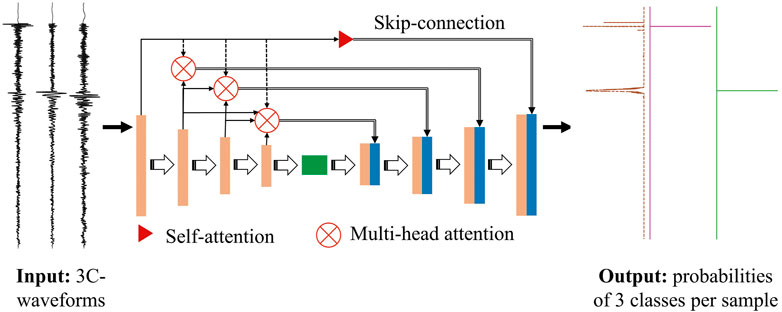
FIGURE 1. EPick model architecture. The model inputs are three-component seismic waveforms of 1-min duration with a sampling rate of 100 Hz, so the input size is 6,000*3. The colored blocks represent different layers of the neural network, where the extracted features will go through sets of transformations. The whole architecture can be broadly divided into an encoder and a decoder. The encoder consists of several down-sampling operations (including a 1D convolution block and max pooling). For the encoder blocks, we adopt 32, 32, 32, 64, 64, 128 feature maps with a stride of 1 and padding, where the rectified linear unit (ReLU) is used as an activation function. Then, each of the first four blocks is followed by the max pooling operation with a stride of 2, 4, 4, 4, and a dropout of 0.2. The decoder contains several up-sampling processes conducted by 1D-deconvolution layers to recover the feature length of the previous stage, in which each block has the same size as the block in the encoder. The skip connection after the attention mechanism at each stage enables the network to concatenate the low-level features to the right block, where the built-in attention block in TensorFlow (Abadi et al., 2016) is used. Here, the skip connection directly copies the output of the attention mechanism (denoted as blue modules) to the right layer. The last layer adopts the classical softmax function to scale the probabilities of noise, first P-pick, and first S-pick per sample within 0–1 that are labeled as different color lines from left to right, which also has a size similar to the input.
UNet was originally proposed to perform biomedical image segmentation (Ronneberger et al., 2015). It mainly consists of a contracting path and an expanding path, which shares a similar spirit with the encoder–decoder architecture. The encoder comprises several convolution modules to encode the input with feature representations of multiple different levels, where each convolution module is followed by a max pool down-sampling operation. The decoder is comprises several deconvolutional modules to perform upsampling associated with concatenation operations and aims to semantically project the higher-resolution features extracted by the encoder into upsampled feature space to perform a dense classification.
The attention mechanism was first developed and extensively applied in the area of natural language processing to enhance the performance of the encoder–decoder-driven machine translation system (Vaswani et al., 2017). It succeeds in splitting complex tasks into small regions of attention and then processing those small tasks sequentially. Recently, this mechanism (including its variants) has achieved superior performance in a wide range of applications, including computer vision and speech processing. The two most common attention techniques used are self-attention and multi-head attention.
• Self-attention relates different positions of a single sequence to compute a representation of the sequence (Vaswani et al., 2017). It enables the input to interact with itself, calculate the attention scores, and finally achieve the aggregated output by using these interactions and attention scores. The attention scores are calculated by the dot-product attention module where the input interacts with each other. As illustrated in Vaswani et al., (2017), given a query Q, a key K, and a value V, the scaled attention is formulated as follows, where dk is the key’s dimension.
• Unlike self-attention, where attention is only computed once, in the multi-head mechanism, the process of the scaled dot-product attention runs multiple times in parallel to improve the performance of the self-attention layer (Han et al., 2020). Those independent attention outputs are simply concatenated and linearly transformed into the expected dimensions (Vaswani et al., 2017), which can be mathematically formulated as the following equation.
where
In general, convolutional neural networks (CNNs) use an aggregated function over the receptive field according to the shared kernel values in the whole feature map. In contrast to CNNs, the self-attention block utilizes a weighted average operation using the learned attention weights. Hence, the flexibility enables the attention module to focus on different regions adaptively and capture more informative features. As reported in (Cordonnier et al., 2019), a multi-head self-attention layer with a sufficient number of heads can be at least as expressive as any convolutional layer.
Figure 1 shows the three-channel waveform represented by a three-channel 1-dimensional vector, which is fed as the input to EPick, which classifies each input data sample as one of the three classes: noise, first P-arrival, and first S-arrival. Here, each channel of the seismic waveform is sampled at 100 Hz for a 60-s time length. We label the output of our model as
When seismic data are fed into the neural network, it undergoes several downsampling and upsampling modules. Each module comprises a 1D convolutional block associated with a rectified linear unit (ReLU) activation function. These extracted features are forwarded to the upsampling stage such that at each moment, one can obtain the corresponding probability distribution over three classes.
A skip connection involving an attention block at each stage enables the concatenation of the features learned from the encoder part to the upsampling stage. Here, the attention blocks serve to allow the decoder to flexibly use the most relevant parts of the encoder’s hidden states by a weighted sum over those encoded input.
Similar to Zhu and Beroza, (2019), the deconvolution operation (Noh et al., 2015) is used to achieve upsampling to recover the previous feature size. Furthermore, padding operations are also performed before and after convolutions to keep the output size the same as the input size.
To output the probability distribution over three classes at each component for each sample, a softmax function (Goodfellow et al., 2016) is used as the final layer in the network. The fundamental process of the softmax module is to convert the output representation of the decoder part into probability between the intervals of (0, 1). Here, the detection process is regarded as a multiple classification problem. Hence, the results of EPick on each data sample are mapped into the probability by using a softmax function as
where i = 1, 2, 3 denotes the noise, first P-arrival, and first S-arrival, respectively; and zi(x) represents the unscaled output of EPick before using the softmax function for the ith class. Meanwhile, the cross-entropy (Murphy, 2012) between the ground truth probability p(x) and the predicted distribution q(x) is utilized to compute the loss
pi(j) and qi(j) denote the true and predicted probability distribution of the ith class and jth sample point, respectively, where i = {1, 2, 3} indicates the class label and j = {1, 2, … , n} denotes the sampling number.
Considering that the data used in this work have a class imbalance problem (Kaur et al., 2019), i. e., the class “noise” far exceeds the other two classes, which poses a challenge to building a reliable classification model statistically. In order to resolve this, a weight is introduced for each class, which helps the model place more emphasis on the minority classes during the model training process. It aims at ensuring a classifier that is capable of learning equally from all categories. Hence, the loss function is rewritten as
For this study, several subsets of the STanford EArthquake Dataset (STEAD) (Mousavi et al., 2019) are used to train and test the architecture of the EPick neural network. About 100,000 three-component waveforms, including both earthquake and noise waveforms, are used to train the proposed model. Here, the seismic event data are selected based on the unique source ID in the STEAD dataset. It should be noted that in contrast to previous studies such as (Zhu and Beroza, 2019; Liao et al., 2021), we do not use a time window format to mark the arrival times of P- and S-phases to train the model. The ratio between training and testing data is approximately 4 : 1. To evaluate the earthquake detection and phase picking performance of EPick, 25,000 seismic waveforms (including 20,000 earthquake and 5,000 pure-noise examples) are used as a test dataset, wherein a comparison is made between EPick and the baseline methods, including UNet without attention modules and AR picker (Akazawa, 2004). It should be noted that for comparison, the baseline model, UNet, is trained on the same training set and then applied to a common test set from STEAD. Figure 2A shows the earthquake magnitude distribution of the training and testing datasets, and Figure 2B gives an example of seismic data marked with phase arrival time. Figure 3 is used as an example of training instance visualizations of the earthquake and non-earthquake signals with their corresponding labels.
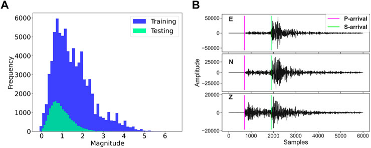
FIGURE 2. Data visualization in the analysis. (A) shows the frequency–magnitude distributions of earthquake events in the training dataset. (B) gives an example of a seismic data (Mousavi et al., 2019), where the plots in the figure from the top to the bottom represent the three-component seismic recordings (including east–west, north–south, and vertical directions), respectively. In (B), the colored vertical lines denote the first arrival times of picked P and S phases from the earthquake catalog, respectively.
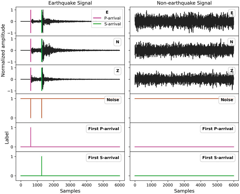
FIGURE 3. Visualization of training examples including one earthquake event and non-earthquake signal of the STEAD dataset (Mousavi et al., 2019). The three plots at the top of each subfigure in black color represent the normalized three-component seismograms, where the colored vertical lines denote the picked arrival time of P- and S-phase from the recorded earthquake catalog of the STEAD dataset (Mousavi et al., 2019). The bottom three plots denote the label information, where the label of each sample is encoded as a one-hot vector.
In the model testing phase, a time interval centered on the true phase picking time is employed to locate the predicted phase pick. The time interval for the first P arrival is ±0.1 s from the true label, while for the first S arrival, it is ±0.2 s. It should be noted that a larger time interval is chosen for first S arrival picking since the interference of P-wave signals with the later arriving shear waves makes it more difficult to pick first S arrival than first P arrival (Diehl et al., 2009). To test its robustness and generalization, EPick is also compared with previous methods on the INSTANCE dataset (Michelini et al., 2021). To evaluate the model performance, the confusion matrix (Sammut and Webb, 2011), a powerful analytical tool in deep learning and data science, is used, which is capable of displaying detailed information about how a deep learning classifier has performed with respect to the target classes in the dataset. Then, the following metrics, i.e., precision, recall, and F1-score, are defined.
where TP, TN, FP, and FN are the numbers of true-positive samples, true-negative samples, false-positive samples, and false-negative samples, respectively. In addition, picking error, referring to the time residuals t (also called “time difference”) between picks of the deep learning model and ground truth, is also used to evaluate arrival time picking error. In this work, EPick is constructed and implemented in TensorFlow (Abadi et al., 2016) and is trained and tested on an Nvidia A100 GPU. The Adam optimizer is used for optimizing the method. A dropout rate of 0.2 for the dropout layers is used in the training phase.
The overall detection performance for earthquake events is shown in Table 1. Both EPick and UNet are trained on the same dataset;whereas the recursive STA/LTA approach (Withers et al., 1998) requires no training process. Table 1 shows that EPick outperforms the traditional STA/LTA method and is slightly better in all categories than UNet (without using the attention mechanism).
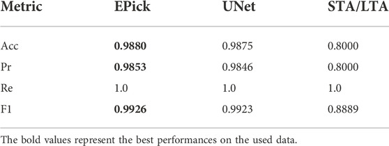
TABLE 1. Earthquake detection performance on the test data of the STEAD dataset (Mousavi et al., 2019). Acc is the overall classification accuracy. Pr, Re, and F1 are precision, recall, and F1-score respectively. Here, the recursive STA/LTA algorithm is utilized.
Table 2 lists the experimental results of EPick, UNet, and AR picker (Akazawa, 2004) tested in this study for seismic phase arrival time picking. The mean (μ) and standard deviation (σ) of arrival-time residuals between model-detected picks and ground truth picks are computed in seconds for model performance evaluation. The statistics described in Eq. 5 suggest that EPick achieves better performance over both UNet and AR picker when dealing with seismic phase picking.
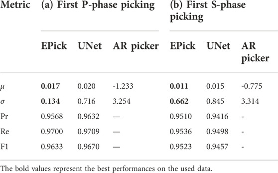
TABLE 2. First phase arrival-time picking on the test dataset from the STEAD dataset (Mousavi et al., 2019). μ and σ are the mean and standard deviation of the arrival time errors (prediction-ground truth) in seconds, respectively. Pr, Re, and F1 are precision, recall, and F1-score, respectively.
Figures 4A,B visualizes the earthquake event detection performance with the help of confusion matrices for UNet and EPick, respectively, where we can find that EPick has a low ratio for misclassification of noise events. Figures 4C,D display the distribution of picking errors between the predicted and ground truth first P and first S picks for EPick and UNet, respectively.
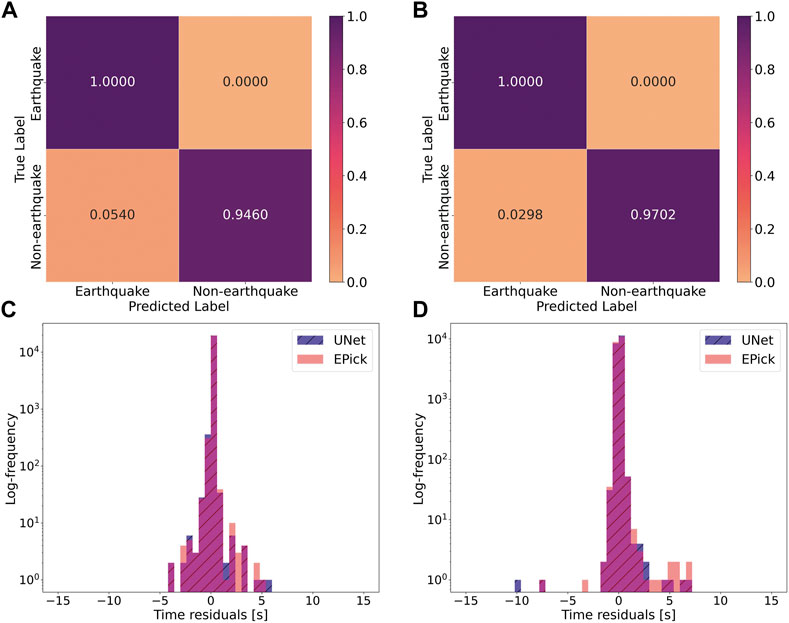
FIGURE 4. Result analysis for earthquake detection and phase arrival-time picking. (A,B) are confusion matrices for earthquake event detection in the testing data for UNet and EPick. During testing, EPick misclassifies less noise as earthquake events. (C,D) are the distributions of time residuals (also called time difference, Δt) for the first P and S picks of UNet and EPick on the test data set. Here, the histogram color under the overlap area of two distributions is different from that of the legend in (C,D).
In summary, from the abovementioned figures and tables, we can interpret that 1) the attention mechanism contributes to improving the performance of earthquake detection, and 2) for seismic phase picking, it helps the neural network focus more on the features related to phase picking, resulting in performance enhancement.
Moreover, PhaseNet (Zhu and Beroza, 2019) is retrained and tested on the same data from the STEAD dataset, where the parameter setting is kept the same as in the original article (Zhu and Beroza, 2019). In PhaseNet, a mask with the shape of a Gaussian distribution around the manual picks is used to label the P- and S- phases such that ground-truth arrival times could be centered on the manual picks with some uncertainty.
In contrast to PhaseNet (which picks the first arrivals of P-phase and S-phase), EPick is trained on noise signals as well, which makes it capable of detecting the earthquake and performing phase picking. It should be noted that the arrival-time residuals that are less than 0.1 s are regarded as true positives in PhaseNet. In this study, arrival-time residuals that are less than 0.1 s and 0.2 s are regarded as true positives for P-phase and S-phase, respectively. The same method used in PhaseNet is adopted to calculate precision, recall, and F1-score. Accordingly, the results are as follows: 1) for the first P-phase picking, the precision, recall, and F1-score and the mean and standard deviation of the arrival time errors of the PhaseNet are 0.981, 0.966, 0.973, -0.000 , and 0.088 s, respectively. The precision, recall, and F1-score and the mean and standard deviation of the arrival time errors of the EPick are 0.976, 0.970, 0.973, 0.011, and 0.019 s, respectively; 2) for the first S-phase picking, the precision, recall, and F1-score and the mean and standard deviation of the arrival time errors of the PhaseNet are 0.989, 0.968, 0.978, -0.009, and 0.114 s, respectively. The precision, recall, and F1-score and the mean and standard deviation of the arrival time errors of the EPick are 0.961, 0.954, 0.957, 0.000, and 0.053 s, respectively. The results show that 1) EPick has a lower standard deviation for the first P-phase picking than Phasenet for arrival-time error, whereas it achieves a comparable result in precision, recall, and F1-score, and 2) for the first S-phase picking, PhaseNet shows slightly better performance in precision, recall, and F1-score than EPick, while EPick has a lower mean and standard deviation for the arrival-time errors.
In deep learning, model generalization describes how well a trained model performs on unseen data. This is regarded as one of the most important criteria in practical applications. To investigate the generalization abilities on a separate dataset, the trained model is tested on a subset of the INSTANCE dataset (Michelini et al., 2021), where seismic waveform data are collected from weak and strong motion stations that have been extracted from the Italian EIDA node. Meanwhile, in the INSTANCE dataset, the arrival times of P-phase and S-phase are picked manually. Considering that the time interval of ±0.1 s is used in the PhaseNet model (Zhu and Beroza, 2019) for first P and S arrival picking, and in ARRU (Liao et al., 2021), the standard deviation of the target Gaussian function is 0.2 s for the P picks and 0.3 s for the S picks, which are used to label phase arrival time. In this study, we use the same time interval ±0.1 s for the P and S phases to denote the uncertainty interval in our model for evaluation of the model’s generalization on the INSTANCE dataset. It is worth noting that in the model training phase, single corresponding samples with the largest probability for each class are utilized as the ground truth arrival times for P and S waves in EPick, respectively, whereas the label in Gaussian format is used in both PhaseNet (Zhu and Beroza, 2019) and ARRU (Liao et al., 2021) during the model training phase.
Figure 5A shows the magnitude distribution of the used subset of INSTANCE data, and Figure 5B gives the example of one seismic event signal of different lengths, where dashed lines represent the length of the input fed into different models. It should be noted that, on one hand, seismic data with different time durations are used in ARRU, PhaseNet, and EPick, for example, 20-s data are used in ARRU (Liao et al., 2021), 30-s data are used in PhaseNet (Zhu and Beroza, 2019), and 60-s data are adopted in EPick. Hence, for this comparison, only the seismic data whose P and S arrival times are within the 20-s limit are considered. On the other hand, each raw seismic trace from the INSTANCE dataset has a length of 120 s. Therefore, the consecutive waveform within the duration time (e.g., 20 s, 30 s, and 60 s) after the trace starting time of each trace is selected for ARRU, PhaseNet, and EPick, respectively. Then, the clipped trace is further labeled by these three models. In addition, here, the used PhaseNet model (Zhu and Beroza, 2019) is directly cited from their saved trained models without re-training in this work.
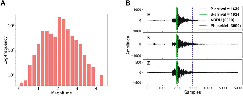
FIGURE 5. Magnitude distribution and seismic signal visualization of the used subset of the INSTANCE dataset (Michelini et al., 2021). (A) shows the frequency distribution of the test data magnitude, and (B) visualizes one 3-component seismic waveform marked with different time intervals. Here, a 60-s seismic waveform is sampled at 100 Hz. The evaluated models use different lengths of the same seismic event, marked with different dashed lines.
The model comparison results are shown in Table 3. The results demonstrate that EPick obtains better results in the first P-phase arrival picking on the INSTANCE dataset than AR picker (Akazawa, 2004) and PhaseNet (Zhu and Beroza, 2019), and it also achieves a comparable result with PhaseNet in the first S-phase picking. On the first S-phase arrival picking, the mean error and standard deviation of EPick are comparatively larger than the picking result of the first P-phase picking. The reason might be that a large weight is assigned to the first S-phase arrival pick during the model training. We also observed that by using similar weights for both the first P-phase and S-phase, the model performance on picking the first S-wave arrival worsens without any significant improvement in the P-phase picking error. Unlike PhaseNet, our proposed model is trained on non-earthquake signals, which leads to more robust performance.
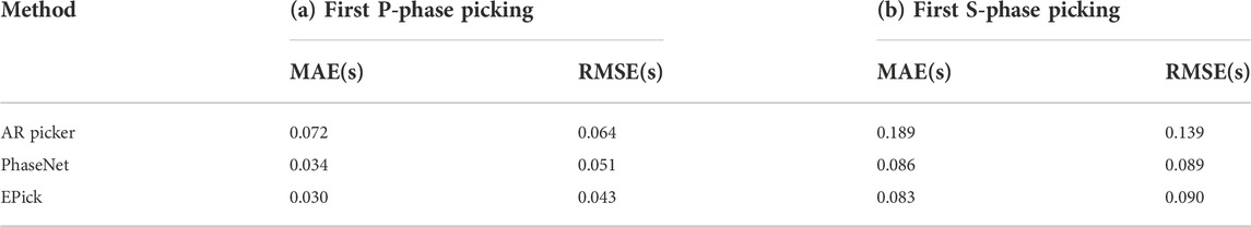
TABLE 3. Seismic phase picking on the INSTANCE dataset (Michelini et al., 2021). MAE and RMSE are the mean absolute error and root mean squared error of the arrival time errors (prediction-ground truth) in seconds, respectively. Here, the absolute arrival-time error below 0.5 s is considered.
In general, the visualization of representative results is useful for model analysis. To that end, one correctly classified example and three misclassified examples from the test dataset are plotted in Figure 6. Figure 6A shows an earthquake waveform that has been correctly classified as an earthquake; the peaks of the predicted probability distribution of EPick are very close to the manually picked first arrival times of P- and S-phases. The three misclassified examples are marked as ‘noise’ in the STEAD dataset (Mousavi et al., 2019) but are identified as earthquakes by the model. Figure 6B shows that EPick only picks a P-arrival and no S-arrival, this happens in case of 81.61% of noise waveforms misclassified as earthquakes, while in 7.69% of cases, only the S-arrival is picked. Thus, only for 10.70% of noise waveforms misclassified as earthquakes, both P- and S-arrivals are picked; two such examples are shown in Figures 6C,D. While the former actually resembles seismic noise, the latter appears to be very similar to a teleseismic event. It is worth noting that for each earthquake waveform, the model picks both P- and S-arrivals.
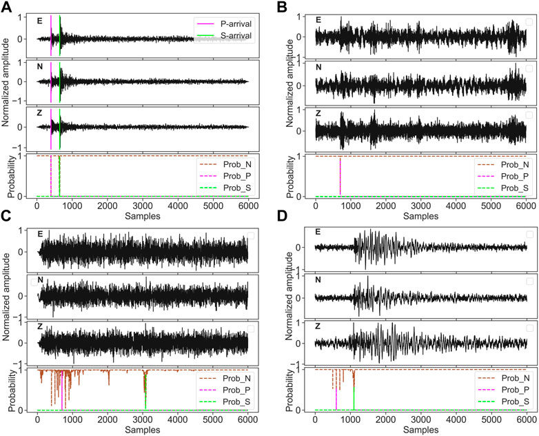
FIGURE 6. Visualization of a prediction example in the test dataset. (A) shows an earthquake waveform, correctly classified as an earthquake waveform. (B–D) show three misclassified examples, where the ground truth (according to the metadata) is non-earthquake, but the model classifies them as earthquake signals. In (B), only the P-phase is detected, while in (C,D), both P- and S-phases are detected. The first three sub-figures represent the three-component seismic recordings, namely, “E” (east–west), “N” (north–south) and “Z” (vertical direction), respectively. The bottom sub-figure plots the predicted probability corresponding to the three classes: “noise,” “P wave,” and “S wave.” The two colored vertical lines in the top sub-figures of (A) denote the first arrival times of P- and S-phases from the test dataset provided in the metadata.
The proposed model, EPick, is trained on the STEAD dataset that is band-pass filtered from 1.0 to 45.0 HZ (Mousavi et al., 2020). To investigate the impact of the denoising technique on model performance, a raw trace of low signal-to-noise ratio (SNR) from the INSTANCE dataset (Michelini et al., 2021) before and after filtering is fed into EPick for performance evaluation. Here, the band-pass filter from obspy. signal.filter (Beyreuther et al., 2010) is used with a frequency ranging from 1.0 to 40.0 Hz, and more details can be found in Figure 7 caption. Figure 7 shows the prediction result, for which it could be hard for experts to manually pick the first P-phase and S-phase arrival times. Figure 7 shows that EPick achieves good arrival time picking results with high probabilities. It further demonstrates that this kind of pre-processing procedure could not impact the performance of phase arrival time picking.
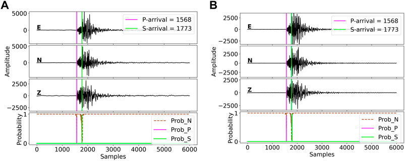
FIGURE 7. Output visualization of a low SNR data including (A) raw data and (B) data processed with a band-pass filter. For this trace example, the mean SNR over three components is 35.39 dB, with magnitude=1.5 and depth =9.8 km. The top three sub-figures represent the three-component seismic recordings, namely, ‘E’ (east–west), “N” (north–south), and “Z” (vertical direction), respectively. The bottom sub-figure plots the predicted probability corresponding to the three classes: “noise”, first P-wave, and first S-wave. The colored vertical lines in the top three sub-figures denote the first arrival times of P- and S-phases corresponding to the earthquake catalog of the used INSTANCE dataset.
In this study, we investigate the combination of raw UNet and attention mechanisms involving self-attention and multi-head attention for seismic phase picking. To fully leverage the power of the attention mechanism, a simple neural network architecture, EPick, is proposed, which not only completes the task of seismic event detection but also well-utilizes the low-level extracted features by using the UNet architectural design to achieve phase arrival time detection. As an alternative framework for seismic phase picking, EPick achieves superior performance compared to previously published methods for first S-phase arrival picking, whereas the performance is more robust in the case of the P-phase. The experimental results well-demonstrate the generalization ability of the proposed model in S-phase picking. In addition, the result with or without using the denoising technique shows that the model’s performance does not mainly rely on data filtering. This model can be used in tasks that require fast seismic data processing, as well as in dealing with big data. EPick can further be developed by monitoring real-time seismic signals.
In this work, the proposed model, EPick, mainly focuses on studying the important role of the attention mechanism in seismic phase picking by using a simple neural network architecture. In the future, EPick could be further extended to develop a more advanced model to circumvent the challenge of imbalanced data distribution with the use of a robust loss function, which aims at achieving better performance for both P-phase and S-phase arrival time picking.
The data used in this work including STEAD dataset and INSTANCE dataset are available at https://github.com/smousavi05/STEAD, and https://github.com/ingv/instance.
WL: conceptualization, methodology, coding, writing the first original draft, review, and editing. MC: suggestion in analysis, manuscript revision, and reading. DF: suggestion in analysis, manuscript revision, and reading. JF: suggestion in analysis, manuscript revision, and reading. KZ: suggestion in analysis, manuscript revision, and reading. GR: conceptualization, suggestion in analysis, and manuscript revision. HS: manuscript revision. NS: corresponding author, conceptualization, suggestion in analysis, writing sections in the manuscript, manuscript revision, and reading.
This research is supported by the “KI-Nachwuchswissenschaftlerinnen”—grant SAI 01IS20059 by the Bundesministerium für Bildung und Forschung—BMBF. Calculations were performed at the Frankfurt Institute for Advanced Studies’ new GPU cluster, funded by BMBF for the project Seismologie und Artifizielle Intelligenz (SAI).
We also thank Dr. Jan Steinheimer, Dr. Claudia Quinteros Cartaya, and Jonas Köhler for their kind suggestions. We would also like to thank the four reviewers for their insightful comments.
The authors declare that the research was conducted in the absence of any commercial or financial relationships that could be construed as a potential conflict of interest.
All claims expressed in this article are solely those of the authors and do not necessarily represent those of their affiliated organizations, or those of the publisher, the editors, and the reviewers. Any product that may be evaluated in this article, or claim that may be made by its manufacturer, is not guaranteed or endorsed by the publisher.
Abadi, M., Barham, P., Chen, J., Chen, Z., Davis, A., Dean, J., et al. (2016). “Tensorflow: A system for large-scale machine learning,” in 12th USENIX symposium on operating systems design and implementation (OSDI 16), 265–283.
Akazawa, T. (2004). “A technique for automatic detection of onset time of p-and s-phases in strong motion records,” in Proc. Of the 13th world conf. On earthquake engineering (Vancouver, Canada), 786.
Allen, R. V. (1978). Automatic earthquake recognition and timing from single traces. Bull. Seismol. Soc. Am. 68, 1521–1532. doi:10.1785/bssa0680051521
Álvarez, I., García, L., Mota, S., Cortés, G., Benítez, C., and De la Torre, Á. (2013). An automatic p-phase picking algorithm based on adaptive multiband processing. IEEE Geosci. Remote Sens. Lett. 10, 1488–1492. doi:10.1109/lgrs.2013.2260720
Bai, C.-y., and Kennett, B. (2000). Automatic phase-detection and identification by full use of a single three-component broadband seismogram. Bull. Seismol. Soc. Am. 90, 187–198. doi:10.1785/0119990070
Beyreuther, M., Barsch, R., Krischer, L., Megies, T., Behr, Y., and Wassermann, J. (2010). Obspy: A python toolbox for seismology. Seismol. Res. Lett. 81, 530–533. doi:10.1785/gssrl.81.3.530
Chakraborty, M., Fenner, D., Li, W., Faber, J., Zhou, K., Ruempker, G., et al. (2022). Creime: A convolutional recurrent model for earthquake identification and magnitude estimation. arXiv preprint arXiv:2204.02924.
Chakraborty, M., Rümpker, G., Stöcker, H., Li, W., Faber, J., Fenner, D., et al. (2021). “Real time magnitude classification of earthquake waveforms using deep learning,” in EGU general assembly conference abstracts. EGU21–15941.
Cordonnier, J.-B., Loukas, A., and Jaggi, M. (2019). On the relationship between self-attention and convolutional layers. arXiv preprint arXiv:1911.03584.
Cortes, C., Mohri, M., and Rostamizadeh, A. (2012). L2 regularization for learning kernels. arXiv preprint arXiv:1205.2653.
Diehl, T., Deichmann, N., Kissling, E., and Husen, S. (2009). Automatic s-wave picker for local earthquake tomography. Bull. Seismol. Soc. Am. 99, 1906–1920. doi:10.1785/0120080019
Fenner, D., Rümpker, G., Li, W., Chakraborty, M., Faber, J., Köhler, J., et al. (2022). Automated seismo-volcanic event detection applied to stromboli (Italy). Front. Earth Sci. (Lausanne). 267. doi:10.3389/feart.2022.809037
Goodfellow, I., Bengio, Y., and Courville, A. (2016). Deep learning. MIT Press. Available at: http://www.deeplearningbook.org.
Han, K., Wang, Y., Chen, H., Chen, X., Guo, J., Liu, Z., et al. (2020). A survey on visual transformer. arXiv preprint arXiv:2012.12556.
Hinton, G. E., Osindero, S., and Teh, Y.-W. (2006). A fast learning algorithm for deep belief nets. Neural Comput. 18, 1527–1554. doi:10.1162/neco.2006.18.7.1527
Kaur, H., Pannu, H. S., and Malhi, A. K. (2019). A systematic review on imbalanced data challenges in machine learning: Applications and solutions. ACM Comput. Surv. 52, 1–36. doi:10.1145/3343440
LeCun, Y., Bengio, Y., and Hinton, G. (2015). Deep learning. nature 521, 436–444. doi:10.1038/nature14539
Li, W., Rümpker, G., Stöcker, H., Chakraborty, M., Fenner, D., Faber, J., et al. (2021). “Mca-unet: Multi-class attention-aware u-net for seismic phase picking,” in EGU general assembly conference abstracts. EGU21–15841.
Li, W., Sha, Y., Zhou, K., Faber, J., Ruempker, G., Stoecker, H., et al. (2022). Deep learning-based small magnitude earthquake detection and seismic phase classification. arXiv preprint arXiv:2204.02870.
Liao, W.-Y., Lee, E.-J., Mu, D., Chen, P., and Rau, R.-J. (2021). Arru phase picker: Attention recurrent-residual u-net for picking seismic p-and s-phase arrivals. Seismol. Res. Lett. 92, 2410–2428. doi:10.1785/0220200382
Lomax, A., Satriano, C., and Vassallo, M. (2012). Automatic picker developments and optimization: Filterpicker—A robust, broadband picker for real-time seismic monitoring and earthquake early warning. Seismol. Res. Lett. 83, 531–540. doi:10.1785/gssrl.83.3.531
Michelini, A., Cianetti, S., Gaviano, S., Giunchi, C., Jozinovic, D., and Lauciani, V. (2021). Instance–the Italian seismic dataset for machine learning. Earth Syst. Sci. Data 13, 5509–5544. doi:10.5194/essd-13-5509-2021
Mousavi, S. M., Ellsworth, W. L., Zhu, W., Chuang, L. Y., and Beroza, G. C. (2020). Earthquake transformer–an attentive deep-learning model for simultaneous earthquake detection and phase picking. Nat. Commun. 11 (1), 3952. doi:10.1038/s41467-020-17591-w
Mousavi, S. M., Sheng, Y., Zhu, W., and Beroza, G. C. (2019). Stanford earthquake dataset (stead): A global data set of seismic signals for ai. IEEE Access 7, 179464–179476. doi:10.1109/access.2019.2947848
Nippress, S., Rietbrock, A., and Heath, A. (2010). Optimized automatic pickers: Application to the ancorp data set. Geophys. J. Int. 181, 911–925. doi:10.1111/j.1365-246x.2010.04531.x
Noh, H., Hong, S., and Han, B. (2015). “Learning deconvolution network for semantic segmentation,” in Proceedings of the IEEE international conference on computer vision, 1520–1528.
Pardo, E., Garfias, C., and Malpica, N. (2019). Seismic phase picking using convolutional networks. IEEE Trans. Geosci. Remote Sens. 57, 7086–7092. doi:10.1109/tgrs.2019.2911402
Ronneberger, O., Fischer, P., and Brox, T. (2015). “U-net: Convolutional networks for biomedical image segmentation,” in International Conference on Medical image computing and computer-assisted intervention (Springer), 234–241.
Sammut, C., and Webb, G. I. (2011). Encyclopedia of machine learning. Springer Science & Business Media.
Silver, D., Huang, A., Maddison, C. J., Guez, A., Sifre, L., Van Den Driessche, G., et al. (2016). Mastering the game of go with deep neural networks and tree search. nature 529, 484–489. doi:10.1038/nature16961
Sleeman, R., and Van Eck, T. (1999). Robust automatic p-phase picking: An on-line implementation in the analysis of broadband seismogram recordings. Phys. earth Planet. interiors 113, 265–275. doi:10.1016/s0031-9201(99)00007-2
Vaswani, A., Shazeer, N., Parmar, N., Uszkoreit, J., Jones, L., Gomez, A. N., et al. (2017). “Attention is all you need,” in Advances in neural information processing systems, 5998–6008.
Wang, J., Xiao, Z., Liu, C., Zhao, D., and Yao, Z. (2019). Deep learning for picking seismic arrival times. J. Geophys. Res. Solid Earth 124, 6612–6624. doi:10.1029/2019jb017536
Withers, M., Aster, R., Young, C., Beiriger, J., Harris, M., Moore, S., et al. (1998). A comparison of select trigger algorithms for automated global seismic phase and event detection. Bull. Seismol. Soc. Am. 88, 95–106. doi:10.1785/bssa0880010095
Xie, Z., Sato, I., and Sugiyama, M. (2020). Stable weight decay regularization. arXiv preprint arXiv:2011.11152.
Zhao, M., Chen, S., Fang, L., and David, A. Y. (2019). Earthquake phase arrival auto-picking based on u-shaped convolutional neural network. Chin. J. Geophys 62, 3034–3042. doi:10.6038/cjg2019M0495
Zhou, Y., Yue, H., Kong, Q., and Zhou, S. (2019). Hybrid event detection and phase-picking algorithm using convolutional and recurrent neural networks. Seismol. Res. Lett. 90, 1079–1087. doi:10.1785/0220180319
Zhu, L., Peng, Z., McClellan, J., Li, C., Yao, D., Li, Z., et al. (2019). Deep learning for seismic phase detection and picking in the aftershock zone of 2008 M7.9 Wenchuan Earthquake. Phys. Earth Planet. Interiors 293, 106261. doi:10.1016/j.pepi.2019.05.004
Keywords: earthquake detection, seismic phase picking, deep learning, u-shape neural network, attention mechanism
Citation: Li W, Chakraborty M, Fenner D, Faber J, Zhou K, Rümpker G, Stöcker H and Srivastava N (2022) EPick: Attention-based multi-scale UNet for earthquake detection and seismic phase picking. Front. Earth Sci. 10:953007. doi: 10.3389/feart.2022.953007
Received: 25 May 2022; Accepted: 25 October 2022;
Published: 17 November 2022.
Edited by:
Dun Wang, China University of Geosciences Wuhan, ChinaReviewed by:
Yu Ziye, Institute of Geophysics, China Earthquake Administration, ChinaCopyright © 2022 Li, Chakraborty, Fenner, Faber, Zhou, Rümpker, Stöcker and Srivastava. This is an open-access article distributed under the terms of the Creative Commons Attribution License (CC BY). The use, distribution or reproduction in other forums is permitted, provided the original author(s) and the copyright owner(s) are credited and that the original publication in this journal is cited, in accordance with accepted academic practice. No use, distribution or reproduction is permitted which does not comply with these terms.
*Correspondence: Nishtha Srivastava, c3JpdmFzdGF2YUBmaWFzLnVuaS1mcmFua2Z1cnQuZGU=
Disclaimer: All claims expressed in this article are solely those of the authors and do not necessarily represent those of their affiliated organizations, or those of the publisher, the editors and the reviewers. Any product that may be evaluated in this article or claim that may be made by its manufacturer is not guaranteed or endorsed by the publisher.
Research integrity at Frontiers
Learn more about the work of our research integrity team to safeguard the quality of each article we publish.