Tri-clustering–based exploration of spatio-temporal heterogeneity of six criteria air pollutants and their relationships in China

Severe air pollution in China has become a challenging issue because of its adverse health effects. The distribution of air pollutants and their relationships exhibits spatio-temporal heterogeneity due to influences by meteorological and socioeconomic factors. Investigation of spatio-temporal variations of criteria air pollutants and their relationships, thus, helps understand the current status and further assist pollution prevention and control. Even though many studies have been conducted, relationships among pollutants are non-linear due to complicated chemical reactions and were difficult to model by linear analyses in previous studies. Here, we presented a tri-clustering–based method, the Bregman cuboid average tri-clustering algorithm with I-divergence (BCAT_I), to explore spatio-temporal heterogeneity of air pollutants and their relationships in China. Concentrations of PM_2.5, PM₁₀, CO, SO₂, NO₂, and O₃ in 31 provincial cities in 2021 were used as the case study dataset. Results showed that air pollutants except O₃ exhibited spatial and seasonal variations, i.e., low in summer in southern cities and high in winter in northern cities. Variations of PMs were more similar to those of CO than other pollutants in southern cities in 2021. Results also found that relationships among these air pollutants were heterogeneous in different regions and time periods in China. Moreover, with the increasing level of NO₂ from summer to winter in northern cities, concentrations of O₃ first decreased and then increased. This is because the response of O₃ to NO₂ was negative at the low pollution level due to the titration reaction, which, however, changed to positive when concentrations of NO₂ became high.

Introduction

Severe air pollution in China, along with the rapidly growing economy, has become a concerning issue due to its adverse health impacts (Jin et al., 2018; Kim et al., 2018). Primary air pollutants include inhalable particles, such as PM_2.5 and PM₁₀ (fine particulate matters with diameters less than 2.5 and 10 $\mu \mathrm{m}$, respectively), and gaseous pollutants, including CO, SO₂, NO₂, and O₃. Particulate matters (PMs), i.e., PM_2.5 and PM_10, can penetrate deep into the lungs once inhaled and increase the susceptibility to respiratory and cardiovascular diseases (Gordon et al., 2018; Giani et al., 2020; Tainio et al., 2021). Exposure to gaseous pollutants also increases health risks by aggravating chronic respiratory diseases, exacerbating cardiovascular diseases, and weakening lung defense systems in the long term (Kampa and Castanas 2008; Mannucci and Franchini 2017). Thus, exploring variations of these air pollutants is essential to understand the current air pollution status in China and further assist pollution prevention and control for local and central government agencies. Since gaseous pollutants are the main precursors of PMs by enhancing the formation of secondary aerosols (Blanchard, 2003; Kota et al., 2018; Squizzato et al., 2018), the exploration and understanding of relationships among these air pollutants is also important to support decision-making.

Since the formation of both air pollutants and their precursors is influenced by meteorological and socioeconomic factors, distributions of air pollutants and their relationships are heterogeneous across both space and time (Cogliani, 2001; Fecht et al., 2015; He et al., 2017). Chai et al. (2014) explored spatio-temporal variations of these air pollutants in China in 26 cities from August 2011 to February 2012 and found that high pollution levels typically existed in northern cities, especially in winter, because of strong emissions from coal combustion in the heating period and poor weather conditions for dilution. They also observed high concentrations in city clusters, e.g., Beijing–Tianjin–Hebei in northern China, due to rapid urbanization. He et al. (2017) analyzed spatio-temporal heterogeneity of these pollutants in major Chinese cities during 2014–2015 and found that dispersion of pollution was determined by large-scale weather conditions and local meteorology. Xu et al. (2019) explored spatio-temporal variations of major air pollutants in China during 2005–2016 and identified significant spatial heterogeneity of air pollution caused by unbalanced regional economic development.

A few works also studied spatial and temporal heterogeneity of relationships among air pollutants in China. Wang et al. (2014) analyzed spatio-temporal variations of relationships among these six air pollutants in 31 provincial cities in China during 2013–2014 using the Pearson correlation coefficients. Seasonable variations were identified with high correlations among pollutions in winter due to strong formation of secondary PMs. Zhang et al. (2018) characterized spatial and temporal heterogeneity of relationships between air pollutants influenced by meteorological and geographical conditions by gray correlation analysis. Liu et al. (2021) explored spatio-temporal changes in relationships among pollutants by Pearson correlation analysis and identified seasonal variations because of weather conditions. In addition to being spatially and temporally heterogeneous, relationships among these air pollutants are also non-linear due to complex chemical reactions, which refer to the concurrent formation of different air pollutants (Wang et al., 2014; Chu et al., 2015; Abdullah et al., 2019). For instance, reactions of NO₂ and O₃ generate NO₃ and N₂O₅, which are the main contributors to form PMs (Healy et al., 2010; Zhang et al., 2018). Then, small reductions in NO_x emissions could lead to rising concentrations of O₃ due to the photochemical regime limited by the intermediate-volatility organic compounds (NMVOCs), i.e., the NMVOC-limited regime. A significant reduction in NO_x emissions, nonetheless, would change the regime from NMVOC-limited to NO_x-limited, which leads to the declination in concentrations of O₃ (Zhao et al., 2017; Womack et al., 2019). Such nonlinear relationships are difficult to explore using linear models in previous studies. Since air pollution is still a challenging issue in China, the exploration and reasonable understanding of the relationships is a prerequisite for effective control (Xing 2011).

Under this situation, tri-clustering methods can be used to explore non-linear relationships among air pollutants and also their spatio–temporal heterogeneity. Long et al. (2007) applied the tri-clustering method to analyze homogenous and heterogeneous relationships between different types of actors in IMDB movies. Gan et al. (2020) developed the tri-clustering method named TriPCE to investigate the varying relationships among different cancer types. Wu et al. (2018) developed a tri-clustering algorithm called the Bregman cuboid average tri-clustering algorithm with I-divergence (BCAT_I) to explore the complicated patterns in spatio-temporal data. Compared with one-way clustering (also known as traditional clustering) and co-clustering methods, tri-clustering methods simultaneously search clusters along three dimensions in 3D data and thereby enable the exploration of more complex patterns in the data (Wu et al., 2020). By formatting air pollutant datasets into a 3D data cube with locations, timestamps, and air pollutants as three dimensions, the tri-clustering methods partition the cube along three dimensions simultaneously (Figure 1). Then, by examining variations of air pollutants across space and time and also responses of air pollutants among each other along with these variations, non-linear relationships among air pollutants and their spatio-temporal heterogeneity can be explored.

FIGURE 1

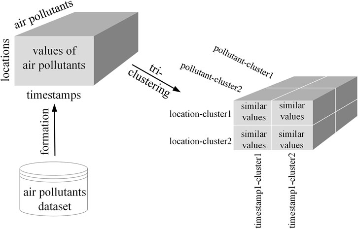
FIGURE 1. Tri-clustering analysis of air pollutants.

Data and methods

In this section, the case study dataset is first introduced. Then, the specific tri-clustering algorithm, BCAT_I, used for analyzing the dataset is described in detail.

Data

To illustrate the tri-clustering analysis in this study, data on PM_2.5, PM₁₀, CO, SO₂, NO₂, and O₃ collected from monitoring stations in 31 municipalities and provincial cities in the Chinese mainland (Figure 2) were used. Concentrations of these air pollutants were measured by the automatic monitoring systems installed at each station, according to the National Environmental Protection Standards HJ 193-2013 (MEP 2013) and HJ 655-2013 (MEP 2013). Monthly concentrations of these air pollutants in 2021 were obtained for free from the website of the China Air Quality Monitoring and Analysis Online Platform (https://www.aqistudy.cn/historydata/). For the tri-clustering analysis, normalization was performed on concentrations of each pollutant to [0 1] to assure the same scale.

FIGURE 2

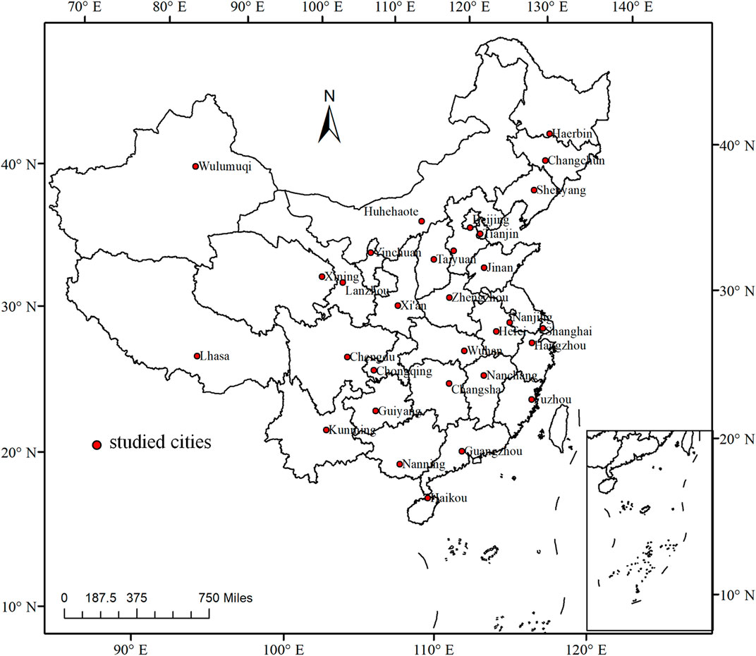
FIGURE 2. Geographic locations of 31 studied cities in China.

Bregman cuboid average tri-clustering algorithm with I-divergence

Bregman cuboid average tri-clustering algorithm with I-divergence (BCAT_I) allows the clustering analysis of any 3D data cube with positive and real values. The case study dataset was used to exemplify the optimization procedure of the tri-clustering algorithm. The formatted 3D data cube of the monthly concentrations of air pollutants can be seen as a 3D concurrence matrix O_SMP among three variables: the station variable S taking values in 31 stations, the month variable M taking values in 12 months, and the pollutant variable P taking values in six air pollutants. Accordingly, the tri-clustered data cube can be seen as another 3D concurrence matrix ${\widehat{O}}_{SMP}$ among variables of station cluster $\widehat{S}$, month cluster $\widehat{M}$, and pollutant cluster $\widehat{P}$, which take values in z station clusters, l month clusters, and h pollutant clusters, respectively. As a member of the information theory family, BCAT_I measured the quantity of shared information among variables using mutual information and constructed the objective function by calculating the loss of mutual information between OSMP and ${\widehat{O}}_{SMP}$ with information divergence. Then, the algorithm optimized the objective function to obtain the optimal tri-clustering results. We have summarized the four main steps of the optimization procedure of BCAT_I (Figure 3) as follows.

1) Step 1: The initialization was performed by randomly mapping 31 stations to z station clusters, 12 months to l month clusters, and six air pollutants to h pollutant clusters.

2) Step 2: The loss of mutual information was computed before and after tri-clustering as the objective function. First, the tri-clustered data matrix ${\widehat{O}}_{SMP}$ was generated using the initialized cluster assignments in Step 1. The amount of information shared among three variables, i.e., mutual information before and after cluster assignments, was calculated as $I\left(S;M;P\right)$ and $I\left(\widehat{S};\widehat{M};\widehat{P}\right)$, respectively, where $I\left(;\right)$ is the mutual information among variables. The optimal tri-clustering results minimize the loss of mutual information before and after tri-clustering $I\left(S;M;P\right)-I\left(\widehat{S};\widehat{M};\widehat{P}\right)$, which can be measured using information divergence between the original and tri-clustered data cubes:

${\mathit{f}}_{\mathit{o}\mathit{b}\mathit{j}}={\mathit{D}}_{\mathit{I}}\left({\mathit{O}}_{\mathit{S}\mathit{M}\mathit{P}}\Vert {\widehat{\mathit{O}}}_{\mathit{S}\mathit{M}\mathit{P}}\right).$

Here, $D_I\left(\cdot \Vert \cdot \right)$ indicates the information divergence between two elements.

3) Step 3: The assignments of station clusters, month clusters, and pollutant clusters were updated to optimize the objective function. Each of the 31 stations was assigned to the station cluster, which yielded the lowest value of the objective function, and the station-cluster assignment was updated. Similarly, month-cluster and pollutant-cluster assignments were updated.

4) Step 4: The objective function was re-computed using the updated cluster assignments. The tri-clustered data matrix was re-generated using updated station clusters, month clusters, and pollutant clusters. Then, the objective function was re-computed. If the convergence was achieved, i.e., variation of the objective function in two consecutive iterations was smaller than a predefined threshold, the algorithm would yield the optimal tri-clustering results; otherwise, steps 3 to 4 were repeated until convergence.

FIGURE 3

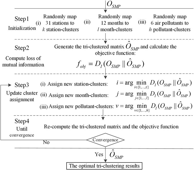
FIGURE 3. Optimization procedure of BCAT_I exemplified by monthly air pollutant data in 31 provincial cities of China.

It has been proved that the objective function decreases monotonically after each iteration (Banerjee et al., 2007), which assures the local convergence of BCAT_I. Nonetheless, random initialization was performed several times to maximize the likelihood of global convergence, and the one with the smallest loss of mutual information was finally selected. For a detailed explanation of BCAT_I, the study by Wu et al. (2018) can be referred to.

After the BCAT_I analysis, the air pollutant dataset was partitioned into z × l × h tri-clusters. Nevertheless, these tri-clusters might still have had similar values due to the predefinition of the cluster numbers (Wu et al., 2018). To solve this issue and refine the BCAT_I results, the k-means clustering algorithm was used to regroup these tri-clusters since it was proven to generate satisfactory results for the refinement of co-clustering/tri-clustering results (Wu et al., 2016; Wu et al., 2018). The mean and variance of each tri-cluster were used as input parameters for the algorithm to produce k axis-parallel but non-cubical tri-clusters.

Experiment design

As mentioned earlier, the air pollutants’ data cube with size 31 (stations) × 12 (months) × 6 (air pollutants) was first partitioned by BCAT_I into the z (station clusters) × l (month clusters) × h (pollutant clusters) data cube, which was then re-grouped by k-means into k final tri-clusters. The predetermination of numbers of clusters was needed by taking into account the case study dataset and also the purpose of the study (Table 1). In this study, the number of station clusters was set as three to divide the cities in the whole study area as severely, moderately, and slightly polluted cities, following the work of Zhao et al. (2016). The number of month clusters was set as four so that months could be partitioned into four “real” seasons to explore seasonal variations of air pollutants. The number of pollutant clusters was chosen as six, the same as the number of air pollutants, because the objective of this study was to explore the spatio-temporal heterogeneity of these air pollutants and their relationships, and thus, it was important to still distinguish these air pollutants after being processed by BCAT_I. The number of the final tri-clusters was set as six and optimized using the silhouette method that generated clustering results highly correlated with experts’ decisions (Lewis et al., 2012). These six tri-clusters were categorized as “lowest,” “medium-low,” “low,” “high,” “medium-high,” and “highest” in the order of increasing concentrations.

TABLE 1

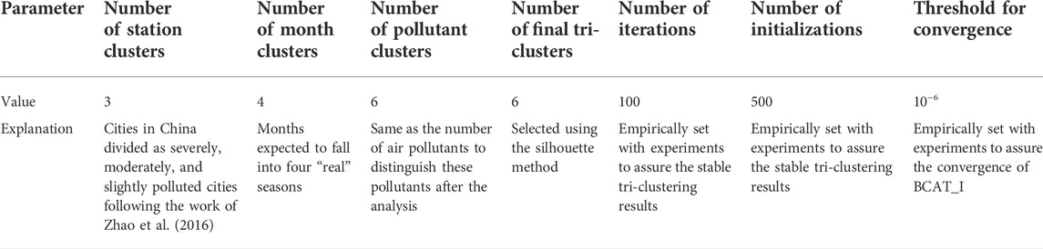
TABLE 1. Parameters for the tri-clustering analysis of the air pollutant dataset.

In addition, other parameters, i.e., the numbers of iterations and initializations and the threshold for convergence, were empirically selected using the case study dataset to assure the convergence of the tri-clustering analysis. Different settings of these parameters were used in experiments: the number of iterations from 50 to 100 with 10 as the interval, the number of initializations as 300, 400, and 500, and the threshold for convergence as 10⁻⁴ and 10⁻⁶ (Table 2). Experiments using the numbers of iterations from 50 to 80 yielded different tri-clustering results than the experiment using 100, which was because the convergence was not yet reached. As mentioned earlier, memberships of station clusters, month clusters, and pollutant clusters were first randomly assigned, which required a sufficient number of iterations for updating membership assignments to reach local convergence. The experiment using the number of iterations as 90 yielded similar results as the experiment using 100 but with a higher loss of mutual information. Experiments using different numbers of initialization yielded similar tri-clustering results, which means local convergence was reached, and the experiment using 500 was with the smallest loss of mutual information. Experiments using the threshold for convergence as 10⁻⁴ yielded similar results in combination with different initializations, while those using 10⁻⁶ mostly yielded the same results with a smaller loss of mutual information. This is because the criterion for convergence was loosened with a higher value of the threshold. Finally, the numbers of iterations and initializations and the threshold for convergence were selected as 100, 500, and 10⁻⁶ (Table 1).

TABLE 2

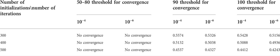
TABLE 2. Loss of mutual information with different settings of numbers of iterations and initializations and the threshold for convergence for the air pollutant dataset.

After the tri-clustering analysis, these six tri-clusters were visualized from different perspectives to display the spatio-temporal heterogeneity of the six air pollutants and their relationships (Figure 4). As to the perspective of pollutant clusters, a set of heatmaps was used to visualize variations of each air pollutant along station clusters and month clusters to uncover spatial and temporal heterogeneity of air pollutants (Figure 4A). As to the perspective of station clusters, a set of ringmaps was used to visualize variations of air pollutants along month clusters to uncover spatial heterogeneity of relationships among air pollutants (Figure 4B). As to the perspective of month clusters, another set of ringmaps was used to represent variations of air pollutants along station clusters to uncover temporal heterogeneity of relationships among air pollutants (Figure 4C).

FIGURE 4

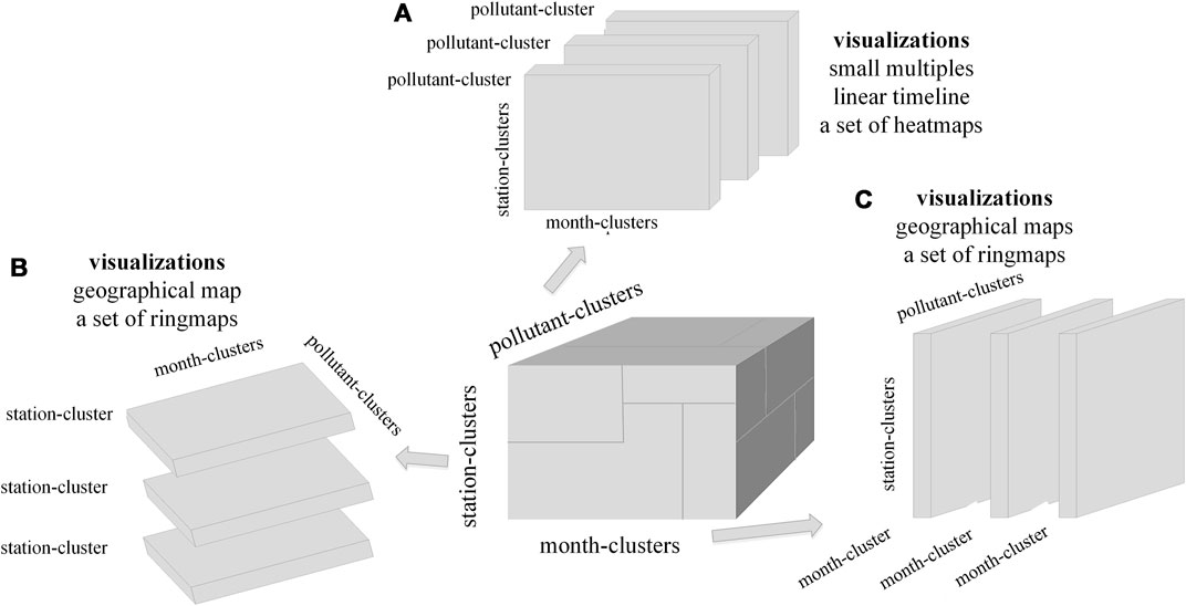
FIGURE 4. Exploration of tri-clustering results from different perspectives ((A): pollutants, (B): stations, (C): months) using the small multiples, linear timeline, heatmap, and ringmap.

Results

Overview of air pollutants

Based on the data on PM_2.5, PM₁₀, CO, SO₂, NO₂, and O₃ in 31 provincial cities in 2021, the distribution of these air pollutants is shown using the boxplot in Figure 5. In each boxplot, the bottom and top edges of the box represent the 25th (Q1) and 75th (Q3) quantiles of concentrations of corresponding air pollutants, and the upper and lower whiskers represent concentrations of $\mathrm{Q}1-1.5\times \left(\mathrm{Q}3-\mathrm{Q}1\right)$ and $\mathrm{Q}3+1.5\times \left(\mathrm{Q}3-\mathrm{Q}1\right)$ for corresponding pollutants. In addition, their spatial distribution in the study area and their temporal distribution over the 12 months in 2021 are displayed in Figure 6.

FIGURE 5

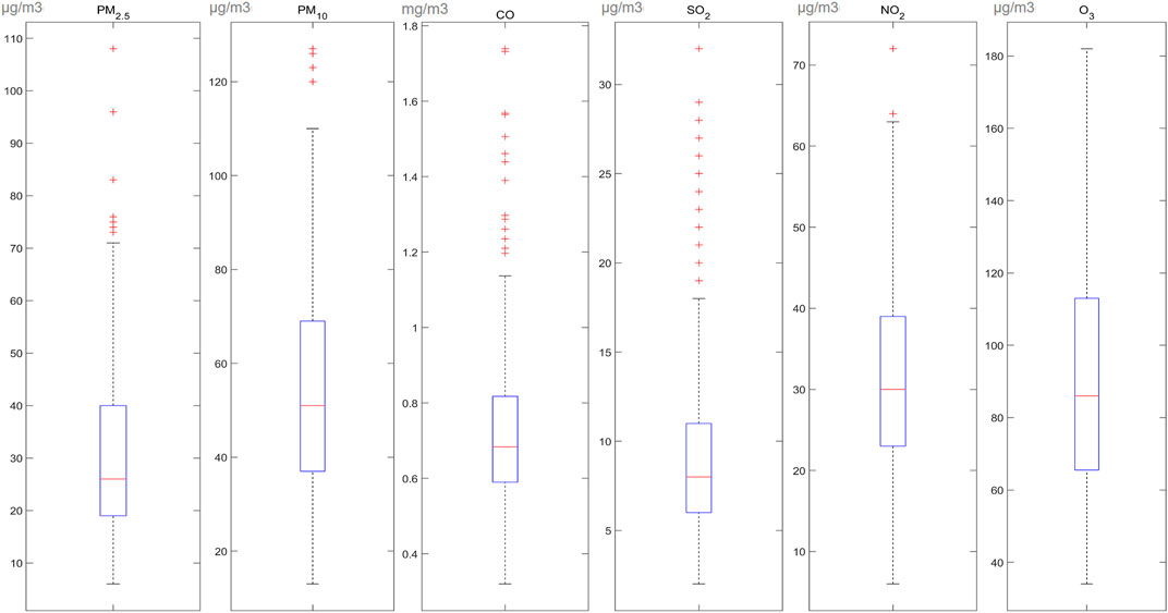
FIGURE 5. Distribution of concentrations for six criteria air pollutants.

FIGURE 6

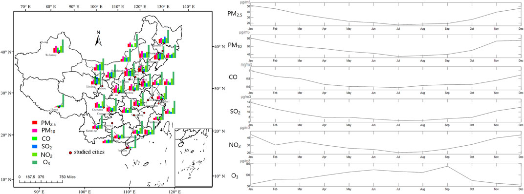
FIGURE 6. Spatial distribution of six air pollutants at 31 provincial cities in China and temporal distribution of pollutants for 12 months.

Concentrations of PM_2.5 ranged from 6 to $108\mu \mathrm{g}/\mathrm{m}3$, with an average of 31.18$\pm$16.61$\mu \mathrm{g}/\mathrm{m}3$. The annual average concentration in around 94% of these cities exceeded the Grade I standard (15 $\mu \mathrm{g}/\mathrm{m}3$) according to the Chinese ambient air quality (GB3095-2012, 2012), and around 40% of these cities exceeded the Grade II standard (35 $\mu \mathrm{g}/\mathrm{m}3$). Concentrations of PM₁₀ ranged from 13 to 127$\mu \mathrm{g}/\mathrm{m}3$, with an average of 55.27$\pm 22.74\mu \mathrm{g}/\mathrm{m}3$. The annual average concentration in more than 90% of these cities exceeded the Grade I standard (40 $\mu \mathrm{g}/\mathrm{m}3$) (GB3095-2012, 2012). High concentrations of PM_2.5 and PM₁₀ were mainly observed in northern and middle cities, e.g., Beijing, Jinan, and Tianjin, whereas low concentrations were distributed in southern cities, e.g., Haikou and Kunming. In the aspect of temporal distribution, PM_2.5 concentrations were high in the late autumn and winter, while they became low in spring and reached the bottom in summer. The temporal distribution of PM₁₀ was similar to that of PM_2.5 but with more variations.

Concentrations of CO ranged from 0.32 to 1.74$\mathrm{m}\mathrm{g}/\mathrm{m}3$ with an average of 0.72$\pm 0.21\mathrm{m}\mathrm{g}/\mathrm{m}3$, while the range of SO₂ concentrations was from 2 to 32$\mu \mathrm{g}/\mathrm{m}3$ with an average of 9.03$\pm 4.99\mu \mathrm{g}/\mathrm{m}3$. Concentrations of NO₂ ranged from 6 to 72$\mu \mathrm{g}/\mathrm{m}3$, with an average of 31$\pm 11.85\mu \mathrm{g}/\mathrm{m}3$. Similar to that of PMs, concentrations of CO, SO₂, and NO₂ increased from late autumn, peaked in winter, then decreased in spring, and reached the bottom in summer. Concentrations of O₃ ranged from 34 to 182$\mu \mathrm{g}/\mathrm{m}3$, with an average of 90.07$\pm 30.40\mu \mathrm{g}/\mathrm{m}3$. The temporal distribution of O₃ exhibited the opposite patterns compared with other air pollutants, whose concentrations were the lowest in winter, increased in spring, and peaked in summer.

Spatio-temporal heterogeneity of air pollutants

After the tri-clustering analysis, 31 stations, 12 months, and six air pollutants were grouped into three station clusters, four month clusters, and six pollutant clusters, respectively. The spatial distribution of station clusters, temporal distribution of month clusters, and variations of air pollutants are displayed in Figure 7.

FIGURE 7

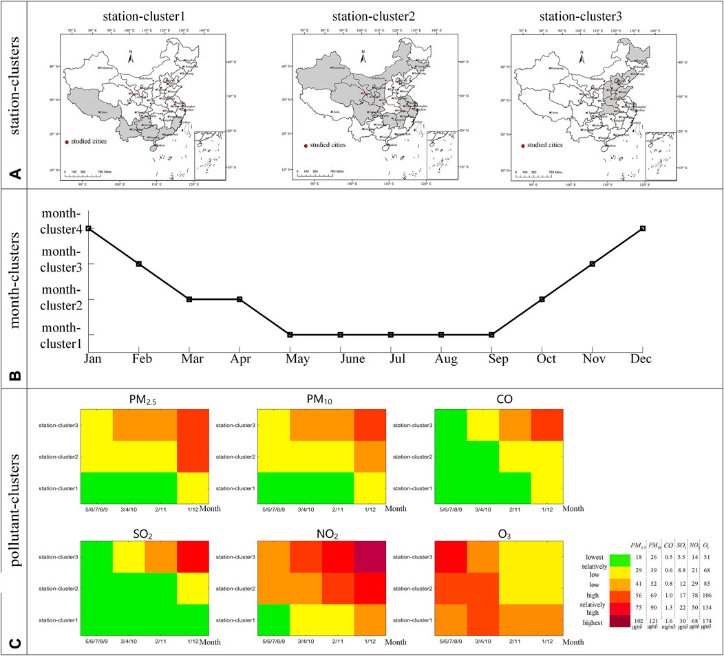
FIGURE 7. (A) Spatial distribution of station clusters with coverage indicated by provinces of corresponding cities (stations) in that station cluster, (B) temporal distribution of month clusters, and (C) variations of air pollutants.

Figure 7A displays the three station clusters as slightly, moderately, and severely polluted from station cluster 1 to station cluster 3. The spatial coverage of station clusters is indicated by provinces of corresponding cities (stations) in that station cluster by the gray color. Slightly polluted cities were mainly located in southern China, such as Haikou and Guangzhou. Moderately polluted cities were mainly distributed in middle and western China, such as Lanzhou and Chengdu, whereas severely polluted cities were distributed in the northern region, including Beijing and Shijiazhuang. Zhao et al. (2016) clustered the same 31 provincial cities according to the annual variation of these six air pollutants and obtained similar spatial distributions. Figure 7B shows the temporal distribution of the four month clusters, with an increasing level of pollution from month cluster 1 to month cluster 4. Elements in the month cluster 1 included May, months of summer, and September, which were the least polluted months. January and December were the most polluted months in 2021, which was supported by the temporal distribution of air pollutants in Figure 6, where concentrations of most air pollutants peaked in these 2 months.

Heatmaps in Figure 7C show variations of air pollutants across space and time after the tri-clustering analysis. These six categories of pollutants’ concentrations are represented by different colors and interpreted from the de-normalized values of the tri-clustered values for each corresponding air pollutant. Thus, it needs to be noticed that the same color indicates different values for different air pollutants. For instance, green as the “lowest” category indicates 18$\mu \mathrm{g}/\mathrm{m}3$ for PM_2.5, 26$\mu \mathrm{g}/\mathrm{m}3$ for PM₁₀, 0.5$\mathrm{m}\mathrm{g}/\mathrm{m}3$ for CO, 5.5$\mu \mathrm{g}/\mathrm{m}3$ for SO₂, 14$\mu \mathrm{g}/\mathrm{m}3$ for NO₂, and 51$\mu \mathrm{g}/\mathrm{m}3$ for O₃. Concentrations of PM_2.5 were the lowest in southern cities for all months in 2021 except January and December, which became high in spring and winter for northern cities and peaked in all cities in China except southern cities in January and December. Concentrations of PM₁₀ had similar variations with PM_2.5. Concentrations of CO were low in China in summer, increased in middle and western cities in winter, and peaked in the northern cities in winter. Concentrations of SO₂ had similar variations with CO, except that there were more low concentrations in all cities except northern cities in winter. Concentrations of NO₂ were high for almost all cities throughout the year. As expected, concentrations were the lowest in southern cities in summer and increased in northern cities in winter and finally peaked in January and December. The variation of O₃ was the opposite of that of other pollutants, with the lowest concentrations in all cities except southern cities in winter. Variations of CO and SO₂ were similar in all cities, especially in northern cities. In addition, variations of PM_2.5 and PM₁₀ were more similar to those of CO than other pollutants in cities in the southern region of China.

Spatial variations in concentrations of air pollutants except for O₃, i.e., low in southern cities and high in northern cities, and seasonal variations, i.e., low in summer and high in winter, are mainly due to emissions and meteorological conditions. Cities in the northern region of China generally have higher concentrations because of emissions from residential coal combustion and biomass burning for heating in winter (Wang et al., 2014; Li et al., 2017). More coal-based industries, such as coal-fired power plants, iron and steel manufacturing, and biomass burning–based domestic home heating in winter (from middle November through middle March), result in higher emissions and concentrations in the northern region (Zhao et al., 2011). In addition, weather conditions in winter, e.g., lower temperature, weaker winds, and less precipitation, further exacerbate air pollution due to poor diluted conditions, and less scavenging impacts of particles by precipitation lead to accumulation of pollutants and high concentrations of air pollutants (Zhao et al., 2016). As such, the slow winds and surface mixing layers in winter lead to high concentrations near the surface (Fu et al., 2018).

In contrast, high temperature, strong turbulent eddies, and more precipitation in summer could mitigate air pollution because of scavenging effects and favorable conditions of diffusing air pollutants by frequent rainfalls and appropriate conditions favoring pollutant diffusion (Li et al., 2019). Since the photochemical reaction to form O₃ is promoted by solar radiation, the seasonal variation of O₃, i.e., low in winter and high in summer, is because winter is with the minimum intensity of solar radiation (Pochanart 2015). By influencing the photolysis rate of NO₂ and the reaction rate coefficient of NO and O₃, high radiation duration and intensity in summer enhanced chemical reactions for O₃ (Zhang et al., 2018).

Spatio-temporal heterogeneity of relationships among air pollutants

Each ringmap in the first set of heatmaps in Figure 8 displays variations of PM_2.5, PM₁₀, CO, SO₂, NO₂, and O₃ from inside out for 12 months for each station cluster. The color scheme is the same as that used for heatmaps in Figure 7. Variations among these air pollutants are heterogeneous across space (station clusters). For slightly polluted cities in southern China (station cluster 1), variations of PM_2.5, PM₁₀, and CO were the same, with medium-low concentrations in January and the lowest concentrations in other months. The variation of SO₂ was also similar to that of the aforementioned three air pollutants but opposite to that of O₃. For cities in moderately polluted middle and western China (station cluster 2), PM_2.5 and PM₁₀ had similar variations, except that the pollution level of PM_2.5 was higher than that of PM₁₀. For cities in northern China (station cluster 3), variations of PM_2.5 and PM₁₀ were the same, with medium-low concentrations from May to September and high concentrations in January. Variations of CO and SO₂ were the same, with the lowest concentrations of air pollutants in summer, increasing in spring and autumn, and achieving the peak in January. Variations of PM_2.5 and PM₁₀ were similar to those of CO and SO₂ from October to December and from January to April, except that pollution levels of PM_2.5 and PM₁₀ in April and October were higher than those of CO and SO₂, which might be caused by dust events. Thus, relationships among air pollutants were varying at different regions.

FIGURE 8

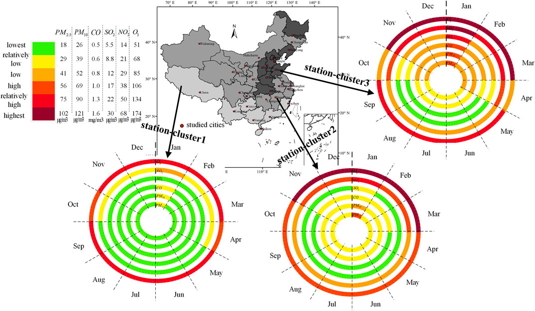
FIGURE 8. Spatial heterogeneity of relationships among six air pollutants from the perspective of station clusters; the map indicates spatial distribution of station clusters with coverage indicated by provinces of corresponding cities (stations) in that station cluster.

Each ringmap in the other set of heatmaps in Figure 9 displays the variation of these air pollutants from the inside out along all three station clusters for each month cluster. The color scheme is the same as that used for heatmaps in Figure 7 and Figure 8. Variations among other air pollutants were heterogeneous across time (month clusters). For most months in summer (month cluster 1), variations of PM_2.5 and PM₁₀ were the same, with the lowest concentrations in southern cities and increasing values in other cities. SO₂ and CO shared the same variations with the lowest concentrations for all cities. For spring and October, PM_2.5 and PM₁₀ had the same variations, with the lowest concentrations in southern cities, increasing in middle and western cities, and reaching the peak in northern cities. For February and November, variations of PM_2.5, PM₁₀, and CO were the same, with the lowest concentrations in southern cities and high concentrations in other cities, which are similar to those of SO₂. The variation of NO₂ was opposite to that of O₃. For January and December, the variation of PM_2.5 was similar to that of PM₁₀, which was also similar to those of CO, SO₂, and NO₂, with relatively low concentrations in southern cities and high concentrations in other cities. Variations of these air pollutants, except O₃, were closest to each other in January, which was typically the coldest month of the year. This is because these gaseous precursors were mainly generated from anthropogenic activities, e.g., coal and biomass burning for heating in this period, which directly contaminated the environment and also facilitated the formation of PM_2.5 (Liu et al., 2021).

FIGURE 9

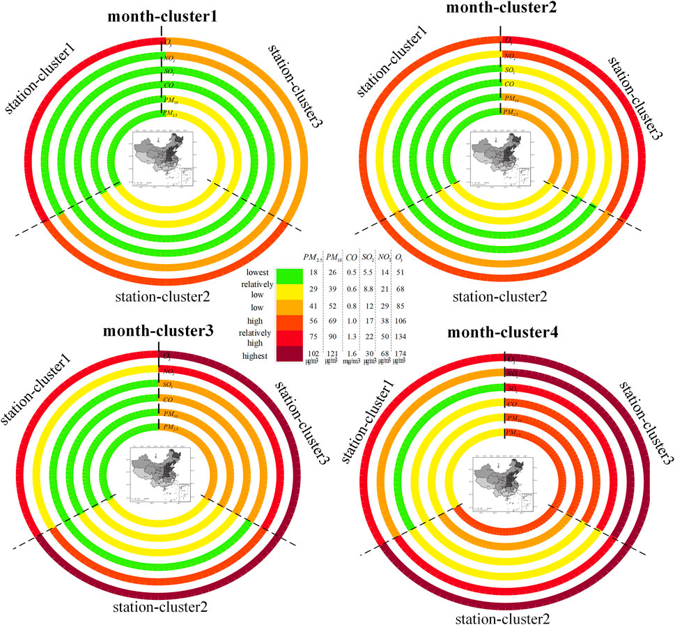
FIGURE 9. Temporal heterogeneity of relationships among six air pollutants from the perspective of month clusters; the map indicates spatial distribution of station clusters with coverage indicated by provinces of corresponding cities (stations) in that station cluster.

In addition, non-linear relationships among air pollutants can also be observed in the tri-clustering results. For instance, in the relationship between NO₂ and O₃, in southern cities where the pollution level was low, the variation of O₃ was similar to that of NO₂. However, in northern cities where the pollution level was high, with the increasing concentrations of NO₂ from summer to winter, concentrations of O₃ first decreased from September to October and then increased from autumn to winter. This is because the oxidation reaction of NO₂ resulted in O₃ depletion, and concentrations of NO₂ showed a negative contribution to O₃ at the low pollution level. Nonetheless, the response of O₃ changed from negative to positive when NO₂ reached a higher pollution level due to the existence of NMVOC (Xing et al., 2011).

Discussion

A few studies have applied the clustering analysis for exploring variations of air pollutants in China. For instance, Zhao et al. (2016) performed the clustering analysis of 31 provincial cities based on the annual and diurnal changes of six air pollutants from 2014 to 2015 and divided all cities into severely, moderately, and slightly polluted cities. Their results were supported by the spatial distribution of divided cities in this study (Figure 7A) that severely polluted cities were mainly located in the northern region, moderately polluted cities in middle and western regions, and slightly polluted cities in the southern region. Nonetheless, a bit of difference existed in the clustering results, i.e., Changchun belonged to the severely polluted city cluster in their study, whereas it was divided into the moderately polluted city cluster in this study, which might be caused by different study periods. Ye et al. (2018) applied a spatial clustering method to explore the hot spot areas of PM_2.5 in 338 Chinese cities and identified Beijing–Tianjin–Hebei and southwest Xinjiang as severely polluted areas. Although Beijing, Tianjin, and Shijiazhuang, the provincial city of Hebei, belonged to severely polluted cities in this study, Wulumuqi, the provincial city of Xinjiang, was divided as a moderately polluted city. The difference might be caused by the difference in the study area, i.e., 338 cities in their study and 31 cities in this study. In addition, many previous works have studied the spatial and temporal heterogeneity of air pollutants in China (Wang et al., 2014; He et al., 2017; Wang et al., 2017; Liang et al., 2019). These studies concluded that concentrations of air pollutants except O₃ are low in southern cities and high in northern cities, and low in summer and high in winter. Also, variations of PM_2.5, PM₁₀, CO, and SO₂ are similar in the whole study area and study period. These findings agree well with the results in our study that concentrations of air pollutants except O₃ were generally the lowest in summer, increased in northern and western cities in spring and autumn, and finally peaked in January and December (Figure 7). However, compared to findings reported by Wang et al. (2017) and Liang et al. (2019) that variations of PM_2.5 and PM₁₀ were more similar to those of CO than other pollutants in winter, results in this study found that variations of PM_2.5, PM₁₀, and CO were more similar than those of other pollutants in southern cities for the whole year (Figure 7C). This could be caused by the implementation of the “National Action Plan on Air Pollution Control” (State Council of the People’s Republic of China, 2013) from 2013 and the “Three-Year Action Plan for Winning the Blue Sky War” (State Council of the People’s Republic of China, 2018) from 2018 to 2020, as well as the consequent heterogeneous reactions in the atmosphere. In addition, in comparison with previous studies, the tri-clustering analysis in this study not only explored the spatio–temporal heterogeneity of air pollutants but also enabled the exploration of varying relationships among these air pollutants at the same time.

A few studies have analyzed the spatial and temporal heterogeneity of relationships among these air pollutants in China. Xie et al. (2015), Li et al. (2017), Zhang et al. (2018), and Liu et al. (2021) conducted the regional or national analysis of relationships among PM_2.5, PM₁₀, CO, SO₂, NO₂, and O₃ in China. These studies concluded that relationships among these air pollutants were heterogeneous in different cities and time periods. Such a conclusion was confirmed by the results of our study. Nonetheless, Zhao et al. (2016) found that variations of PMs were more similar to those of SO₂ than CO, which is different from the results in this study that CO shared similar variations with PMs other than SO₂. We suppose this is because of the different lengths of study periods and numbers of stations in the study area. Finally, compared with the aforementioned studies mainly using Pearson correlation analysis to explore relationships among pollutants, the tri-clustering analysis used in this study enabled the extraction of the non-linear relationships, e.g., with the increasing level of NO₂ in northern cities, concentrations of O₃ first decreased due to the titration reaction and then increased when the level of NO₂ was high. Since rapidly increasing ozone pollution has been noticed in recent years (Li et al., 2021), these findings could be helpful to support pollution control for local government agencies in northern cities.

Conclusion

In this study, we used the tri-clustering–based method to explore the spatial and temporal heterogeneity of air pollutants and their non-linear relationships in China. Concentrations of six criteria air pollutants, i.e., PM_2.5, PM₁₀, CO, SO₂, NO₂, and O₃, at 31 provincial cities in 2021 were used as the case study dataset. Our results showed that concentrations of air pollutants except O₃ exhibited spatial variations, i.e., low in southern cities and high in northern cities, and seasonal variations, i.e., low in summer and high in winter. Variations of PMs and CO were more similar than those of other pollutants in southern cities in 2021. Results also concluded that relationships among these air pollutants were heterogeneous in different regions and time periods in China. Moreover, our results found that with the increasing level of NO₂ in northern cities, concentrations of O₃ first decreased due to the titration reaction and then increased when concentrations of NO₂ became high. The future work mainly includes two directions: 1) in this study, only data on air pollutants from 31 municipalities and provincial cities in China were used; thus, in future work, it is recommended that data from individual sites across provinces could also be collected to enrich the case study dataset before being processed by the tri-clustering method; 2) since spatio–temporal heterogeneity also exists in relationships among air pollutants and their driving forces, e.g., meteorological and socio-economic factors (Zhao et al., 2018; Jin et al., 2019), in future work, it is thus recommended to apply the tri-clustering based analysis to the visual exploration of the spatio–temporal heterogeneity of air pollutants and their driving factors.

Data availability statement

The original contributions presented in the study are included in the article/Supplementary Material; further inquiries can be directed to the corresponding author.

Author contributions

XW is in charge of conceptualization, data analysis, writing, and editing.

Funding

This research was funded by the National Natural Science Foundation of China, grant numbers 42030509 and 41901317.

Conflict of interest

The author declares that the research was conducted in the absence of any commercial or financial relationships that could be construed as a potential conflict of interest.

Publisher’s note

All claims expressed in this article are solely those of the authors and do not necessarily represent those of their affiliated organizations, or those of the publisher, the editors, and the reviewers. Any product that may be evaluated in this article, or claim that may be made by its manufacturer, is not guaranteed or endorsed by the publisher.

References

Abdullah, S., Ismail, M., Ahmed, A. N., and Abdullah, A. M. (2019). Forecasting particulate matter concentration using linear and non-linear approaches for air quality decision support. Atmosphere 10 (11), 667. doi:10.3390/atmos10110667

CrossRef Full Text | Google Scholar

Banerjee, A., Dhillon, I., Ghosh, J., Merugu, S., and Modha, D. S. (2007). A generalized maximum entropy approach to bregman co-clustering and matrix approximation. J. Mach. Learn. Res. 8, 1919–1986.

Google Scholar

Blanchard, C. L. (2003). Spatial and temporal characterization of particulate matter. California, USA: California Environmental Protection Agency, Air Resources Board.

Google Scholar

Chai, F., Gao, J., Chen, Z., Wang, S., Zhang, Y., Zhang, J., et al. (2014). Spatial and temporal variation of particulate matter and gaseous pollutants in 26 cities in China. J. Environ. Sci. 26 (1), 75–82. doi:10.1016/s1001-0742(13)60383-6

PubMed Abstract | CrossRef Full Text | Google Scholar

Chu, H.-J., Huang, B., and Lin, C.-Y. (2015). Modeling the spatio-temporal heterogeneity in the PM10-PM2. 5 relationship. Atmos. Environ. 102, 176–182. doi:10.1016/j.atmosenv.2014.11.062

CrossRef Full Text | Google Scholar

Cogliani, E. (2001). Air pollution forecast in cities by an air pollution index highly correlated with meteorological variables. Atmos. Environ. 35 (16), 2871–2877. doi:10.1016/s1352-2310(01)00071-1

CrossRef Full Text | Google Scholar

Fecht, D., Fischer, P., Fortunato, L., Hoek, G., De Hoogh, K., Marra, M., et al. (2015). Associations between air pollution and socioeconomic characteristics, ethnicity and age profile of neighbourhoods in England and The Netherlands. Environ. Pollut. 198, 201–210.

PubMed Abstract | CrossRef Full Text | Google Scholar

Fu, W., Chen, Z., Zhu, Z., Liu, Q., den Bosch, V., Konijnendijk, C. C., et al. (2018). Spatial and temporal variations of six criteria air pollutants in Fujian Province, China. Int. J. Environ. Res. Public Health 15 (12), 2846. doi:10.3390/ijerph15122846

CrossRef Full Text | Google Scholar

Gan, Y., Li, N., Xin, Y., and Zou, G. (2020). TriPCE: A novel tri-clustering algorithm for identifying pan-cancer epigenetic patterns. Front. Genet. 10, 1298. doi:10.3389/fgene.2019.01298

PubMed Abstract | CrossRef Full Text | Google Scholar

GB3095-2012 (2012). Chinese ambient air quality (GB3095-2012). China: MEP.

Google Scholar

Giani, P., Castruccio, S., Anav, A., Howard, D., Hu, W., and Crippa, P. (2020). Short-term and long-term health impacts of air pollution reductions from COVID-19 lockdowns in China and europe: A modelling study. Lancet Planet. Health 4 (10), e474–e482. doi:10.1016/s2542-5196(20)30224-2

PubMed Abstract | CrossRef Full Text | Google Scholar

Gordon, T., Balakrishnan, K., Dey, S., Rajagopalan, S., Thornburg, J., Thurston, G., et al. (2018). Air pollution health research priorities for India: Perspectives of the indo-US communities of researchers. Environ. Int. 119, 100–108. doi:10.1016/j.envint.2018.06.013

PubMed Abstract | CrossRef Full Text | Google Scholar

He, J., Gong, S., Yu, Y., Yu, L., Wu, L., Mao, H., et al. (2017). Air pollution characteristics and their relation to meteorological conditions during 2014–2015 in major Chinese cities. Environ. Pollut. 223, 484–496. doi:10.1016/j.envpol.2017.01.050

PubMed Abstract | CrossRef Full Text | Google Scholar

Healy, R. M., Hellebust, S., Kourtchev, I., Allanic, A., O'Connor, I. P., Bell, J. M., et al. (2010). Source apportionment of PM<sub>2.5</sub> in Cork Harbour, Ireland using a combination of single particle mass spectrometry and quantitative semi-continuous measurements. Atmos. Chem. Phys. 10 (19), 9593–9613. doi:10.5194/acp-10-9593-2010

CrossRef Full Text | Google Scholar

Jin, G., Fu, R., Li, Z., Wu, F., and Zhang, F. (2018). CO2 emissions and poverty alleviation in China: An empirical study based on municipal panel data. J. Clean. Prod. 202, 883–891. doi:10.1016/j.jclepro.2018.08.221

CrossRef Full Text | Google Scholar

Jin, J.-Q., Du, Y., Xu, L.-J., Chen, Z.-Y., Chen, J.-J., Wu, Y., et al. (2019). Using Bayesian spatio-temporal model to determine the socio-economic and meteorological factors influencing ambient PM2. 5 levels in 109 Chinese cities. Environ. Pollut. 254, 113023. doi:10.1016/j.envpol.2019.113023

PubMed Abstract | CrossRef Full Text | Google Scholar

Kampa, M., and Castanas, E. (2008). Human health effects of air pollution. Environ. Pollut. 151 (2), 362–367. doi:10.1016/j.envpol.2007.06.012

PubMed Abstract | CrossRef Full Text | Google Scholar

Kim, D., Chen, Z., Zhou, L. F., and Huang, S. X. (2018). Air pollutants and early origins of respiratory diseases. Chronic Dis. Transl. Med. 4 (2), 75–94. doi:10.1016/j.cdtm.2018.03.003

PubMed Abstract | CrossRef Full Text | Google Scholar

Kota, S. H., Guo, H., Myllyvirta, L., Hu, J., Sahu, S. K., Garaga, R., et al. (2018). Year-long simulation of gaseous and particulate air pollutants in India. Atmos. Environ. 180, 244–255. doi:10.1016/j.atmosenv.2018.03.003

CrossRef Full Text | Google Scholar

Lewis, J. M., Ackerman, M., and Sa, V. R. d. (2012). “Human cluster evaluation and formal quality measures: A comparative study,” in Proc. 34th Conf. of the Cognitive Science Society (CogSci).

Google Scholar

Li, K., Jacob, D. J., Liao, H., Qiu, Y., Shen, L., Zhai, S., et al. (2021). Ozone pollution in the North China Plain spreading into the late-winter haze season. Proc. Natl. Acad. Sci. U. S. A. 118 (10), e2015797118. doi:10.1073/pnas.2015797118

PubMed Abstract | CrossRef Full Text | Google Scholar

Li, R., Cui, L., Li, J., Zhao, A., Fu, H., Wu, Y., et al. (2017). Spatial and temporal variation of particulate matter and gaseous pollutants in China during 2014–2016. Atmos. Environ. 161, 235–246. doi:10.1016/j.atmosenv.2017.05.008

CrossRef Full Text | Google Scholar

Li, R., Wang, Z., Cui, L., Fu, H., Zhang, L., Kong, L., et al. (2019). Air pollution characteristics in China during 2015–2016: Spatiotemporal variations and key meteorological factors. Sci. total Environ. 648, 902–915. doi:10.1016/j.scitotenv.2018.08.181

PubMed Abstract | CrossRef Full Text | Google Scholar

Liang, D., Wang, Y.-q., Wang, Y.-j., and Ma, C. (2019). National air pollution distribution in China and related geographic, gaseous pollutant, and socio-economic factors. Environ. Pollut. 250, 998–1009. doi:10.1016/j.envpol.2019.03.075

PubMed Abstract | CrossRef Full Text | Google Scholar

Liu, S., Gautam, A., Yang, X., Tao, J., Wang, X., and Zhao, W. (2021). Analysis of improvement effect of PM2. 5 and gaseous pollutants in Beijing based on self-organizing map network. Sustain. Cities Soc. 70, 102827. doi:10.1016/j.scs.2021.102827

CrossRef Full Text | Google Scholar

Long, B., Zhang, Z. M., and Yu, P. S. (2007). “A probabilistic framework for relational clustering,” in Proceedings of the 13th ACM SIGKDD international conference on Knowledge discovery and data mining.

CrossRef Full Text | Google Scholar

Mannucci, P. M., and Franchini, M. (2017). Health effects of ambient air pollution in developing countries. Int. J. Environ. Res. Public Health 14 (9), 1048. doi:10.3390/ijerph14091048

CrossRef Full Text | Google Scholar

MEP (2013). Technical specifications for installation and acceptance of ambient air quality continuous automated monitoring system for SO2, NO2, O3 and CO. M. o. E. Protection. Beijing, China: Ministry of Environmental Protection.

Google Scholar

Pochanart, P. (2015). Residence time analysis of photochemical buildup of ozone in central eastern China from surface observation at Mt Tai, Mt. Hua, and Mt. Huang in 2004. Environ. Sci. Pollut. Res. 22 (18), 14087–14094. doi:10.1007/s11356-015-4642-0

PubMed Abstract | CrossRef Full Text | Google Scholar

Squizzato, S., Masiol, M., Rich, D. Q., and Hopke, P. K. (2018). PM2. 5 and gaseous pollutants in New York State during 2005–2016: Spatial variability, temporal trends, and economic influences. Atmos. Environ. 183, 209–224. doi:10.1016/j.atmosenv.2018.03.045

CrossRef Full Text | Google Scholar

State Council of the People’s Republic of China (2013). The air pollution prevention and control national action plan. Available at http://www.gov.cn/zwgk/2013-09/12/content_2486773.htm.

Google Scholar

State Council of the People’s Republic of China (2018). Three-year action plan for protecting Blue Sky. Available at http://www.gov.cn/zhengce/content/2018-07/03/content_5303158.htm.

Google Scholar

Tainio, M., Andersen, Z. J., Nieuwenhuijsen, M. J., Hu, L., De Nazelle, A., An, R., et al. (2021). Air pollution, physical activity and health: A mapping review of the evidence. Environ. Int. 147, 105954. doi:10.1016/j.envint.2020.105954

PubMed Abstract | CrossRef Full Text | Google Scholar

Wang, S., Zhou, C., Wang, Z., Feng, K., and Hubacek, K. (2017). The characteristics and drivers of fine particulate matter (PM2. 5) distribution in China. J. Clean. Prod. 142, 1800–1809. doi:10.1016/j.jclepro.2016.11.104

CrossRef Full Text | Google Scholar

Wang, Y., Ying, Q., Hu, J., and Zhang, H. (2014). Spatial and temporal variations of six criteria air pollutants in 31 provincial capital cities in China during 2013–2014. Environ. Int. 73, 413–422. doi:10.1016/j.envint.2014.08.016

PubMed Abstract | CrossRef Full Text | Google Scholar

Womack, C. C., McDuffie, E. E., Edwards, P. M., Bares, R., de Gouw, J. A., Docherty, K. S., et al. (2019). An odd oxygen framework for wintertime ammonium nitrate aerosol pollution in urban areas: NOx and VOC control as mitigation strategies. Geophys. Res. Lett. 46 (9), 4971–4979. doi:10.1029/2019gl082028

CrossRef Full Text | Google Scholar

Wu, X., Cheng, C., Zurita-Milla, R., and Song, C. (2020). An overview of clustering methods for geo-referenced time series: From one-way clustering to co- and tri-clustering. Int. J. Geogr. Inf. Sci. 34, 1822–1848. doi:10.1080/13658816.2020.1726922

CrossRef Full Text | Google Scholar

Wu, X., Zurita-Milla, R., Izquierdo Verdiguier, E., and Kraak, M.-J. (2018). Triclustering georeferenced time series for analyzing patterns of intra-annual variability in temperature. Ann. Am. Assoc. Geogr. 108 (1), 71–87. doi:10.1080/24694452.2017.1325725

CrossRef Full Text | Google Scholar

Wu, X., Zurita-Milla, R., and Kraak, M.-J. (2016). A novel analysis of spring phenological patterns over Europe based on co-clustering. J. Geophys. Res. Biogeosci. 121, 1434–1448. doi:10.1002/2015jg003308

CrossRef Full Text | Google Scholar

Xie, Y., Zhao, B., Zhang, L., and Luo, R. (2015). Spatiotemporal variations of PM2. 5 and PM10 concentrations between 31 Chinese cities and their relationships with SO2, NO2, CO and O3. Particuology 20, 141–149. doi:10.1016/j.partic.2015.01.003

CrossRef Full Text | Google Scholar

Xing, J. (2011). Study on the nonlinear responses of air quality to primary pollutant emissions. Beijing, China: School of Environment, Tsinghua University, 138.

Google Scholar

Xing, J., Wang, S. X., Jang, C., Zhu, Y., and Hao, J. M. (2011). Nonlinear response of ozone to precursor emission changes in China: A modeling study using response surface methodology. Atmos. Chem. Phys. 11 (10), 5027–5044. doi:10.5194/acp-11-5027-2011

CrossRef Full Text | Google Scholar

Xu, S. C., Li, Y. W., Miao, Y. M., Gao, C., He, Z. X., Shen, W. X., et al. (2019). Regional differences in nonlinear impacts of economic growth, export and FDI on air pollutants in China based on provincial panel data. J. Clean. Prod. 228, 455–466

CrossRef Full Text | Google Scholar

Ye, W.-F., Ma, Z.-Y., and Ha, X.-Z. (2018). Spatial-temporal patterns of PM2. 5 concentrations for 338 Chinese cities. Sci. Total Environ. 631, 524–533. doi:10.1016/j.scitotenv.2018.03.057

PubMed Abstract | CrossRef Full Text | Google Scholar

Zhang, Y. Y., Jia, Y., Li, M., and Hou, L. A. (2018). Spatiotemporal variations and relationship of PM and gaseous pollutants based on gray correlation analysis. J. Environ. Sci. Health, Part A 53 (2), 139–145. doi:10.1080/10934529.2017.1383122

PubMed Abstract | CrossRef Full Text | Google Scholar

Zhao, B., Wu, W., Wang, S., Xing, J., Chang, X., Liou, K. N., et al. (2017). A modeling study of the nonlinear response of fine particles to air pollutant emissions in the Beijing—Tianjin—Hebei region. Atmos. Chem. Phys. 17 (19), 12031–12050

CrossRef Full Text | Google Scholar

Zhao, S., Yu, Y., Yin, D., He, J., Liu, N., Qu, J., et al. (2016). Annual and diurnal variations of gaseous and particulate pollutants in 31 provincial capital cities based on in situ air quality monitoring data from China National Environmental Monitoring Center. Environ. Int. 86, 92–106. doi:10.1016/j.envint.2015.11.003

PubMed Abstract | CrossRef Full Text | Google Scholar

Zhao, X., Gao, Q., Sun, M., Xue, Y., Ma, R., Xiao, X., et al. (2018). Statistical analysis of spatiotemporal heterogeneity of the distribution of air quality and dominant air pollutants and the effect factors in Qingdao urban zones. Atmosphere 9 (4), 135. doi:10.3390/atmos9040135

CrossRef Full Text | Google Scholar

Zhao, Y., Nielsen, C. P., Lei, Y., McElroy, M. B., and Hao, J. (2011). Quantifying the uncertainties of a bottom-up emission inventory of anthropogenic atmospheric pollutants in China. Atmos. Chem. Phys. 11, 2295–2308. doi:10.5194/acp-11-2295-2011

CrossRef Full Text | Google Scholar