Rockburst intensity prediction in underground buildings based on improved spectral clustering algorithm

Rockbursts occur in many deep underground excavations and have caused non-negligible casualties or property losses in deep underground building activities over the past hundreds of years. Effective early warning approaches to judge the practical situation of a rock mass during excavation are one of the best ways to avoid rockbursts, while proposing high demands for monitoring data and computational methods. In this study, a data-driven method based on spectral clustering to predict rockburst intensity was proposed. Considering the fact that the original spectral clustering has some defects, an improvement strategy that selects K-medoids, or an improved variant of K-medoids to replace the original K-means clustering as the latter clustering process, was executed. First, the hyperparameters and selections of the latter clustering algorithms were determined, and improved K-medoids with related hyperparameters were determined by 65 rockburst samples collected in underground engineering cases. Based on the previous configurations of flow and hyperparameters, the remaining 17 samples were labeled using a concise labeling flow, which was also based on spectral processes in spectral clustering. The results of the control experiments show that the proposed method has certain feasibility and superiority (82.40% accuracy performance) in rockburst intensity prediction for underground construction.

1 Introduction

Rockbursts are common geological disasters that occur during the construction of tunnels and other deep underground buildings. Effective and accurate prediction of rockburst categories is the most important criterion for judging and designing appropriate protective measures and structures to avoid damage caused by rockbursts. However, it is difficult to predict rockburst categories during or before excavation using a uniform theoretical framework and a specific method (Zhou et al., 2016), owing to the complex and different mechanisms of the generation and development of rockbursts. In recent decades, four main techniques have been used to assess rockbursts: empirical criteria (Wen et al., 2016; Xu et al., 2017; Wu et al., 2019; Xue et al., 2020a), simulation (Zhu et al., 2010; Gong et al., 2018; Ma et al., 2018), mathematical algorithms, and rockburst charts (Zhou et al., 2018). Mathematical algorithms mainly include uncertainty theory algorithms (Wang et al., 2015; Liang et al., 2019; He et al., 2021), supervised learning algorithms (Dong et al., 2013; Xue et al., 2020b; Ghasemi et al., 2020; Liang et al., 2020; Sun et al., 2021; Li et al., 2022), and unsupervised learning algorithms.

Most studies have focused on supervised learning algorithms owing to their excellent generalization performance and convenience in loading and processing new samples, whereas the application of unsupervised learning algorithms in rockburst prediction is relatively unusual. However, some unsupervised learning algorithms can detect implicit patterns between samples by checking the commonalities in unlabeled datasets (Shirani Faradonbeh et al., 2020); therefore, it is feasible to explore some applicable algorithms and generalization methods to solve this nonlinear problem as supplements to the existing prediction methods, typically represented by clustering techniques, and some researchers have proposed and tested various unsupervised learning models. Xie and Pan (2007) clustered rockburst events and predicted events by rockburst classes based on the grey whitenization weight function and grey incidence matrix theory. Shirani Faradonbeh et al. (2020) found the hidden pattern by rockburst-related parameters according to the collected data from various deep underground space projects that were processed and analyzed by two clustering techniques: self-organizing map (SOM) and fuzzy c-mean (FCM). Pu et al. (2019) used the K-means clustering algorithm to relabel the original data to determine the relative intensity of selected rockburst cases in three classes and reduce the difficulty in subsequent classification tasks. Adoko et al. (2013) proposed a fuzzy c-mean-based Mamdani fuzzy inference system (FCM-MFIS) to combine the nonlinear pattern with rule construction for the criterion generation process.

As an important branch of clustering algorithms in unsupervised learning, spectral clustering algorithms have a low sensitivity to sample shapes, which tend to converge to the global optimal and support high-dimensional data (Bai et al., 2021). Therefore, it has been applied to various aspects, including pattern recognition during or before image processing (Shen et al., 2021; Guo et al., 2022), classification and prediction of big data samples (Pellicer-Valero et al., 2020; Wang and Shi, 2021), and segmentation of remote sensing images (Li et al., 2018). The application of spectral clustering has expanded in recent decades, which means that algorithms need to be tailored and improved in time to maintain usability and robustness in specific scenarios. The current optimization strategies of the spectral clustering algorithm are mainly as follows: restriction methods based on a priori information (Yang et al., 2021), improvement based on distance measure (Ge and Yang, 2021), more effective latter clustering algorithms (Xie and Ding, 2019), and optimization of executing efficiency (Zhu et al., 2018).

In this study, replacing the latter clustering algorithm was selected as an improvement strategy. Considering that there is certain nonconvex information and noise in normal rockburst sample datasets, it is necessary to eliminate the interference of noise or outlier samples. Based on this consideration, an optimized K-medoids clustering algorithm based on the variance of num-near neighbor (Xie and Gao, 2015) was introduced in this research, which is more robust to noise, to replace the original K-means clustering as the latter clustering process.

The main aim of this research is to find a more applicable spectral clustering algorithm to classify rock parameter datasets in different rockburst intensity degrees. The latter clustering algorithms and related hyperparameters were optimized, and to explore the prediction flow of new unlabeled samples based on existing labeled samples and a spectral clustering framework. Setting experiments showed that both these aims could be achieved. Feasibility and effectiveness were discussed and verified further using 17 engineering rockburst samples, and the proposed spectral algorithm achieved the highest accuracy (82.40%).

2 Methods and materials

2.1 Spectral clustering

As an exploratory data analysis (EDA) technique, spectral clustering can translate multidimensional datasets into clusters of similar data in lower dimensions based on graph theory, and the NJW algorithm is the classical and most commonly used spectral clustering algorithm. To formalize the clustering mechanism of spectral clustering, NJW flow was introduced, and the flow of graph methods was deduced to determine nonlinear relations based on raw datasets. The four main parts comprise the flow of NJW spectral clustering: construct the similarity graph and calculate the affinity matrix, calculate the degree matrix and Laplacian matrix based on the affinity matrix, select the last K eigenvectors of the Laplacian matrix (first K eigenvectors of the affinity matrix if there is no Laplacian process) according to the setting value, let the K-column samples be the reconstructed samples, and cluster the reconstructed samples using the k-means clustering algorithm. In this flow, several methods are used to extract abstract features from raw datasets: affinity, degree, Laplacian, and eigenvalue matrices.

The affinity matrix is the application of a similarity graph, and the physical meaning of the affinity matrix is how similar each pair of points are to each other in the current space, which can be denoted as $W$ and the calculation formula is written as follows:

${\mathit{W}}_{\mathit{ij}}=\{\begin{array}{c}\mathbf{exp}\left[-\frac{\mathit{dis}{\mathit{t}}^2\left(\mathit{i},\mathit{j}\right)}{2{\mathit{\sigma }}^2}\right]i\ne j\\ 0 i=j\end{array},(1)$

where the $dist$ refers to the Euclidean distance and σ is the scale parameter that determines the degree of similarity between sample points.

The degree matrix can be considered as the intensity distribution of a single sample’s connection with the other samples and is a diagonal matrix:

${\mathit{D}}_{\mathit{ij}}={\displaystyle \sum }_{\mathit{j}}{\mathit{W}}_{\mathit{ij}},(2)$

To ensure that the eigenvectors corresponding to the K selected eigenvalues are heterogeneous block vectors and to avoid selecting repeat eigenvectors, it is necessary to introduce the Laplacian matrix into the spectral clustering process. The normalized Laplacian matrix can be expressed as

$\mathit{L}=\mathit{D}-\mathit{W,}(3)$

${\mathit{L}}_{\mathit{Norm}}={\mathit{D}}^{\frac{1}{2}}\mathit{L}{\mathit{D}}^{\frac{1}{2}},(4)$

The last K eigenvectors in $L$ correspond to the first K eigenvectors in $W$, which means that they contain the most important features and distributional information (Rebagliati and Verri, 2011). Although this strategy can maintain the selection quality with high probability, there is still the problem that highly informative feature values do not necessarily have a high classification contribution; in other words, noise still exists in the extracted data.

2.2 Defects of original spectral clustering

In the latter clustering phase (K-means process), the performance of the NJW is limited by the defects of K-means, and the K-means clustering algorithm is sensitive to abnormally distributed samples, which are also widely present in rockburst parameters and intensity samples collected from various reports. The undesirable distribution characteristics of some samples may be retained after spectral decomposition and transformation. Furthermore, K-means clustering requires that all data samples be in the Euclidean space, which causes significant errors for data with a large amount of noise. Instead of using the average values of the objects in the clusters as reference points, the K-medoids algorithm uses the most centrally located object in the cluster (i.e., the centroid) as the reference point, which can theoretically avoid defects in K-means, as described previously. In this study, the exploratory attempt of searching for an appropriated latter clustering algorithm to displace the original K-means was executed, where the considered algorithms were K-medoids and one variant of itself.

2.3 K-medoids and improved K-medoids

The K-medoids clustering algorithm flow can be divided into three parts: randomly selecting K points as the control points to be the initial medoids in the first stage and every medoid corresponding to one cluster. Second, the Euclidean distance between the remaining data and the chosen control points is calculated, and every data point is assigned to one cluster according to the nearest distance between itself and all control points. Third, medoids are renewed according to a criterion function that minimizes the loss value within the cluster. The algorithm follows this stop mechanism; all medoids are equal to the medoids of the previous iteration. When the iteration was stopped, each sample was assigned to the nearest medoid according to the Euclidean distance to generate K clusters. The Euclidean distance can be calculated as follows:

$\mathit{dist}\left({\mathit{x}}_{\mathit{i}},{\mathit{y}}_{\mathit{k}}\right)=\sqrt{{\displaystyle \sum }_{\mathit{i}=1}^{\mathit{n}}{\left({\mathit{x}}_{\mathit{in}}-{\mathit{y}}_{\mathit{kn}}\right)}^2},(5)$

where $x_i$ is a sample, and $y_k$ is another object, in which the latter refers to the control point or medoid, while they are both $n$-dimensional data objects. The criterion function that minimizes the loss value within the cluster can be written as

${\mathit{E}}_{\mathit{k}}={\sum }_{{\mathit{x}}_{\mathit{i}}\in \mathit{A}}\mathit{dist}\left({\mathit{x}}_{\mathit{i}},{\mathit{y}}_{\mathit{k}}\right),(6)$

$\mathit{E}={\sum }_{\mathit{k}=1}^{\mathit{k}}{\mathit{E}}_{\mathit{k}},(7)$

where the $x_i\in A$ indicates that $x_i$ belongs to cluster $A$ after clustering. This classic K-medoids algorithm is also named the Partitioning Around Medoids (PAM) algorithm. However, traditional K-medoids are sensitive to the initial control points, and their clustering results are dependent on the initial control points, which causes the risk of fluctuation in the clustering results; therefore, it is necessary to find improved counterparts with greater noise immunity.

When data distribution is scattered, the sum of the squares of the differences between the data and mean is larger, and the variance is larger. When data distribution is concentrated, the sum of the squares of the differences between the data and mean is smaller, and the variance is smaller. According to the definition of variance, the sample with the smallest variance in a dataset is usually located in a more concentrated region of the data distribution or the center of the dataset region. The reasonable initial control points (initial clustering centers) not only speed up the convergence process of the K-medoids algorithm but also help reveal the true distribution of the dataset samples and improve the stability of the clustering performance. To find better initial clustering centroids, the ideal K initial clustering centroids should be located in each of the K clusters, even in the central regions of the K clusters as much as possible. Therefore, to find the K clustering centroids with the smallest variances in different regions, that is, the samples with the smallest local variance, as the initial clustering centroids to ensure that the initial clustering centers are located in the densely distributed regions of the samples, the initial clustering centroids should also be located in different clusters.

To define the local variance of sample $x_i$, we first calculate the Euclidean distance between $x_i$ and other samples $x_j$ in the dataset; it is denoted as $dist\left(x_i,x_j\right)$, $j=\mathrm{1,2},\cdots ,n-1$, $j\ne i$. Then, all samples are sorted in ascending order by their distance to $x_i$. The sorting result is denoted as $dist \_ sort=\left\{dist\left(i,s_1\right),dist\left(i,s_2\right),\cdots ,dist\left(i,s_{n-1}\right)\right\}$, where the $s_1,s_2,\cdots ,s_{n-1}$ is the ranking of the other samples excluding the $i$ -th sample. The first Num samples in the $dist\_sort$ set are selected as the set of Num-nearest neighbors of sample $x_i$, denoted as $nea{r}_{\_}neighbor=\left\{s_1,s_2,\cdots ,s_{Num}\right\}$. Then, the variance of the Euclidean distance between the Num samples around sample $x_i$ and $x_i$ itself is calculated as follows:

$\mathit{F}\left({\mathit{x}}_{\mathit{i}}\right)=\frac{{{\displaystyle \sum }}_{\mathit{j}={\mathit{s}}_1}^{{\mathit{S}}_{\mathit{Num}}}{\left[\mathit{dist}\left({\mathit{x}}_{\mathit{i}},\mathit{j}\right)-\mathit{aver}\left({\mathit{x}}_{\mathit{i}}\right)\right]}^2}{\mathit{Num}-1},(8)$

$\mathit{aver}\left({\mathit{x}}_{\mathit{i}}\right)=\frac{{{\displaystyle \sum }}_{\mathit{j}={\mathit{s}}_1}^{{\mathit{S}}_{\mathit{Num}}}\mathit{dist}\left({\mathit{x}}_{\mathit{i}},\mathit{j}\right)}{\mathit{Num}},(9)$

${\mathit{L}}_1=\sqrt{\mathit{F}\left({\mathit{x}}_{\mathit{i}}\right)},(10)$

$L_1$ is the standard deviation.

Finally, the neighborhood radius sample $x_i$ is defined as follows:

$\mathit{neighborhood}\left({\mathit{x}}_{\mathit{i}}\right)=\left\{{\mathit{x}}_{\mathit{l}}|\mathit{dist}\left({\mathit{x}}_{\mathit{i}},\mathit{l}\right)\le {\mathit{L}}_1;\mathit{l}=\mathrm{1,2},\cdots ,\mathit{n}\right\},(11)$

The hyperparameter Num directly determines the local variance of the sample size, the neighborhoods of samples, and even the appropriate initial clustering center for the K-medoids algorithm. A proper Num value helps select a good initial clustering center, which optimizes the clustering results of the K-medoids algorithm and accelerates the convergence of the algorithm. Based on these mechanisms, improved K-medoids have been proposed (Xie and Gao, 2015), which is called the K-medoids clustering algorithm and is based on the variance of the num-near neighbor. The flow of this improved K-medoids clustering algorithm is shown in Figure 1.

FIGURE 1

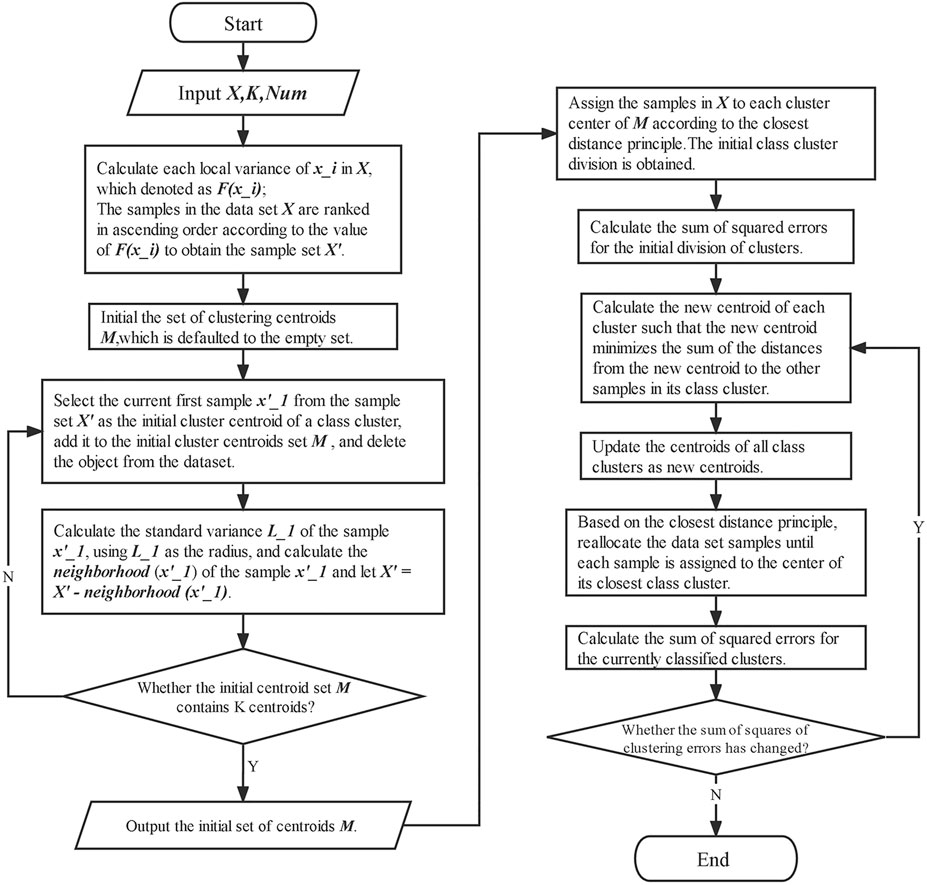
FIGURE 1. Flow of Num-near neighborhood K-medoids clustering based on local variance.

In this improved K-medoids clustering, the data sample set X, cluster number K, and Num should be input, and it outputs K clusters with finished clustering results when the iteration is stopped.

2.4 Improved spectral clustering

As mentioned previously, spectral clustering algorithms based on K-medoids and improved K-medoids (num-near neighbor K-medoids based on local variances) can be proposed, and the latter is highlighted here: when $M\times N$ samples are input, the affinity matrix is calculated based on formula 1, then the degree matrix is calculated based on formula 2; for a certain K-classification pattern recognition, formulas 3,4 accept the affinity matrix and degree matrix to output the corresponding Laplacian and normalized Laplacian matrices, then the algorithm intercepts the first K columns of the normalized Laplacian matrix by column $M\times K$ size $\left(K<N\right)$ and puts the intercepted matrix into the num-near neighbor K-medoids based on local variances, and outputs the clustering results. It is worth noting that the only difference between the spectral clustering algorithms based on K-medoids and improved K-medoids is the last step.

The two flows of the improved spectral clustering algorithms compared to the original NJW spectral clustering can be expressed as follows:

5.1, 5.2, and 5.3 represent three different clustering strategies of spectral clustering based on the original or proposed clustering algorithms in the last step of the flows; for the three flows, they share the common first four steps. As the upper-right subfigure in Figure 2 shows, the theoretical improvement in performance is dependent on the noise immunity of different clustering algorithms.

FIGURE 2

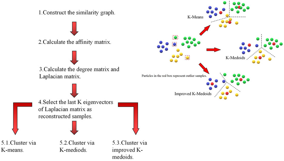
FIGURE 2. Comparison of proposed spectral clustering flows and original spectral clustering flow.

Considering that each step of the spectral clustering algorithms is independent of each other, there is a brief discussion about the time complexity of the three spectral clustering algorithms: for the original spectral clustering, the time complexity of the latter clustering (K-means) is $O\left(NKT\right)$, N is the size of the input samples, and T is the value of iterations; when the latter clustering follows step 5.2 (K-medoids), the single time complexity is $O\left(K{\left(N-K\right)}^2\right)$, and the time complexity of the latter clustering following step 5.3 (improved K-medoids) is $O\left(N^2+NKT\right)$ , because it comprises generating or adjusting the centroid set and calculating the distance between each sample and centroid on a more complex level. However, when it comes to workflow, the global time complexity is determined by the most complex procedure, while the time complexity of calculating the affinity matrix is $O\left(N^2\right)$, which contributes to the highest time complexity in the common part. Therefore, the global time complexities of the three spectral clustering are: $O\left(N^2\right)$ for original spectral clustering, $O\left(N^2\right)$ for spectral clustering based on K-medoids, and $O\left(N^2+NKT\right)$ for spectral clustering based on improved K-medoids. It is obvious that spectral clustering based on improved K-medoids is slightly more time-consuming than the other two, while it is acceptable when the targeted value of clusters is small.

2.5 Prediction for new samples

As unsupervised machine learning algorithms have label-independent features, clustering algorithms are often not applied to classification because there is no specifically defined clustering information at the end, which restricts their application in classification. However, semi-supervised learning strategies can construct connections between unlabeled and labeled samples to expand the availability of raw data without known features, and the original unsupervised learning flows can fit with the task of classification by labeling samples that have no semantic definitions.

Semi-supervised methodologies and algorithms, which are also based on the graph theory, can offer some inspiration and guidance regarding the intensity prediction of new rockburst samples in this research (Luxburg, 2007). A label propagation mechanism and algorithm developed from it can solve the task of labeling the remaining samples based on limited label information and the construction of an affiliation matrix that represents the connectional strength between each sample, which is similar to the spectral transformation process. The direct labeling process relies on the label propagation matrix $S$, which can be written as

$\mathit{S}={\mathit{D}}^{-\frac{1}{2}}\mathit{W}{\mathit{D}}^{-\frac{1}{2}},(12)$

where $D$ is also the degree matrix as in the previous definition.

The set of $\left(l+u\right)\times d$ nonnegative matrices named $F\left(t\right)$are defined, which represents that for a certain iteration $t$, there is one matrix describing the classification result for $l$ labeled samples and $u$ unlabeled samples. $F{\left(t\right)}_{ij}$ represents unlabeled sample $i$ $\left(l<i<l+u\right)$, which describes how close it belongs to classification $j$, and the maximum scale in row $i$ corresponds to the most possible classification of unlabeled sample $i$, which is the core mechanism of graph semi-supervised clustering. The initial matrix and iterative equation of $F$ can be written as

$\mathit{F}\left(\mathbf{0}\right)=\{\begin{array}{c}\mathbf{1}, \mathbf{i}\mathbf{f}\left(\mathbf{1}\le \mathit{i}\le l\right){{\displaystyle \cap }}^{\text{}}\left({\mathit{F}}_{\mathit{i}}\left(\mathbf{0}\right)=\mathit{j}\right)\\ \mathbf{0}, otherwise\end{array},(13)$

$\mathit{F}\left(\mathit{t}+\mathbf{1}\right)=\mathit{\alpha SF}\left(\mathit{t}\right)+\left(\mathbf{1}-\mathit{\alpha }\right)\mathit{F}\left(0\right),(14)$

The convergence state of $F$ can be written as

${\mathit{F}}^{\ast }=\underset{\mathit{t}\to \infty }{\mathbf{lim}}\mathit{F}\left(\mathit{t}\right)=\left(\mathbf{1}-\mathit{\alpha }\right){\left(\mathit{I}-\mathit{\alpha S}\right)}^{-\mathbf{1}}\mathit{F}\left(\mathbf{0}\right),(15)$

During each iteration, every sample receives effective information from its neighbors (first term) and retains its initial information (second term). a represents the harmonization factor of the neighborhood information for each sample. In fact, this information exchange mechanism is based on two prior assumptions of consistency: 1) nearby samples are likely to belong to the same label and 2) samples located on the same structure (typically in the same cluster or manifold) are likely to belong to the same label. It is worth noting that the former is based on local distribution, whereas the latter is a global assumption, and the convergence of $F$ is its implementation process. However, the spectral method does not require global information to achieve or reach a global stable state when processing the limited size of samples mixed into the original structure. In particular, all samples come from similar experiments and obey a similar distribution, which is different from the original motivation of semi-supervised clustering based on the graph theory. Furthermore, the complexity of labeling using this algorithm is $O\left({\left(l+u\right)}^2\right)$ , whereas the labels of most samples are known, which causes redundant expenses.

Therefore, it is feasible and necessary to propose a concise flow to meet the compact demand for labeling a few samples based on sufficient and homologous labeled samples. According to the aforementioned local hypothesis, measuring distances between unknown points and points that have label information (centroids determined in previous studies) is the most direct way to compare the similarity and match classifications under similar a spectral processing space (as shown in Figure 3). However, the influence of inputting new samples can be reduced by the robustness of the structure (based on the latter global hypothesis), maintaining the original structure by controlling the size and ensuring the homology of inputted unlabeled samples as far as possible.

FIGURE 3

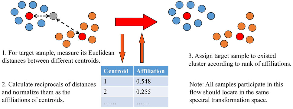
FIGURE 3. Flow of proposed concise labeling method for new samples.

In this study, a classification flow based on clustering and the original clustering results was proposed (as shown in Figure 4). Once the most successful configuration of the hyperparameters and clustering method was determined, it was selected as the backbone of the flow to classify the rockburst intensity of the new samples. In the classification phase, the new samples are mixed with the labeled samples (which are used in the previous clustering to obtain the configuration) before being placed into the clustering process, and the size of the new samples should be limited to a relatively lower level than the original samples, and clustering is executed, and whether clustering is successful. The criterion of success is that four intensity labels correspond to the four clusters one by one, and each statistical mode of the four types of labeled samples belongs to only one cluster. The cluster types are defined according to the degree of intensity when clustering is successful. The Euclidean distances between new samples and the four cluster centroids are calculated, and the reciprocals of distances are normalized as affiliations of each new sample to judge the intensity grade of every rockburst data.

FIGURE 4

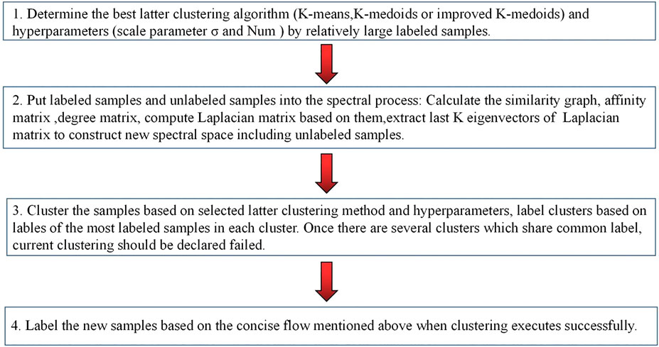
FIGURE 4. Flow of predicting new unlabeled samples based on spectral clustering algorithms.

Although the robustness of the space structure and multiple mechanisms can maintain stability during the process of expanding the dataset, too many additional samples can disturb or even destroy the benign distribution of original samples. Therefore, the size of the new samples should be limited. The latter additional samples do not participate in constructing semantic concepts, which should be noted. The full flow of predicting new unlabeled samples based on the spectral clustering algorithms used in the subsequent sections is as follows:

2.6 Rockburst mechanism analysis

After a long period of effort, a series of important results have been achieved in the field of rockburst research to eliminate the effects of underground construction as far as possible; however, to date, studies on the rockburst mechanism have not yet made a major breakthrough, that is, they have not been able to obtain a uniform, comprehensive, and reasonable theoretical explanation of the various types of rockburst phenomena that occur in different projects. Therefore, a reasonable comprehensive discussion based on different theories is necessary, and integrating sufficient indicators from the perspective of several theoretical criteria can avoid biased characterization and mapping of the causal relationship as much as possible.

The clearest overview of the rockburst mechanism thus far is that rockburst requires the presence of two conditions: the presence of a high-energy storage body, and its stress close to the strength of the rock is the endogenous cause of the rockburst; some additional load is triggered by the external cause of its generation (Zhou et al., 2018). Another explanation for this mechanism is that in the structure of intact hard brittle surrounding rock under high ground stress conditions, after tunnel excavation, the shear stress reaches or approaches the uniaxial compressive strength of the surrounding rock. Induced by other factors, the surrounding rock would be destabilized in the form of a rockburst, which can be summarized as a rockburst formation mechanism of the static load (hydrostatic) theory.

The rock-static theory is important in the study of rockbursts, but it cannot clarify the full mechanism of rockbursts. The initial ground stress and excavation-induced stress divergence are the background and basis for the occurrence of rockbursts, but not all; there should be other triggering mechanisms outside geostatic stress. The energy theory is commonly used as a supplement to predict rockburst intensity and is based on the relationship between the damage characteristics and energy change in the process of deformation of the surrounding rock (Zhou et al., 2018). Wang and Park (2001) pointed out that two main factors play the most important role in the occurrence of rockbursts: the property of storing strain energy in the rock mass and the distributional situation of stress concentration and energy accumulation.

For hard surrounding rocks in high ground stress areas, the brittleness theory may be more reasonable for explaining the cause of rockburst (Gong et al., 2020), which considers that rockburst is a violent release of elastic strain energy reserves of hard brittle rock due to excavation or other disturbances, leading to ground stress divergence, surrounding rock stress jump, and further concentration of energy, ultimately causing tension-shear brittle damage.

Combining all the mentioned generating mechanisms of rockburst, further discussion on rockburst judgment indicator sets will be executed in the next section; a relatively comprehensive and well-considered indicator set could have a more compatible ability to analyze various types of rockbursts caused by different trigger mechanisms, which should be proposed based on the commonly used criteria of every theory.

2.7 Indicator analysis and selection

A rockburst is a complex nonlinear dynamic phenomenon that combines several theoretical criteria and methods to accurately evaluate its intensity (Wang et al., 2019). Lithology-based rockburst index attributions are the most widely used discrimination criteria in rockburst intensity prediction, which mainly include stress/strength-based index attributions, energy-based attributions, and brittleness index attributions. Based on this index framework, further exploration and selection of specific attributions used to predict the intensity are discussed.

The establishment of stress attributions is based on the strength theory. The strength theory is generally based on the strength of the rock as a metric, from the static equilibrium conditions of the surrounding rock, and various stress intensity guidelines as one of the criteria for rockbursts. The strength theory is often based on uniaxial test results derived from this basis, which cannot accurately explain the ejection mechanism of a rock mass (piece); however, its concept is clear, concise, and practical, so it has been more widely used. Uniaxial compressive strength (UCS, which is also denoted as ${\sigma }_c$) and maximum tangential stress (MTS, which is also denoted as ${\sigma }_{\theta }$) around the tunnel are the most direct and basic index attributes used in many stress-based evaluation criteria, such as the Turchaninov criterion, Russenes’ criterion, and Hoek criterion, which reflect the levels of load and resistance to the accumulated load. Uniaxial tensile strength (UTS, or ${\sigma }_t$) is another indicator commonly used in the criteria of intensity classification, and should also be considered as an evaluation attribute in datasets. It is worth noting that all three attributes or indicators can be obtained from the uniaxial compression test.

The elastic strain energy storage index $W_{et}$ is another indicator obtained from the uniaxial compression test, and its physical meaning is the ratio of the elastic strain energy accumulated to dissipated in the tested samples, which represents the tolerance and current situation of the strain energy. According to the energy-based criterion, when the rock mass-surrounding rock system is in a state of mechanical equilibrium disruption, the energy released by the system is greater than the energy consumed, that is, the rockburst. The elastic strain energy accumulated in the rock is the dominant internal factor in the occurrence of rockbursts, which better explains the energy source of rockbursts and the dynamic phenomena in rockbursts, such as earthquakes and rock ejection.

According to the brittleness index criterion, rockburst is the brittle destruction of rock mass. So, establishing brittleness index indicators to evaluate the intensity of the rockburst is feasible and necessary; the commonly used indicators are the stress concentration factor (SCF) and two types of brittleness indexes, that is, $B_1$ and $B_2$, the former was proposed by Zhu et al. (1996) and the latter was proposed by Singh (1987), and they are noted as

$\mathit{SCF}=\frac{{\mathit{\sigma }}_{\mathit{\theta }}}{{\mathit{\sigma }}_{\mathit{c}}},(16)$

${\mathit{B}}_{\mathbf{1}}=\frac{{\mathit{\sigma }}_{\mathit{c}}}{{\mathit{\sigma }}_{\mathit{t}}},(17)$

${\mathit{B}}_{\mathbf{2}}=\frac{{\mathit{\sigma }}_{\mathit{c}}-{\mathit{\sigma }}_{\mathit{t}}}{{\mathit{\sigma }}_{\mathit{c}}+{\mathit{\sigma }}_{\mathit{t}}},(18)$

All brittleness index indicators rely on the stress index attributes mentioned previously, whereas these index indicators include the potential mechanical properties of rock that would not be recognized by the indirect pattern recognition algorithm.

Seven indicators were selected for this study: UCS $\left({\sigma }_c\right)$, MTS $\left({\sigma }_{\theta }\right)$, UTS $\left({\sigma }_t\right)$, $W_{et}$, SCF, $B_1$, and $B_2$. These indicators are commonly used as feasible parameters for evaluating the rockburst intensity.

2.8 Intensity degree

To better describe the difference in intensities and rockburst phenomena, rockbursts tend to be classified into four degrees: none (N), light (L), moderate (M), and high (H). While there are several criteria to classify rockburst datasets, different classification results would correspond to a certain sample. The commonly used classification criteria for rockburst intensity levels have a high degree of validity; however, it is important to note that all samples must be evaluated under the same classification framework and intensity degree criterion. In this study, the classification proposed by Zhou et al. (2012) was considered the unique intensity degree criterion (as shown in Table 1).

TABLE 1

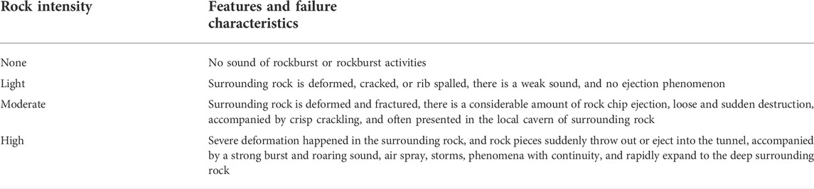
TABLE 1. Classification criterion for rockburst intensity proposed by Zhou et al. (2012).

2.9 Distribution of selected samples

According to the aforementioned classification criteria of intensity degrees and indicators, the dataset extracted from Zhou et al. (2016), and 82 samples collected from engineering practices in the dataset were further selected; 65 samples in the selected set were selected as the “seed samples” to construct the clusters, determine the hyperparameters, and train supervised algorithms in the control group, while the remaining 17 samples were only used to play the role of a benchmark in final comparisons. It is worth noting that all the samples came from several uniform experiments and obey the same distributional pattern as far as possible.

There were 16 samples in degree N, 20 samples in degree L, 15 samples in degree M, and 14 samples in degree H, indicating a relatively uniform distribution. It is worth noting that except $W_{et}$ in degree H, all the indicators at 4° show a nonlinear and almost non-convex distribution pattern, which represents a challenge to the spectral clustering algorithms mentioned and other supervised learning algorithms.

2.10 Performance measure

In this study, accuracy was selected as the main evaluation indicator, and comparison and reference standards are generally sufficient for evaluating the performance of multi-class tasks; however, more indicators should be considered in certain processes. To describe and evaluate the clustering and classification results more comprehensively, the measure indices marco-P, marco-R, and marco-F1 were introduced, and they can be presented as follows:

${\mathit{P}}_{\mathit{i}}=\frac{\mathit{T}{\mathit{P}}_{\mathit{i}}}{\mathit{T}{\mathit{P}}_{\mathit{i}}+\mathit{F}{\mathit{P}}_{\mathit{i}}},(19)$

${\mathit{R}}_{\mathit{i}}=\frac{\mathit{T}{\mathit{P}}_{\mathit{i}}}{\mathit{T}{\mathit{P}}_{\mathit{i}}+\mathit{F}{\mathit{N}}_{\mathit{i}}}(20)$

$\mathbf{m}\mathbf{a}\mathbf{r}\mathbf{c}\mathbf{o}-\mathit{P}=\frac{1}{\mathit{n}}{\sum }_{\mathit{i}=1}^{\mathit{n}}{\mathit{P}}_{\mathit{i}},(21)$

$\mathbf{m}\mathbf{a}\mathbf{r}\mathbf{c}\mathbf{o}-\mathit{R}=\frac{1}{\mathit{n}}{\sum }_{\mathit{i}=1}^{\mathit{n}}{\mathit{R}}_{\mathit{i}},(22)$

$\mathbf{m}\mathbf{a}\mathbf{r}\mathbf{c}\mathbf{o}-\mathit{F}1=\frac{2\times \mathbf{m}\mathbf{a}\mathbf{r}\mathbf{c}\mathbf{o}-\mathit{P}\times \mathbf{m}\mathbf{a}\mathbf{r}\mathbf{c}\mathbf{o}-\mathit{R}}{\mathbf{m}\mathbf{a}\mathbf{r}\mathbf{c}\mathbf{o}-\mathit{P}+\mathbf{m}\mathbf{a}\mathbf{r}\mathbf{c}\mathbf{o}-\mathit{R}},(23)$

where $T{P}_i$ represents the true positive samples classified in cluster $i$, which defines the cluster’s corresponding intensity label according to most samples with the same intensity degree falling into the cluster in this study. $F{P}_i$ and $F{N}_i$ are false-positive and false-negative results, respectively. In this study, cluster numbers n=4, which are counterparts to the four degrees of rockburst. $P_i$ and $R_i$ are the precision and recall, respectively, of cluster $i$. To describe the general performance of the clustering results, marco-P and marco-R represent the arithmetic averages of $P$ and $R$ of all clusters, respectively; therefore, the harmonic mean of both would offer a more comprehensive consideration of the performance of every algorithm, which leads to the introduction of marco-F1 as a performance measure.

3 Result and discussion

3.1 Experimental setup

All experiments in this study were implemented using MATLAB R2021a with the following specifications: AMD Ryzen 7 4800H with Radeon Graphics 2.90 GHz., RAM of 16 GB RAM, and Windows 10 H.20 64bit.

3.2 Determination of parameters configuration

There are two types of hyperparameters in this study: the scale parameter σ and the near neighbor parameter Num, where σ determines the similarity between pairs of data points and is reflected in the affinity matrix when the similarity is calculated using a Gaussian function. The physical meaning of σ can be described as controlling the decay rate of distances. If the value of σ is too small, all weights in the matrix converge to zero and all points remain far from each other. In contrast, too large a value of σ would lead weights to converge to 1, which makes all the points equally close. In both situations, the distance between each pair of points cannot be accurately defined (Favati et al., 2020). Therefore, σ must be determined using several control experiments.

When it comes to the selection of the near-neighbor parameter Num, it is worth noting that because of the different distribution of samples in the dataset, when different Num values are taken, the neighborhood range sizes are different, and the obtained local variances would fluctuate. A reasonable Num value would generate better initial cluster centroids and, thus, a better clustering result.

Because two hyperparameters appear in different phases of spectral clustering algorithms, and only spectral clustering based on improved K-medoids uses Num to control the generation of initial centroids, while σ determines the decay rate of distance in the weight measure in all spectral transformation processes, the sequence of determination should be considered. The NJW algorithm performs spectral clustering by specifying several values of the scale parameter σ in advance, and finally selects the σ that performs the best clustering result as the parameter, which eliminates the subjective influences of the scale parameter selection; generally, the range of selection is 0.1–10. To avoid redundant computational expenses, the strategy of selecting values at certain intervals was adopted in all control experiments related to σ.

The first hypermeter determined and optimized was Num in near-neighbor K-medoids, according to the experimental results shown in Xie and Gao (2015); there are several values of Num corresponding to relatively perfect clustering accuracy in various datasets such as IRIS, Soybean, and Wine. In the 65 sample-size experiments, the feasible values of Num were integers between 1 and 65. Because the most appropriate σ had not been found in this phase, a smaller interval and larger search range were selected in the trial-and-error search process: setting 0.05 as the minimum interval, the initial value is 0.75 and the end value is 2.0, while the extreme values are 0.5 and 1.4 in the next experiment for the determinations of σ and best latter clustering process. To refine the length of this study, only the curves for several σ values are shown.

As shown in Figure 5, it appears that there are also several points or even continuous intervals corresponding to the most accurate results for all curves. In fact, many Nums maintain the same level of accuracy, which means that fluctuations of results with the change in Num are slight or even do not exist when the curves are horizontal. With increasing σ, this effect becomes more obvious, whereas the best accuracy rates decrease. Two preliminary conclusions were drawn: 1. It is feasible to find one universal value of the near-neighbor parameter for 65 samples and other different hypermeters. 2. The appropriate scale parameters are located in the selected intervals and should be experimented with and further discussed in the next section.

FIGURE 5

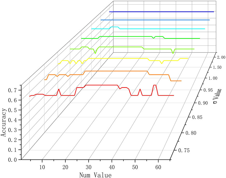
FIGURE 5. Accuracy under different Num values and σ values.

Considering all eight conditions corresponding to different scale parameters, it is not difficult to find that nearly all of the most accurate performances correspond to intervals that contain the sub-range, which is 26–40, and each condition would reach the highest point when Num is 30. Further analysis can be obtained from the mechanisms and formulas of near neighbors based on local variance: once Num is too small, only local near samples can be marked as a near neighbor for a certain point, and the near-neighbor set does not include sufficient information about global features of the distribution, which is adverse for the generation of initial centroids. When Num is too large, the outlier points are incorporated into the neighbor and disturb the calculation result of the local variance to a certain extent, even if the local variance mechanism is noise-proof. In summary, selecting 30 as the value of Num would fit with the near-neighbor K-medoids, which is set as the latter clustering process in the improved spectral clustering in this dataset, which is used in rockburst intensity classification.

There were 19 control groups in the determination of σ that compared the three spectral clustering algorithms with different clustering processes: K-means, K-medoids, and improved K-medoids with Num=30.

It is worth noting that the confusion matrices of the four clusters are the original sources of the measurement calculation, which are based on the definition of the cluster labels. The performance measurement curves can be expressed as Figure 6 shows:

FIGURE 6

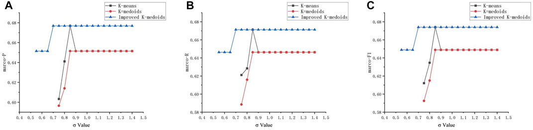
FIGURE 6. Performance measures of three latter clustering algorithms in different scale parameters σ(A) marco-P; (B) marco-R; and (C) marco-F1.

Obviously, the spectral clustering that uses the proposed improved K-medoids outputs more accurate clustering results compared to the other two under the same scale parameter; the success rate of the proposed improved flow is also higher; once two or more clusters obtain the same label, the flow will stop and return an error, current clustering is declared failed, which is a difficult strategy compared to other soft classification strategies (Chen et al., 2021), which is also the reason why some points are missed in the aforementioned figure. In fact, most confusion matrices of failed clustering results show that there is some difficulty in the effective discrimination of samples under light (L) and moderate (M) conditions, which is also an issue in other rockburst intensity prediction methods. The influence of variation in σ can be described as follows: the probability of success and rate of accuracy increase with an increase in σ, while there are limitations for all clustering results, so excessively large values of σ cannot enhance the performance of clustering. In summary, when σ is 0.85, it is more credible that all the latter clustering processes, including the improved K-medoids, can achieve the best performance.

Finally, the improved K-medoids were justified as the best replacement for the original K-means process of traditional spectral clustering in this research; Num=30 and σ=0.85 were selected as the optimized configurations of the hyperparameters used in the next section.

3.3 Comparison of five algorithms

In this section, the classification performance of the improved spectral clustering approach is discussed and compared with that of the other four machine learning algorithms using selected rockburst intensity datasets. The 65 samples (as shown in Table 3) used to determine the best spectral clustering flow and hyperparameters were selected as the training and validation data for the other algorithms, and 17 samples were selected to construct the common test set.

The algorithms in the control group were all supervised learning algorithms: artificial neural network (ANN), support vector machine (SVM), linear discriminant analysis (LDA), and Gaussian process classification (GPC); 8-fold cross-validation was selected as the training and validation set partitioning strategy for all control algorithms.

Based on the size of the input indicators and classification results (rockburst intensity degrees), the backpropagation network part was set to 7–10–4 (7 units in the input layer, 10 units in the hidden layer, and 4 units in the output layer). The hyperparameters of the network were determined as follows: the activation function was ReLU and the maximum iteration time was 1,000.

In this control experiment, a multi-classification support vector machine classification model incorporating a multiclass error correction output coding (ECOC) strategy was used, and the kernel function was a radial basis function (RBF).

In LDA classification, the normal covariance structure was replaced by a diagonal covariance structure to eliminate the effect of singular covariance matrices.

The GPC model used in this control group is based on the softmax curve as the function corresponding to the multi-classification task.

Only accuracy was selected as the indicator to measure and compare the algorithms mentioned, which should consider the performance on the validation sets (65 samples) and test sets (17 samples) to judge whether better generalization performance has been obtained for each algorithm.

From Figure 7 and Table 2, it is obvious that the proposed spectral clustering method may not have the best accuracy compared to other algorithms on the validation set, whereas it predicted nearly all the intensity degrees of the test samples successfully, indicating that the proposed method has better generalization performance and is more significant for engineering applications. Further analysis and discussion based on restrictions or hypotheses are presented in the Discussion section (Section 5). To facilitate the reader to conduct control experiments on other classification algorithms, the full sample of the training set used in this study is published here, which was extracted from the study mentioned previously (Zhou et al., 2016).

FIGURE 7

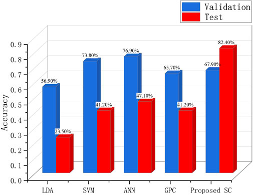
FIGURE 7. Comparisons of five algorithms in the validation set and the test set.

TABLE 2

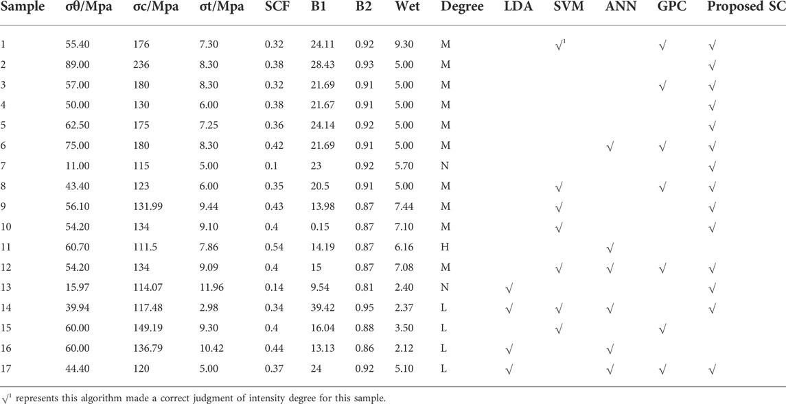
TABLE 2. Seventeen test samples and judgments of each algorithm.

TABLE 3

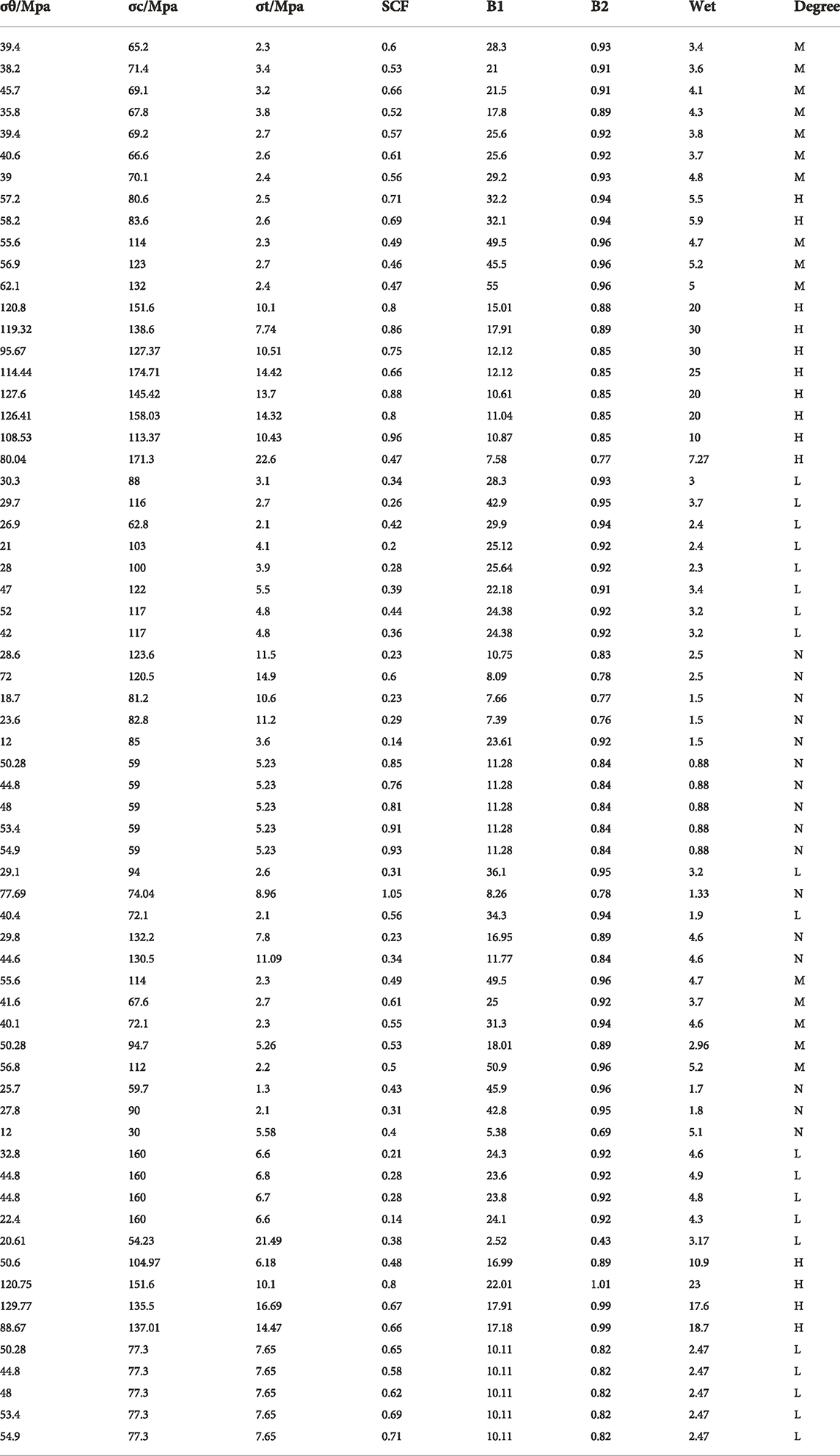
TABLE 3. Set of training samples used in this study.

3.4 Discussion

The results shown as follows indicate that it is feasible to predict the intensity degrees of rockbursts for rock samples in underground buildings and tunnels based on the spectral clustering algorithm. Relatively ideal prediction results can be obtained by appropriate improvements and expanding flows, although there are several problems that should be considered.

In this study, sufficient research and a reasonable selection of indicators that play the role of input parameters in clustering or other learning models are considered, which is significant for ensuring the reliability and reasonability of data-driven methods. The absence of intermediate process demonstration in models is a common problem in the application of nearly all data-driven methods, including machine learning techniques, to rockburst intensity prediction; therefore, refining input parameters is one of the most effective measures to control the quality of information outputted by target models, which would guide model prediction in logical ways and enhance interpretability for prediction results.

When it comes to spectral clustering, optimization from the perspective of the latter clustering method (K-means used in the original flow) is the easiest way to achieve; K-medoids and improved K-medoids were considered, which caused the problems and discussions on hyperparameters: improved K-medoids should consider near neighborhood parameter Num, while the mechanism of how Num influences the final clustering results has still not been clarified in previous research (Xie and Gao, 2015), so it is inevitable to search for hyperparameters via a fully covered trial-and-error experiment.

The expanding flow of labeling new samples based on previous works and the labeled samples proposed in this study is a supplementary measure that empowers spectral clustering algorithms to label and classify samples, which is beyond the ability of traditional clustering algorithms. This is based on the hypothesis of sample distribution in the semi-supervised learning process, which is also based on the graph theory, and obtained relatively ideal results in the prediction of unlabeled samples (82.40% in the performance of accuracy). Stricter mathematical deduction and proof of whether the consistency of samples can maintain the consistency of clusters in two phases should be explored in future studies.

4 Conclusion

In this study, an improved spectral clustering algorithm was proposed for rockburst intensity classification and prediction. First, K-medoids and optimized K-medoids by the variance of the Num-near neighbor were introduced to the traditional NJW spectral clustering to replace K-means as the latter direct clustering process, and the improved K-medoids were selected because of their high accuracy and rate of success. The best configuration of hyperparameters for improved K-medoids was determined for the selected rockburst intensity samples, which were also the training sets of supervised learning algorithms in the control group. Finally, based on the labeled datasets used in the previous process, improved spectral clustering predicted the rockburst intensity degrees of new unlabeled samples by constructing and labeling clusters according to the labeled datasets, and the affiliations to four degrees of each new sample were the judgment criteria of rockburst intensity. Compared with other machine learning algorithms used to classify intensity, the accuracy and stability of the proposed improved spectral clustering were verified. It should be noted that appropriate hyperparameters and feasible data samples are the key elements for achieving successful clustering and classification.

Although the satisfactory performance of the improved algorithm and method was observed, no implicit information between the indicators and intensity distributions was found via the flow, which failed to fully exploit the advantages of unsupervised learning. Strict mathematical discussion and deduction of the interference of the new sample with the original sample space are insufficient. The success criterion for clustering is too difficult to always obtain ideal clusters, and adopting a soft category mechanism may be an effective measure to avoid this unfavorable situation. As a data-driven method, the proposed algorithm is advised to be used as a component in ensemble learning machines for rockburst intensity prediction in early warnings for tunnels or other underground buildings to ensure more accurate and credible results.

Data availability statement

Publicly available datasets were analyzed in this study. These data can be found at: https://doi.org/10.1061/(ASCE)CP.1943–5487.0000553.

Author contributions

ZX contributed to conception and design of the study. ZX and YH organized the databases. ZX and YH performed the statistical analysis. ZX and JM wrote the first draft of the manuscript. ZX and JM wrote sections of the manuscript. All authors contributed to manuscript revision, read, and approved the submitted version.

Acknowledgments

The contribution of each participant to the research work corresponding to this article is significant and not negligible, for which we express our sincere gratitude.

Conflict of interest

The authors declare that the research was conducted in the absence of any commercial or financial relationships that could be construed as potential conflicts of interest.

Publisher’s note

All claims expressed in this article are solely those of the authors and do not necessarily represent those of their affiliated organizations, or those of the publisher, the editors, and the reviewers. Any product that may be evaluated in this article, or claim that may be made by its manufacturer, is not guaranteed or endorsed by the publisher.

References

Adoko, A. C., Gokceoglu, C., Wu, L., and Zuo, Q. J. (2013). Knowledge-based and data-driven fuzzy modeling for rockburst prediction. Int. J. Rock Mech. Min. Sci. (1997). 61, 86–95. doi:10.1016/j.ijrmms.2013.02.010

CrossRef Full Text | Google Scholar

Bai, L., Zhao, X., Kong, Y., Zhang, Z., Shao, J., and Qian, Y. (2021). Survey of spectral clustering algorithms. Comput. Eng. Appl. 57, 12. doi:10.3778/j.issn.1002-8331.2103-0547

CrossRef Full Text | Google Scholar

Chen, G., Wang, M., Yan, J., and Shen, F. (2021). A connection cloud model coupled with improved conflict evidence fusion method for prediction of rockburst intensity. IEEE Access 9, 113535–113549. doi:10.1109/ACCESS.2021.3102330

CrossRef Full Text | Google Scholar

Dong, L.-J., Li, X.-B., and Kang, P. (2013). Prediction of rockburst classification using Random Forest. Trans. Nonferrous Metals Soc. China 23, 472–477. doi:10.1016/S1003-6326(13)62487-5

CrossRef Full Text | Google Scholar

Favati, P., Lotti, G., Menchi, O., and Romani, F. (2020). Construction of the similarity matrix for the spectral clustering method: Numerical experiments. J. Comput. Appl. Math. 375, 112795. doi:10.1016/j.cam.2020.112795

CrossRef Full Text | Google Scholar

Ge, J., and Yang, G. (2021). Spectral clustering algorithm for density adaptive neighborhood based onshared nearest neighbors. Comput. Eng. 47, 8. doi:10.19678/j.issn.1000-3428.0058893

CrossRef Full Text | Google Scholar

Ghasemi, E., Gholizadeh, H., and Adoko, A. C. (2020). Evaluation of rockburst occurrence and intensity in underground structures using decision tree approach. Eng. Comput. 36, 213–225. doi:10.1007/s00366-018-00695-9

CrossRef Full Text | Google Scholar

Gong, F.-Q., Luo, Y., Li, X.-B., Si, X.-F., and Tao, M. (2018). Experimental simulation investigation on rockburst induced by spalling failure in deep circular tunnels. Tunn. Undergr. Space Technol. 81, 413–427. doi:10.1016/j.tust.2018.07.035

CrossRef Full Text | Google Scholar

Gong, F.-Q., Wang, Y.-L., and Luo, S. (2020). Rockburst proneness criteria for rock materials: Review and new insights. J. Cent. South Univ. 27, 2793–2821. doi:10.1007/s11771-020-4511-y

CrossRef Full Text | Google Scholar

Guo, J., Wang, S., and Xu, Q. (2022). Saliency guided DNL-yolo for optical remote sensing images for off-shore ship detection. Appl. Sci. (Basel). 12, 2629. doi:10.3390/app12052629

CrossRef Full Text | Google Scholar

He, S., Song, D., Mitri, H., He, X., Chen, J., Li, Z., et al. (2021). Integrated rockburst early warning model based on fuzzy comprehensive evaluation method. Int. J. Rock Mech. Min. Sci. (1997). 142, 104767. doi:10.1016/j.ijrmms.2021.104767

CrossRef Full Text | Google Scholar

Li, D., Liu, Z., Armaghani, D. J., Xiao, P., and Zhou, J. (2022). Novel ensemble intelligence methodologies for rockburst assessment in complex and variable environments. Sci. Rep. 12, 1844. doi:10.1038/s41598-022-05594-0

PubMed Abstract | CrossRef Full Text | Google Scholar

Li, Y., Yuan, Y.-H., and Zhao, X.-M. (2018). Spectral clustering of variable class for remote sensing image segmentation. Acta Elect. Sini 46, 8. doi:10.3969/j.issn.0372-2112.2018.12.028

CrossRef Full Text | Google Scholar

Liang, W., Sari, A., Zhao, G., Mckinnon, S. D., and Wu, H. (2020). Short-term rockburst risk prediction using ensemble learning methods. Nat. Hazards (Dordr). 104, 1923–1946. doi:10.1007/s11069-020-04255-7

CrossRef Full Text | Google Scholar

Liang, W., Zhao, G., Wu, H., and Dai, B. (2019). Risk assessment of rockburst via an extended MABAC method under fuzzy environment. Tunn. Undergr. Space Technol. 83, 533–544. doi:10.1016/j.tust.2018.09.037

CrossRef Full Text | Google Scholar

Luxburg, U. V. (2007). A tutorial on spectral clustering. Stat. Comput. 17, 395–416. doi:10.1007/s11222-007-9033-z

CrossRef Full Text | Google Scholar

Ma, T.-H., Tang, C.-A., Tang, S.-B., Kuang, L., Yu, Q., Kong, D.-Q., et al. (2018). Rockburst mechanism and prediction based on microseismic monitoring. Int. J. Rock Mech. Min. Sci. (1997). 110, 177–188. doi:10.1016/j.ijrmms.2018.07.016

CrossRef Full Text | Google Scholar

Pellicer-Valero, O. J., FERNáNDEZ-de-Las-PEñAS, C., MARTíN-Guerrero, J. D., Navarro-Pardo, E., CIGARáN-MéNDEZ, M. I., Florencio, L. L., et al. (2020). Patient profiling based on spectral clustering for an enhanced classification of patients with tension-type headache. Appl. Sci. (Basel). 10, 9109. doi:10.3390/app10249109

CrossRef Full Text | Google Scholar

Pu, Y., Apel, D. B., and Xu, H. (2019). Rockburst prediction in kimberlite with unsupervised learning method and support vector classifier. Tunn. Undergr. Space Technol. 90, 12–18. doi:10.1016/j.tust.2019.04.019

CrossRef Full Text | Google Scholar

Rebagliati, N., and Verri, A. (2011). Spectral clustering with more than K eigenvectors. Neurocomputing 74, 1391–1401. doi:10.1016/j.neucom.2010.12.008

CrossRef Full Text | Google Scholar

Shen, C., Qian, L., and Yu, N. (2021). Adaptive facial imagery clustering via spectral clustering and reinforcement learning. Appl. Sci. (Basel). 11, 8051. doi:10.3390/app11178051

CrossRef Full Text | Google Scholar

Shirani faradonbeh, R., Shaffiee Haghshenas, S., Taheri, A., and Mikaeil, R. (2020). Application of self-organizing map and fuzzy c-mean techniques for rockburst clustering in deep underground projects. Neural comput. Appl. 32, 8545–8559. doi:10.1007/s00521-019-04353-z

CrossRef Full Text | Google Scholar

Singh, S. (1987). The influence of rock properties on the occurrence and control of rockbursts. Min. Sci. Technol. 5, 11–18. doi:10.1016/S0167-9031(87)90854-1

CrossRef Full Text | Google Scholar

Sun, Y., Li, G., Zhang, J., and Huang, J. (2021). Rockburst intensity evaluation by a novel systematic and evolved approach: Machine learning booster and application. Bull. Eng. Geol. Environ. 80, 8385–8395. doi:10.1007/s10064-021-02460-7

CrossRef Full Text | Google Scholar

Wang, C., Wu, A., Lu, H., Bao, T., and Liu, X. (2015). Predicting rockburst tendency based on fuzzy matter–element model. Int. J. Rock Mech. Min. Sci. (1997). 75, 224–232. doi:10.1016/j.ijrmms.2015.02.004

CrossRef Full Text | Google Scholar

Wang, H., Nie, L., Xu, Y., Lv, Y., He, Y., du, C., et al. (2019). Comprehensive prediction and discriminant model for rockburst intensity based on improved variable fuzzy sets approach. Appl. Sci. (Basel). 9, 3173. doi:10.3390/app9153173

CrossRef Full Text | Google Scholar

Wang, J.-A., and Park, H. (2001). Comprehensive prediction of rockburst based on analysis of strain energy in rocks. Tunn. Undergr. Space Technol. 16, 49–57. doi:10.1016/S0886-7798(01)00030-X

CrossRef Full Text | Google Scholar

Wang, L., and Shi, J. (2021). A comprehensive application of machine learning techniques for short-term solar radiation prediction. Appl. Sci. (Basel). 11, 5808. doi:10.3390/app11135808

CrossRef Full Text | Google Scholar

Wen, Z., Wang, X., Tan, Y., Zhang, H., Huang, W., Li, Q., et al. (2016). A study of rockburst hazard evaluation method in coal mine. Shock Vib. 2016, 1. doi:10.1155/2016/8740868

CrossRef Full Text | Google Scholar

Wu, S., Wu, Z., and Zhang, C. (2019). Rock burst prediction probability model based on case analysis. Tunn. Undergr. Space Technol. 93, 103069. doi:10.1016/j.tust.2019.103069

CrossRef Full Text | Google Scholar

Xie, J.-Y., and Ding, L.-J. (2019). The true self-adaptive spectral clustering algorithms. Acta Elect. Sini 47, 9. doi:10.3969/j.issn.0372-2112.2019.05.004

CrossRef Full Text | Google Scholar

Xie, J.-Y., and Gao, R. (2015). Optimized K-medoids clustering algorithm by variance of Num-near neighbour. Appli Res. Comput. 32, 5. doi:10.3969/j.issn.1001-3695.2015.01.007

CrossRef Full Text | Google Scholar

Xie, X. B., and Pan, C. L. (2007). Rockburst prediction method based on grey whitenization weight function cluster theory. J. Hunan Univ. (N.S.) 34, 5. CNKI:SUN:HNDX.0.2007-08-005. doi:10.1007/s10870-007-9222-9

CrossRef Full Text | Google Scholar

Xu, J., Jiang, J., Xu, N., Liu, Q., and Gao, Y. (2017). A new energy index for evaluating the tendency of rockburst and its engineering application. Eng. Geol. 230, 46–54. doi:10.1016/j.enggeo.2017.09.015

CrossRef Full Text | Google Scholar

Xue, Y., Bai, C., Kong, F., Qiu, D., Li, L., Su, M., et al. (2020a). A two-step comprehensive evaluation model for rockburst prediction based on multiple empirical criteria. Eng. Geol. 268, 105515. doi:10.1016/j.enggeo.2020.105515

CrossRef Full Text | Google Scholar

Xue, Y., Bai, C., Qiu, D., Kong, F., and Li, Z. (2020b). Predicting rockburst with database using particle swarm optimization and extreme learning machine. Tunn. Undergr. Space Technol. 98, 103287. doi:10.1016/j.tust.2020.103287

CrossRef Full Text | Google Scholar

Yang, T., Zhu, H.-D., Ma, Y.-C., Wang, Y.-R., and Yang, X.-F. (2021). Semi-supervised spectral clustering algorithm based on L2, 1 norm and manifold regularization terms. J. ShanD Uni(N.S.) 56, 10. doi:10.6040/j.issn.1671-9352.4.2020.218

CrossRef Full Text | Google Scholar

Zhou, J., Li, X., and Hani S, M. (2016). Classification of rockburst in underground projects: Comparison of ten supervised learning methods. J. Comput. Civ. Eng. 30, 19. doi:10.1061/(ASCE)CP.1943-5487.0000553

CrossRef Full Text | Google Scholar

Zhou, J., Li, X., and Mitri, H. S. (2018). Evaluation method of rockburst: State-of-the-art literature review. Tunn. Undergr. Space Technol. 81, 632–659. doi:10.1016/j.tust.2018.08.029

CrossRef Full Text | Google Scholar

Zhou, J., Li, X., and Shi, X. (2012). Long-term prediction model of rockburst in underground openings using heuristic algorithms and support vector machines. Saf. Sci. 50, 629–644. doi:10.1016/j.ssci.2011.08.065

CrossRef Full Text | Google Scholar

Zhu, G.-H., Huang, S.-B., Yuan, C.-F., and Huang, Y.-H. (2018). SCoS: The design and implementation of parallel spectral clustering algorithm based on spark. Chin. J. Comput. 41, 18. doi:10.11897/SP.J.1016.2018.00868

CrossRef Full Text | Google Scholar

Zhu, P., Yuanhan, W., and Tingjie, L. (1996). Griffith theory and the criteria of rock burst. Chin.J. Rock Mech. Geotech. Eng. 15, 5.

Google Scholar

Zhu, W., Li, Z., Zhu, L.-K., and Tang, C. (2010). Numerical simulation on rockburst of underground opening triggered by dynamic disturbance. Tunn. Undergr. Space Technol. 25, 587–599. doi:10.1016/j.tust.2010.04.004

CrossRef Full Text | Google Scholar