 Christine E. Hatch
 Erika T. Ito
94% of researchers rate our articles as excellent or good
Learn more about the work of our research integrity team to safeguard the quality of each article we publish.
Find out more
ORIGINAL RESEARCH article
Front. Earth Sci., 05 October 2022
Sec. Hydrosphere
Volume 10 - 2022 | https://doi.org/10.3389/feart.2022.945065
This article is part of the Research TopicNovel Approaches for Understanding Groundwater Dependent Ecosystems in a Changing EnvironmentView all 6 articles
Freshwater wetlands are groundwater-dependent ecosystems that require groundwater for saturation, for wetland plants and creatures, for maintenance of wetland soils, and thermal buffering. With worldwide wetland area in decline for decades if not centuries, finding and restoring wetlands provides enormous ecosystem and public benefits, yet so often these projects fail to yield self-sustaining wetland ecosystems. One reason is that restored wetlands are often built in places that are neither wet enough nor possess the underlying geology to sustain them, and they dry out or require continual (expensive!) water inputs. Massachusetts is making the best of a challenging situation for the declining cranberry farming industry: while competition from less expensive land and more productive varietals shifts cranberry production to other locations, everything under historic cranberry farms is ripe for resilient wetland restoration projects. These low-lying water-rich areas are underlain by glacial geology (peats and clays) that are ideal for holding water, they possess historic seed banks of wetland plants and large accumulations of organic and hydric soils, and are currently sought-after by a statewide restoration program, for which these results provide critical information for restoration design, enabling practitioners to maximize the capture and residence time of groundwater inputs to sustain the future wetland. In this paper, we investigate the human legacy of cranberry farming on the surface of a wetland as it has created a unique hydrogeologic unit: the anthropogenic aquifer. Water moves through an anthropogenically constructed aquifer in specific and predictable ways that were engineered to favor a monoculture of cranberry plants on the surface of what once was a peatland. In order to restore this landscape to a functioning freshwater wetland, every property of the anthropogenic aquifer must be reversed. We detail observational, thermal, hydrologic, geologic and isotopic evidence for the location of groundwater inflows to Foothills Preserve in southeastern Massachusetts. The specific properties of the Anthropogenic aquifer, and the location and magnitude of groundwater discharge at this location provide crucial information for practitioners when designing plans for a self-sustaining, resilient restored freshwater wetland on this and future sites.
Evidence of human activities has been present on Earth’s surface as long as humans have inhabited it, but human land use practices over the last 200–300 years have yielded such an unprecedented, observable footprint, that scientists have given this time period the moniker The Anthropocene and included it in the geologic time scale (e.g., Zalasiewicz et al., 2012; Lewis et al., 2015). Among common human-influenced markers present in the sedimentological record are chemical remnants of industrial activities, such as lead, mercury, and pesticides (Cook et al., 2015). Human infrastructure interacting with natural river or other depositional processes results in depositional changes that are also unique to the Anthropocene in the sedimentological record (e.g., Walter and Merritts, 2008; Woodruff et al., 2013; Waters et al., 2016; Johnson et al., 2019). Other human land uses such as timber harvesting can result in increased erosion and sedimentation (e.g., Newnham et al., 1995; or Cook et al., 2020). While marked and significant, none of the previously cited studies examines the properties of “human deposition”, or, the deliberate application of geologic material by humans on the surface of the landscape. This study aims to quantify the nature and hydrogeologic properties of a 0.35–0.5 m thick human-geologic unit “deposited” (applied) at semi-regular intervals over a significant period of time (>150 years) on the surface of a wetland. The ultimate goal of characterizing the anthropogenic aquifer is to “un-deposit” or remove if not the entire unit itself, at least reverse the significant properties that define it. In other words, in order to restore the wetland beneath this anthropogenic aquifer, we must undo the anthropogenic effects of this unit. A rich literature documents wetland restoration and practice (e.g., Mitsch and Wilson, 1996; Baron et al., 2002; Erwin, 2009; Mitsch et al., 2012), and yet, wetland restorations are often unsuccessful. When compensatory wetlands are constructed to replace naturally occurring wetlands, they may not meet performance criteria in the short term (e.g., Brown and Veneman, 2001; Matthews and Endress 2008), or they made degrade over time (e.g., Van den Bosch and Matthews, 2017); but without very long-term monitoring these outcomes are often unknown (McKown et al., 2021). Success is more likely where the underlying wetland drivers remain intact. This paper explores the unique recovery potential of a site that retains the hydrologic, geologic and ecologic features in-situ, but requires the reconnection of groundwater to once again form a fully self-sustaining resilient wetland.
Foothills Preserve represents roughly 0.24 km2 (60 acres), or about a 10th, of the 2.72 km2 (1.05 mi2) Manomet Brook surface basin drained by Manomet Brook in southeastern Massachusetts (southeast of Plymouth, Figure 1). Flowing north to south across the site, Manomet Brook then turns toward the east and leaves the site, joining Beaver Dam Brook. Beaver Dam Brook flows ∼1.5 km north to Bartlett Pond, and out to the Atlantic Ocean ∼2.9 km after leaving the site. The Manomet Brook surface watershed spans from the Pine Hills, a north-south medial moraine deposit, toward its confluence with Beaver Dam Brook, ∼0.5 km to the east. Nearest the Pine Hills, the basin is underlain by abundant peat-filled depressions (e.g., Payne and Theve, 2015, forming most of the study area) which taper out over glaciofluvial lacustrine clays toward the east. The second largest in Massachusetts, the Plymouth-Carver-Kingston-Duxbury (PCKD) groundwater aquifer sits beneath the region (Masterson et al., 2009). Recharge to this 750 km2 (290 mi2) aquifer comes from 5 to 10 km (3-6 miles) distance, beginning near the Myles Standish State Forest, and spanning from Marshfield in the north, Middleborough and Plympton in the west, Buzzard’s Bay and the Atlantic Ocean to the south, and across Cape Cod to Cape Cod Bay to the east. Annual precipitation totals on average 51 inches (130 cm) per year (records back to 1930 indicate drought years yielding as little as 28 inches (71 cm), and very wet years up to 75 inches (191 cm)), distributed relatively evenly across the year, ranging from 3 to 5 inches (7.6–12.7 cm) per month.
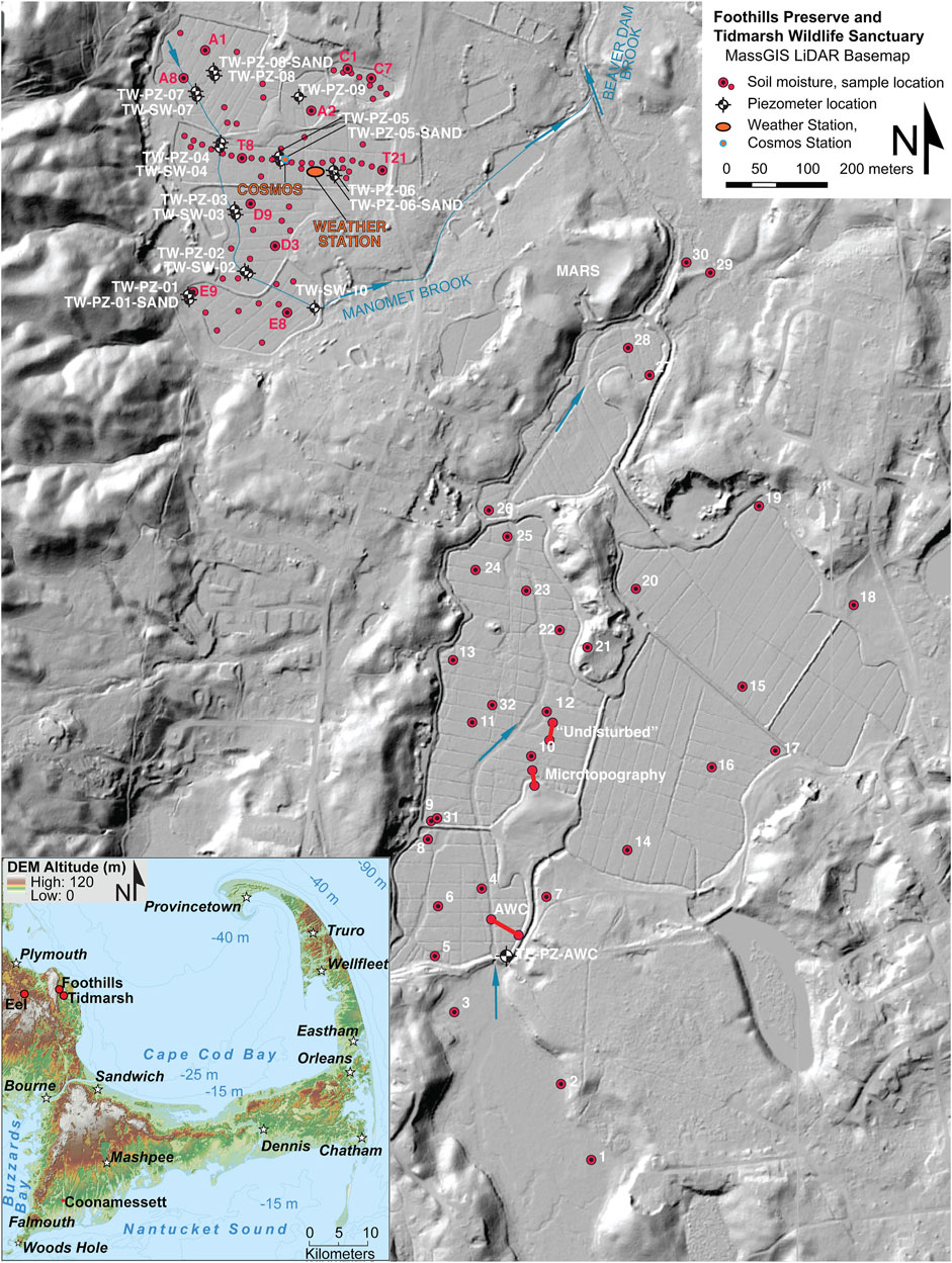
FIGURE 1. Shaded relief LiDAR terrain DEM showing the locations of samples, monitoring, and piezometers at Foothills Preserve (Town of Plymouth) and Tidmarsh Wildlife Sanctuary (Mass Audubon) on a shaded relief LiDAR (available at https://docs.digital.mass.gov/dataset/massgis-data-lidar-terrain-data). Stream flow direction arrows. (inset) Location of the two focus cranberry farms/restoration sites: Foothills Preserve and Tidmarsh on a digital elevation model (DEM) from MassGIS (Bureau of Geographic Information) Data: LiDAR Terrain Data Mapped by the Massachusetts Geological Survey (https://mgs.geo.umass.edu), Stephen B. Mabee, personal communication.
Foothills Preserve occupies a low “pit” in the landscape called a kettle hole. As the last glaciation was concluding 16,000 years ago, glaciers retreated to the north. During glacial melt and retreat, meltwater carried large quantities of sediment, and occasionally large chunks of ice downstream. These large, abandoned ice chunks sunk into and were surrounded by sediment. When they eventually melted, they left behind pits in the landscape: kettle lakes, many of which (including Foothills Preserve) eventually filled in with peat. These peatlands supported a variety of wetland plants, including the native cranberry plant (Vaccinium macrocarpon). Cranberries, as they grew naturally, were enjoyed as sasumuneash for 12,000 years by the Wampanoag people. Commercial monoculture cultivation of cranberries began in the mid-1800s, and the peatlands, wetlands, and low-elevation wet regions of southeastern Massachusetts were increasingly engineered to favor cranberry production. Over the first ∼100 years of commercial cultivation, Massachusetts lost 28% of its wetlands due to anthropogenic activity including cranberry farming (Living Observatory, 2020). Farming practices were refined, pesticides were applied to control insects and plant diseases, and business was booming. But cranberry market growth could not continue forever, and several factors contributed to the slowdown: 1) growing awareness of the consequences of chemical toxins in the environment and drinking water spurred changing farming practices, 2) legislation surrounding pesticide application and waste disposal, as well as protections for wetlands were passed, 3) new high-yield varietals of cranberries were developed, 4) the market for cranberries became saturated. Massachusetts was early to wetlands protection in 1960, partly due to a pesticide scare in 1959 (DeMoranville, 2021). Not long afterward, the insecticide dichlorodiphenyltrichloroethane (DDT) was banned, the Clean Water Act passed, and federal wetlands protections were enacted (Vileisis, 1997). Even with more land and water protections in place, the price of cranberries continued to rise, peaking at the all-time high of $66 per barrel in 1996. Cranberry farms occupied a curious middle ground where they were classified as wetlands, and protected, yet also enjoyed numerous chemical application exemptions afforded to farmlands, revokable 5 years after ceasing production (Averill et al., 2008). The new cranberry varietals thrived on drier uplands, making difficult and costly cultivation on wetlands less crucial for farmers, and over time, farmers shifted away from the native wetland varietal toward the new hybrids (Hoekstra et al., 2019). When cranberries hit the lowest price ever, of $15-$18 per barrel only a few short years later in 1999, many Massachusetts farmers could no longer afford to grow cranberries on the strangely-shaped, kettle hole wetlands. Massachusetts recognized the value of wetlands to the commonwealth, and began researching the most effective ways to return these farms to wetlands through restoration, as well as supporting landowners who wanted a “green exit” with technical expertise and grant-writing support; which was formalized in 2020 (Commonwealth of Massachusetts, 2020). This history of cranberry cultivation is written on the landscape of southeastern Massachusetts and recorded under the ground as a sedimentological record. At the surface of the cranberry farm, there are layers of material that combine organic plant material from agricultural practice, including latent chemicals stored therein, and sand applied during farming: this is the anthropogenic aquifer.
In this paper, we identify and describe a unique hydrogeological unit: the anthropogenic aquifer; and research its unique characteristics and properties. A function of coupled human activity and natural organic processes, the anthropogenic aquifer is bounded on the surface by the living cranberry plants, underlain by leaf matter and a dense, intertwined mat of vines, and at the base by the post-glacial-era peat surface (Figure 2). The function of this aquifer is strongly controlled by human engineering water movement across the site, as well as by its geologic properties. A thorough understanding of this coupled human and natural system will ultimately provide critical information to practitioners seeking to disrupt its function, and return this former peatland to a wetland state. While we highlight a specific location, land use type, and morphology herein, the conceptual implications of this study can be applied more broadly to other landscapes and farmlands where human land surface manipulations have significantly altered how water moves and interacts with the land and sub-surface.
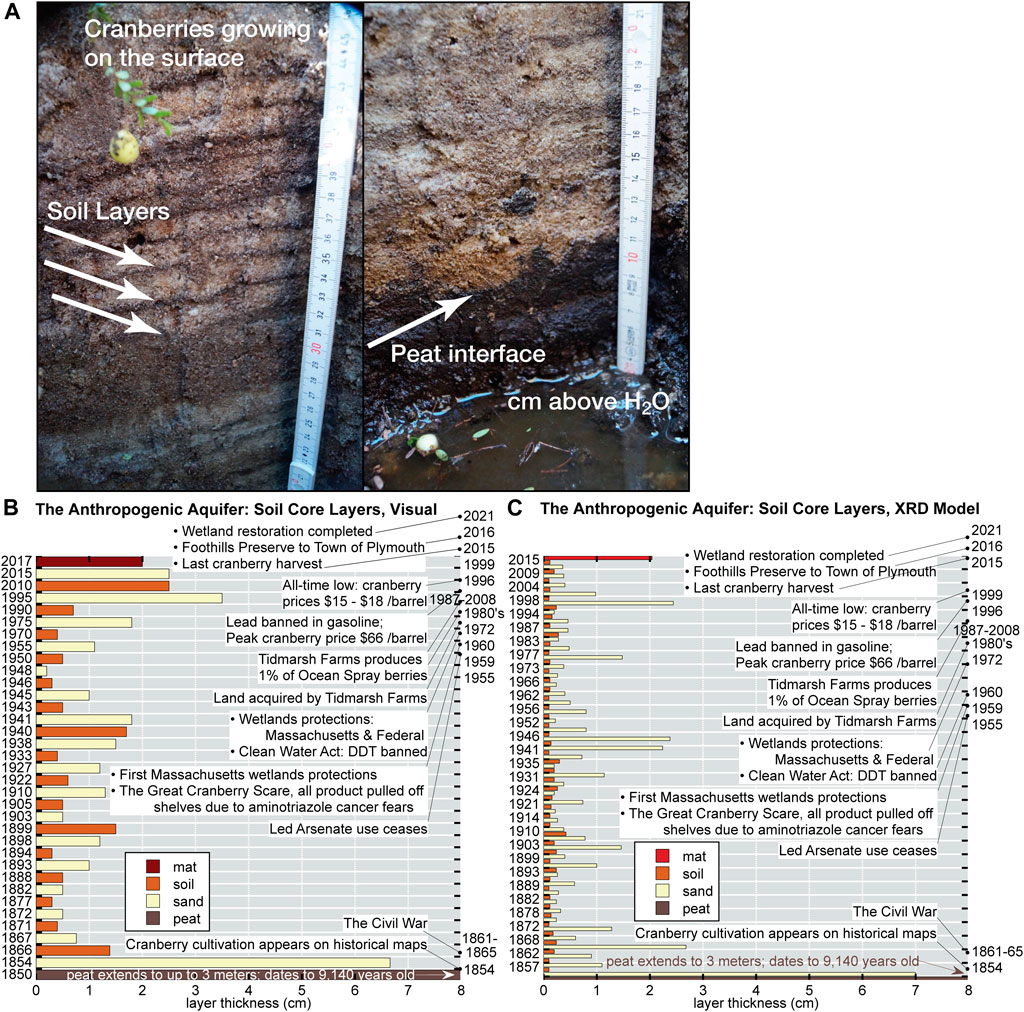
FIGURE 2. (A) The anthropogenic aquifer at Foothills Preserve is bounded by the cranberry mat at the surface and the peat at the base. (B) A visual description of a sediment core through the anthropogenic aquifer yields a kit-kat bar of alternating sand-and soil layers. (C) The XRF Os-soil proxy yielded an average sand application interval of 3.5 years, helping create the age-depth model for plotting historical events on (B) and (C).
The natural hydrology of the peatland prior to intensive cranberry cultivation would have been similar to a wet sponge, with lofty mounds of sphagnum moss pillowed just above the water surface most of the time, and a messy, multiple, or braided channel winding through and across it. The elevation of the water table within a foot of the ground surface throughout the year favors wetland plants. Sparse cranberry vines would have been an accent, climbing the sphagnum pillows and producing few fruits. Cranberries (Vaccinium macrocarpon) are wetland plants, but to cultivate them as a thick, intensely productive mat requires engineering.
The kettle basins were too wet for the cranberries on the surface, so a layer of sand was applied to flatten the ground and dry the out surface to the correct moisture. Ditches were dug to drain water down to straightened, central channels and deep perimeter ditches that acted like a moat, keeping pests out. Periodically, temperatures would drop below freezing and threaten the plants. As wetland plants, cranberries can be submerged for a few days without drowning to protect them from the cold. Tall berms around segments of the farmlands were constructed to contain the “flood” (applied water), which, in order to be effective, had to get on quickly, and get off quickly–thus ditches were dug throughout the bog and a deep central channel was constructed to convey the water away. Sand was applied every 3–5 years to hold down the vines, for pest control, and to maintain a dry surface (Averill et al., 2008). Channel straightening, berms, ditches and dams all present barriers to wetland function that are addressed during restoration. This investigation explores the cumulative impact of sanding and farming practice over 150–200 years.
We collected several 1-m long, 1–1/2-inch diameter soil cores at Foothills Preserve and conducted a geologic analysis of them. This analysis, conducted initially by Casey et al. (2019), was refined by Chase (2021), and included visual description, grain size analysis with a Horiba Camsizer P4, carbon-14 dating, and x-ray fluorescence (XRF) (Figure 2). Where data were collected as time series or large data sets, the mean, standard deviation, and range was calculated for manual measurements and logger measurements.
Soil samples measuring 100 cm3 were collected using a push corer at Tidmarsh Wildlife Sanctuary and Foothills Preserve. These cores were collected as pairs, with one sample in peat below the anthropogenic layers, and one sample spanning the layers. Some were collected horizontal to layers and others oriented vertically, to analyze hydraulic properties in both orientations. A Dynamax TH2O soil moisture probe was used to measure a 10-cm integrated moisture measurement where each core was collected and along transects at both sites (Figure 1). A couple of additional 160 cm3 cores were collected to allow a simultaneous continuous EC5 soil moisture probe and HYPROP experiment to be run.
To run the HYPROP measurement, the field-moisture sample is weighed. Then it is saturated for up to 2 weeks (for peat samples) or 2 days (for sand samples) to bring it to 100% saturation. The sample is then weighed again and the experiment begins: while the sample dries evaporatively from above, potentiometers measure matric potential at two depths within the sample. When both probes experience cavitation, the experiment is complete. The weight-potential curves are processed using the METER Group Hyprop-FIT software. Sand samples took approximately 2 weeks to run, and peat samples took as long as 2 months.
We collected water samples for isotopic analysis from a range of sources during the initial site assessment. A heated tipping bucket rain gage (Young Instruments) connected to a weather station (Campbell Scientific Inc.) was outfitted with a sample collection at the outflow to capture precipitation samples. Surface water samples were pulled directly from the stream. Suspected groundwater springs were sampled by manually determining the coldest area of the spring (during the Summer; or the warmest spot during the Winter) and collecting the sample as close to that source as possible. Water samples were collected from piezometers using a vacuum hand pump. Samples were filtered with a 0.25-
Streamflow was measured using the velocity-area method (Rantz, 1982; Sauer and Meyer, 1992) with an OTT-Hydromet acoustic velocity flowmeter mounted on a calibrated wading rod. Flow was measured upstream and downstream and differenced to determine net gain or loss. A minimum of 20 velocities were collected for each discharge measurement, and channel geometries were very good, resulting in a minimal 5% error for each total discharge measurement.
Eighteen piezometers were installed at Foothills Preserve (17) and Tidmarsh Wildlife Sanctuary (1) in 2017 (Supplementary Table S1). Piezometers are constructed from 1–1/4 inch polyvinyl chloride (PVC) pipe with a solid PVC point. Screened intervals are approximately 7-cm long, consisting of 1-cm diameter holes are drilled at the bottom of the pipe, and backed with a 18x18 gauge (1.18 mm-opening) brass mesh screen. All piezometers were installed using direct push or hammer in the very soft substrate. Water levels were measured manually, and used to calibrate pressure transducer measurements (Onset Computer Corporation U20 water level and temperature loggers, accuracy ±0.44°C and ±0.3 cm). Piezometers (4) were installed up to a meter deep in the bed of the main stream channel and paired with a stilling well to measure time series of hydraulic gradients along the stream. Piezometers installed in the peat aquifer on the bog surface were also installed to approximately 1-m depth to midpoint of screen. Finally, “sand aquifer” piezometers were installed with the screened interval at the bottom of the anthropogenic aquifer, and are each paired with a bog surface (peat) piezometer. Where data were collected as time series or large data sets, the mean, standard deviation, and range was calculated for manual measurements and logger measurements.
Our goal for understanding the hydrology of the anthropogenic aquifer is to quantify how hydrologic function was altered during the period of cranberry farming land use, such that these changes can ultimately be reversed to restore wetland hydrologic function to the site. Anthropogenic changes include physical restructuring of the land surface as well as changes to soil composition, permeability, soil chemistry, soil moisture and soil organic content. Groundwater input to the site remains unchanged over time, but how and where that groundwater interacts with surface sediment and surface waters is vastly different during the farming operation, and while the site is a wetland (e.g., Jackson, 1995; Mitsch and Gosslink, 2015). As sustainer of the future wetland and a thermal buffer for many organisms facing climate change, it is essential to reconnect the groundwater to the surface; which is only possible by first identifying locations of groundwater expression.
One of three essential components that define wetlands in most regulatory frameworks is the presence of hydric soils, soils that are formed under very wet conditions and accumulate evidence of having been submerged for more time than they have been dry. Hydric soils contain a significant percentage of organic material, hold water longer than other soils, and drain poorly. None of these conditions are present in the root zone of the anthropogenic aquifer. The top 35 cm site-wide are dominated by sand, applied during farming and accumulated over the years of this land use. This zone of applied sand (from adjacent glacial outwash sand deposits) layers intercalated with agricultural soils accumulated over intervening years between applications is termed the “anthropogenic layer”. While mimicking the horizontal layered appearance of geologic strata, the provenance of the anthropogenic layers owes exclusively to human activities and uses of the land surface. In the root zone (roughly the top 10–15 cm, contained within the anthropogenic layer), in the farmed condition, organic content of soils is between 1% and 7%, and decreases with depth until the interface with peat is reached (Table 1). At Tidmarsh, four samples taken from various depths within the anthropogenic sand averaged 1% organic material. At Foothills, samples were collected from 71 sites at four depths, all within the anthropogenic layer. Organic content remains very low within the root zone and the entire anthropogenic layer, decreasing slightly with depth. Across the site, Foothills soil organic matter averages 7 ± 4% from 0 to 5 cm depth, 3 ± 2% from 5 to 10 cm depth, 2 ± 1% from 10 to 20 cm depth, and 2 ± 2% from 20 to 30 cm depth. The organic materials in the anthropogenic aquifer are also the smallest particles, but the fraction of these particles is so small, it does not register in the grainsize analysis data. Grainsize analysis from Foothills samples exhibit d10 averages 0.14 ± 0.02mm to 0.16 ± 0.04 mm from all depths (Table 1). Since d10 (representing the smallest 10% of grains by weight) is less than the highest organic content (7% from 0 to 5 cm depth), the presence and fraction of organic matter is not represented in these results. Furthermore, these particles would be better quantified using wet-preparation methods not used in this study. Mineral grains in Foothills samples exhibit an overall decrease in grainsize with depth within the anthropogenic layer, with d50 and d90 values getting smaller with depth. Across the site, Foothills d50 averages 0.48 ± 0.12 mm from 0 to 5 cm depth, 0.47 ± 0.10 mm from 5 to 10 cm depth, 0.38 ± 0.06 mm from 10 to 20 cm depth, and 0.37 ± 0.05 mm from 20 to 30 cm depth, while Foothills d90 averages 1.57 ± 1.19 mm from 0 to 5 cm depth, 1.35 ± 0.61 mm from 5 to 10 cm depth, 1.14 ± 0.44 mm from 10 to 20 cm depth, and 1.12 ± 0.54 mm from 20 to 30 cm depth. In a natural system coarsening toward the surface can be a function of freeze-thaw processes preferentially pushing larger grains upward, but it is unclear whether enough time has elapsed in the anthropogenic aquifer for freeze-thaw processes to produce this distribution. Below 35 cm at Foothills and 45–50 cm at Tidmarsh, there is an abrupt transition to peat. This peat was accumulated following the retreat of the last glaciation 12,000 years ago. Carbon dated cores from Foothills Preserve have identified basal peat layers as old as 9,140 ±110 years, with the surface of the peat approximately 200 years old, when farming (and sanding) began. A peat sample from near the top of the accumulated peat at Foothills was 86% organic material, and the five Tidmarsh peat samples were 87 ± 7% organic material. Organic material retains more moisture for a longer period of time. At Foothills and Tidmarsh, peat was 95–100% saturated when collected. Field moisture of Tidmarsh sand samples averaged 32%, and dropped to 10% during transport to the lab, while peat samples averaged 85% and dropped to 79% over the same period. At Foothills, gravimetric soil moisture followed a similar trend: the samples with the highest organic content (at the ground surface) also have the highest soil moisture, and both organic content and soil moisture decrease with depth. The samples with the highest organic content also retain more moisture during transport. Across the site, Foothills gravimetric soil moisture averages 33 ± 28% from 0 to 5 cm depth, 28 ± 13% from 5 to 10 cm depth, 27 ± 11% from 10 to 20 cm depth, and 25 ± 15% from 20 to 30 cm depth.
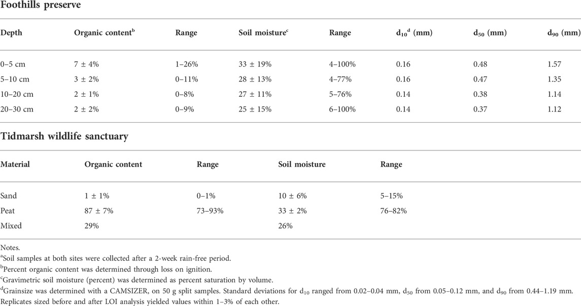
TABLE 1. Summary of pre-restoration soil organic content, soil moisture and grain size.
During her analysis of the XRF data, Chase (2021) found that there was a correlation between high Osmium (Os) detection counts and thin agricultural soil layers that accumulated between sand applications, and non-detect for Os in the sand layers. This proved a promising proxy for counting the layers, and years, since farming began. We calculated an age-depth model by assuming that each “Os-detect” layer thicker than 1 mm (scan resolution = 0.2 mm) counted as one layer, and using a starting date of 2015 (the last harvest), subtracted 3.5 years per detected layer. These parameters yielded 46 agricultural layers in the core sample and yielded a start date of 1854, the documented start of farming at Foothills Preserve (Figure 2C). Based on these ages, Chase (2021) observed lead and arsenic beginning to appear first together at 30 cm depth, when lead-arsenate was used as a pesticide. The maximum lead concentrations appear between 20 and 30 cm depth and taper off sharply when its use is curtailed by the Clean Water Act and removed from gasoline.
Peatlands may develop where relatively flat, low-lying areas with poor drainage accumulate and hold water over time. On the post-glacial pitted plain, these areas can be formed where kettle lakes pockmarked the glaciofluvial clays deposited during glacial retreat; some remained lakes and others, like Foothills Preserve eventually filled with peat. Much of the water is derived from precipitation into the surface basin. We estimate that on an average year, the 2.72 km2 (1.05 mi2) Manomet Brook surface basin would receive 130 cm (51 inches) of precipitation. Regional evapotranspiration is estimated at approximately 109 cm [43 inches, Masterson (2009)]. To a first order, we estimate the total surface runoff to be the volume that would be created by surface precipitation if applied evenly across the basin area, that this volume is approximately equal to evapotranspiration, and that the average discharge therefore represents baseflow, or the contribution from groundwater. By comparing the average baseflow (Q) to the surface area runoff (P), we estimate rainfall-runoff ratio (Q/P), or the contribution of groundwater. If Foothills discharge averages Q=56.6 L/s (2 cfs), that equates to ∼66 cm per year over the surface basin, and rainfall-runoff, Q/P indicates that 55% of discharge comes from groundwater. We measured streamflow in Manomet Brook prior to restoration at the upstream and downstream ends of the site between 2018 and 2020 (Table 2; Figure 3). Manual velocity-area discharge measurements show gains of between 19.6 and 47.1 L/s (0.69–1.66 cfs) over the 550-m reach, which is between 77% and 93% of the downstream discharge. We collected time series of stream stage upstream, TW-SW-07, and downstream, TW-SW-10. Fitting manual streamflow measurements to stage-discharge relationships, we generated a rating curve, which we applied to time series of water levels. Differencing time series of calculated stages from upstream and downstream consistently yields average groundwater contributions throughout the year of 84%.
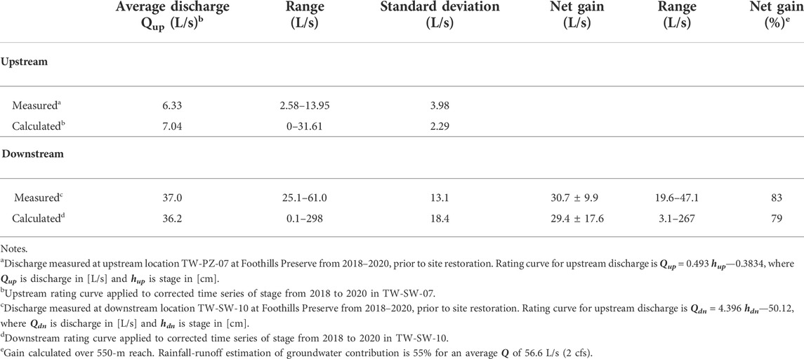
TABLE 2. Summary of pre-restoration streamflow.
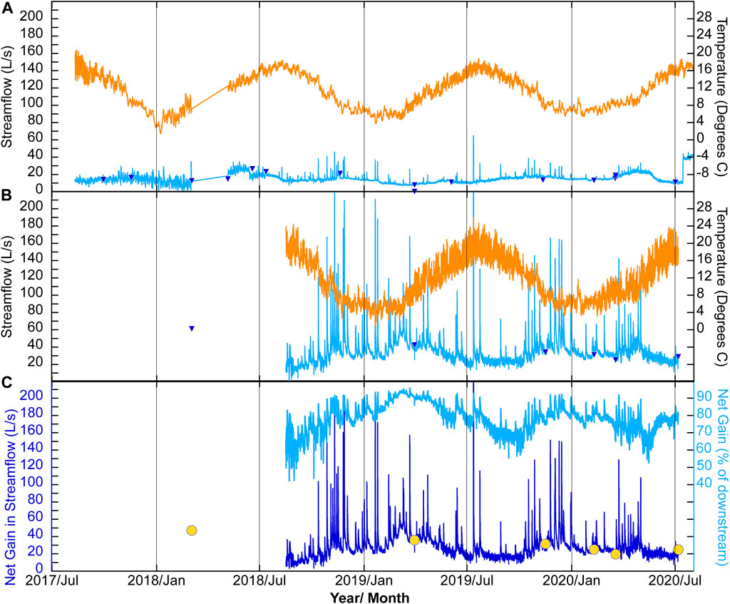
FIGURE 3. Stream flow gains at Foothills Preserve. (A) Manual measurements (symbols) and time series of discharge (Q [L/s], blue) and temperature (°C, orange) upstream, (B) downstream, and (C) net gain along the 550-m reach (∆Q [L/s], dark blue) or as a % of downstream flow (light blue).
Water levels in streambed piezometers paired with stream stage allow for calculation of hydraulic gradient. Piezometers distributed along the 550-m reach allow identification of the general location of streambed-driven groundwater gains (Figure 1B). Four streambed-stream pairs were monitored at the site, from upstream to downstream: TW-PZ-07, -04, -03, and -02; and TW-SW-07, -04, -03, and -02, and the surface-water-only at the outlet, TW-SW-10. All five surface water loggers show flashy responsiveness to storms, and very little seasonal change in water height (Figure 4; Table 3). All stream records show a large seasonal temperature signal, as well as strong diurnal temperature fluctuations. Temperatures in streambed piezometers show very little diurnal variation, span a much smaller range than the surface temperatures (Figure 5; Table 3), and show much less responsiveness to precipitation events. Large negative excursions in water level height in piezometers TW-PZ-03 and -04 occur after most of the water in the piezometer was pumped out for sampling (approximately 500 ml). Recovery times for piezometers screened in peat range from 7 to 70 days after sampling (Tables 3 and 4). Box plots of these data (Figure 6) show (B) stream depth increasing downstream, except where the stream becomes wider and shallower at the outlet TW-SW-10. The water level above the streambed in the piezometers shows (A) piezometer head increasing downstream also, but at a faster rate than the increases in stream level. This results in an increasingly positive gradient from upstream to downstream (Figures 7, 8), with a particularly large jump at TW-PZ-02. Average gradient (∆h/∆z) = 0.02 ± 0.02, 0.02 ± 0.03, 0.03 ± 0.04 and 0.14 ± 0.06 from manual measurements in TW-PZ-07, -04, -03, and -02, respectively; and Average logger-calculated ∆h/∆z = 0.03 ± 0.02, 0.01 ± 0.04, 0.04 ± 0.06, and 0.16 ± 0.01 in TW-PZ-07, -04, -03, and -02, respectively.
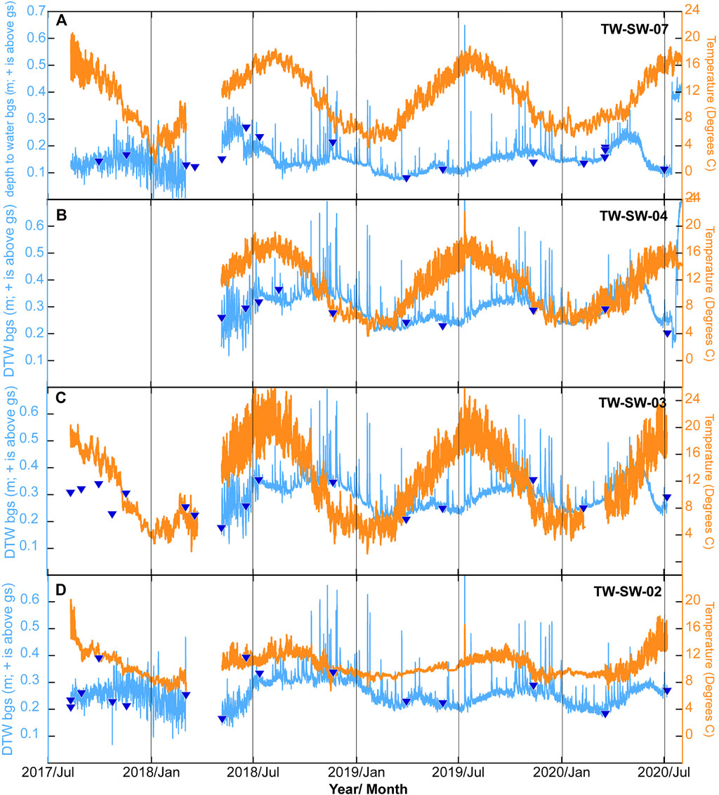
FIGURE 4. Foothills Preserve stream surface water levels (depth to water below ground surface, DTW bgs, [m] above streambed is positive, blue; symbols = measured) and temperatures (°C, orange) from upstream to downstream at Foothills Preserve: (A) TW-SW-07, (B) TW-SW-04, (C) TW-SW-03, and (D) TW-SW-02.
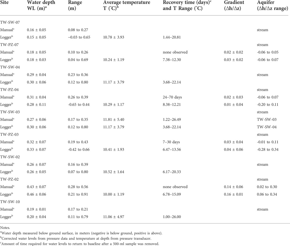
TABLE 3. Summary of pre-restoration water levels and temperatures in stream piezometers.
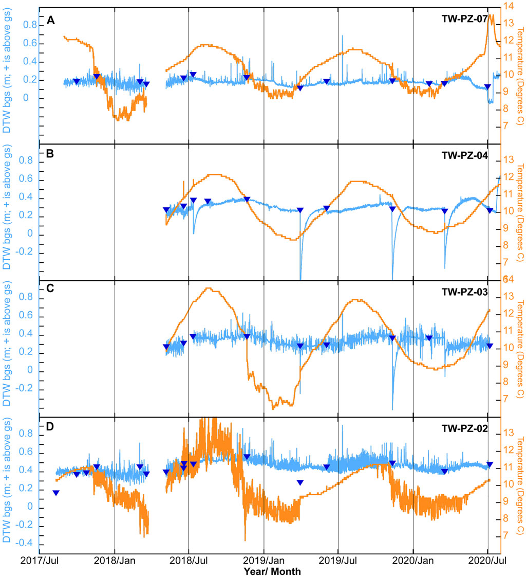
FIGURE 5. Foothills Preserve stream piezometer water levels (depth to water below ground surface, DTW bgs, [m] above streambed is positive, blue; symbols = measured) and temperatures (°C, orange) from upstream to downstream at Foothills Preserve: (A) TW-PZ-07, (B) TW-PZ-04, (C) TW-PZ-03, and (D) TW-PZ-02. Note the large negative WL excursions from water sample collection in TW-PZ-04 and -03. Recovery times are shown in Tables 3 and 4.
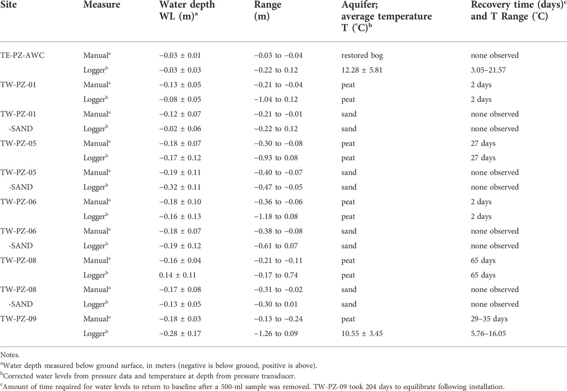
TABLE 4. Summary of pre-restoration water levels in bog piezometers.
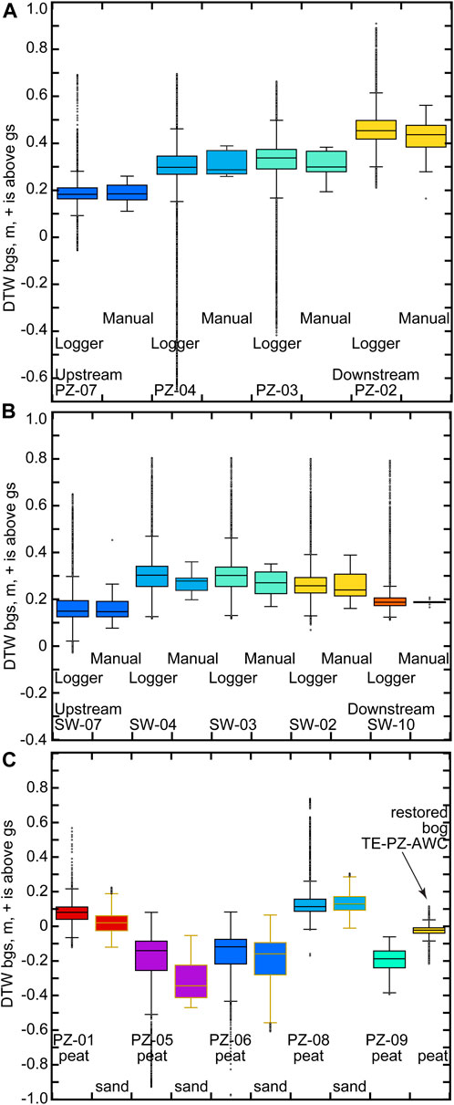
FIGURE 6. Box plots of Foothills Preserve water levels (meters below ground surface; positive is above streambed) from upstream to downstream, manual measurements and logger data; (A) in streambed piezometers: TW-PZ-07, TW-PZ-04, TW-PZ-03, TW-PZ-02, (B) from the stream surface TW-SW-07, TW-SW-04, TW-SW-03, TW-SW-02 and TW-SW-10, (C) and in bog surface peat and sand-aquifer piezometers: TW-PZ-01 and -SAND, TW-PZ-05, and -SAND, TW-PZ-06, and -SAND, TW-PZ-08 and -SAND, TW-PZ-09, and TE-PZ-AWC.
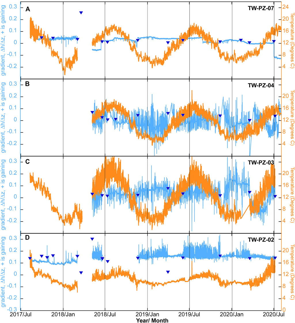
FIGURE 7. Foothills Preserve streambed hydraulic gradients, (∆h/∆z, blue; symbols = measured) and stream temperatures (°C, orange). Positive gradients indicate gaining, or upwelling conditions, and negative values are losing. From upstream to downstream: (A) TW-PZ-07, (B) TW-PZ-04, (C) TW-PZ-03, and (D) TW-PZ-02.
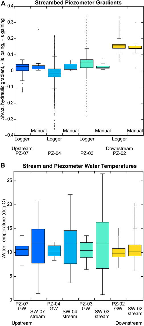
FIGURE 8. Box plots of Foothills Preserve (A) streambed hydraulic gradients, ∆h/∆z. Positive gradients indicate gaining, or upwelling conditions, and negative values are losing. From upstream to downstream piezometers: TW-PZ-07, TW-PZ-04, TW-PZ-03, and TW-PZ-02. (B) Temperatures in streambed piezometers (GW) and stream (SW) from upstream to downstream -07, -04, -03, and -02.
Depth to water below the farmed surface is compared across the site in peat piezometers in the streambed (Figure 6A; Table 3), peat piezometers, and sand piezometers on the bog surface (Figure 6C; Table 4). The deepest depths to water occur in the sand (anthropogenic) aquifer near the center of the bog. These average water levels are consistently lower than their paired peat piezometer, indicating upward pressure from groundwater into the anthropogenic aquifer. By comparison, water level at Tidmarsh piezometer TE-PZ-AWC, which was restored in 2015, hovers very near the ground surface throughout the year, has very little response to storms and very low variability. Two piezometer pairs show a strong correlation between sand and peat aquifer levels, and low variability: TW-PZ-01 and -08. In addition, the water table in the anthropogenic aquifer at TW-PZ-01-SAND is near or above the ground surface.
Understanding conditions are present in the root zone of the anthropogenic aquifer requires analyzing the material properties of the aquifer. The sand-dominated anthropogenic aquifer mimics the horizontal layered appearance of geologic strata, which rather than having been laid down by geologic phenomena, were applied regularly (on average every 3–5 years) as part of the farming practice (Averill et al., 2008; DeMoranville, 2021). Sand layers and agricultural soils accumulated in the spans between them over the 161 years since the initiation of farming on the site in 1854 and its conclusion in 2015 comprise the top 35 cm of material at Foothills, and nearly 50 cm at Tidmarsh (Kennedy et al., 2018a use GPR studies to estimate that 50 cm is average for the anthropogenic aquifer thickness across southeastern Massachusetts). In order to determine the hydraulic properties of the anthropogenic aquifer we used two approaches: parametric calculations of bulk properties based on site measurements and geometry, and laboratory tests using a HYPROP.
We collected a limited number of samples for HYPROP analysis, as these are expected to be broadly representative, given the uniformity of the substrate at our site (Payne and Theve, 2015) and across similar sites in the region (Kennedy et al., 2018). Average material properties (hydraulic conductivity, K) determined through best fit to the experimental data are summarized in Table 5. A sample collected in the anthropogenic sand in the horizontal direction produced properties that were 54 times more conductive (Kh = 20.6 cm day−1) than a sand sample oriented in the vertical direction, where water has to pass through the organic layers between sand layers (Kv = 0.381 cm day−1). In the peat, samples oriented in the horizontal direction produced properties that were an order of magnitude more conductive in the horizontal direction (Kh = 3 cm day−1) than in the vertical direction (Kv = 0.353 cm day−1). These low conductivity values are consistent with other, more extensive peat studies (e.g., Beckwith et al., 2003; Dettmann et al., 2014; Rezanezhad, 2016). Some natural permeability in peat is structural–owing to relict intact plant stems, or fractures in the peat matrix. During eventual restoration actions, some peat will be broken up and mixed in with sand layers. In an effort to experimentally capture the impact of these actions on the peat properties alone, we broke up a dried peat sample, rehydrated it, and repeated the HYPROP experiment. The data and subsequent curve fit from this test were poor, but the rough fit indicated that conductivity would be approximately an order of magnitude higher than for undisturbed peat.
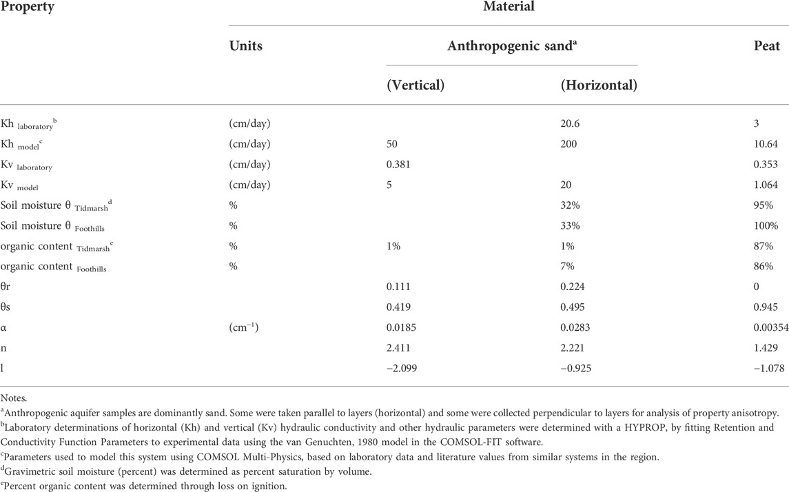
TABLE 5. Summary of material hydrogeologic properties.
For the parametric calculations of bulk properties, we examined literature values from similar systems in the region (Neill and Deegan, 2020; personal communication; Neill et al., 2017; Kennedy et al., 2018; Kennedy et al., 2020; Living Observatory, 2020) in addition to values used in regional modeling studies (e.g., Masterson et al., 1997; Masterson et al., 2009), and set up a model representing Foothills Preserve using COMSOL Multi-Physics (Ito, 2021). Model inputs were derived from the hydrologic data discussed above, and material properties had to produce outputs that could be validated by field measurements as well. It would have been numerically inefficient and computationally expensive to simulate every individual sand and organic layer within the anthropogenic aquifer. Instead, bulk properties were assigned to the entire anthropogenic aquifer, with an anisotropy value equivalent to that produced by sediment layering as described above from HYPROP measurements, and consistent with harmonic mean calculations of flow in layered systems. This approach produced material properties (hydraulic conductivity, K) that were an order of magnitude more conductive in the horizontal direction (Kh) than in the vertical direction (Kv) in the anthropogenic sand, which was 20 times more conductive than the underlying peat (Table 5). These parameters are consistent with observations from nearby Tidmarsh Wildlife Sanctuary (Hare, 2015; Hare et al., 2017; Hoekstra et al., 2019). In addition, if we use the XRF-Os-agricultural soil proxy (Figure 2C), the soil-to-sand distribution yields Kh/Kv = 15, and using Chase’s visual description (2021) (Figure 2B), the soil-to-sand distribution yields Kh/Kv = 25.
From 2017 to 2019, a large-scale campaign to classify the isotopic characterization of the waters of Massachusetts was conducted, and culminated in the classification of the means, variability, trends and local water lines for precipitation, surface waters and groundwaters (Cole and Boutt, 2021). According to the “Iso-scape” study, our research area lies within Zone III, the eastern portion of the state, characterized by glacial outwash groundwater aquifers, and copius groundwater discharge. Comparing the water isotope values from our samples to statewide data reported by Cole et al. (2021) helps confirm the source of these waters as deriving from groundwater in the region. Supplementary Figure S1 shows four trendlines: the Global Mean Water Line (GMWL), the Massachusetts MWL (MA MWL), the Massachusetts Surface Water Line (MA SWL), and the Massachusetts Groundwater Line (MA GWL). Also shown are all of the Foothills Preserve precipitation Oxygen-18 (
We identified a number of springs at Foothills Preserve while it was actively farmed for cranberries, that took the form of holes, sinks and wet areas on the ground surface. Guided by the nearby observations of Hare, (2015, and Hare et al., 2017), that identify two mechanisms for groundwater discharge into peatlands, we separated these geographically into those occurring at the margins of the bog and those occurring toward the interior. Oxygen-18 (
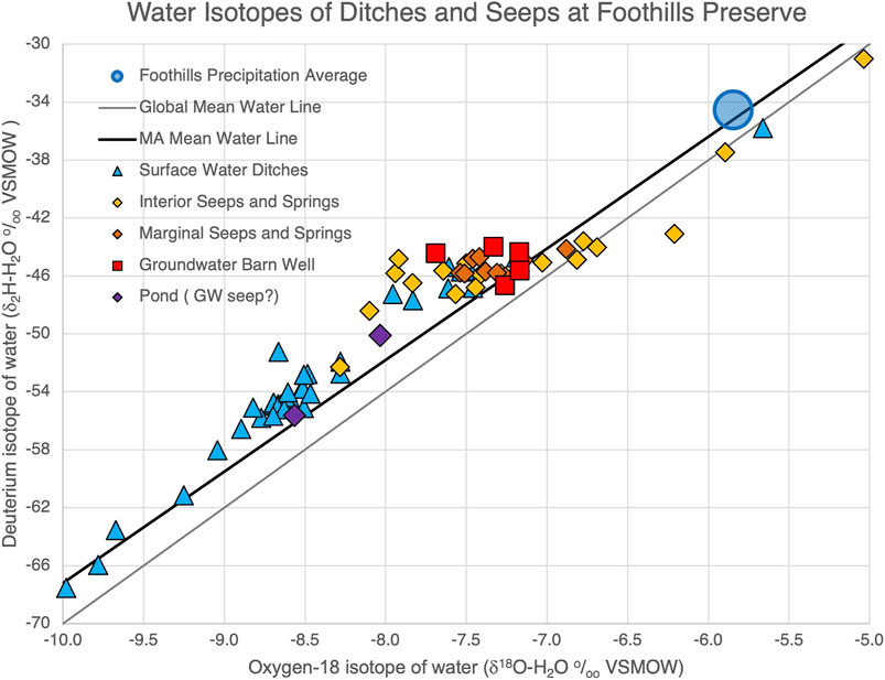
FIGURE 9. Isotopic composition of Foothills Preserve surface waters. Trendlines shown include the Global Mean Water Line (GMWL, thin grey), and Massachusetts MWL (MA MWL, thick black). Symbology of sample sources include: Average Foothills Preserve precipitation (large blue circle), surface water ditches (cyan triangle symbols), seeps and springs from the bog interior (yellow diamonds) and bog margins (orange diamonds), the Barn groundwater well (red squares), and pond (purple diamonds).
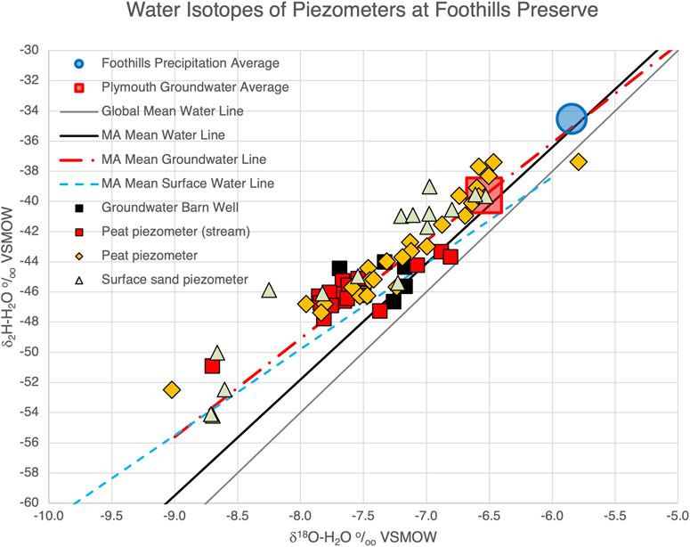
FIGURE 10. Isotopic composition of Foothills Preserve waters collected from piezometers and wells. Trendlines shown include the Global Mean Water Line (GMWL, thin grey), the Massachusetts MWL (MA MWL, thick black) the Massachusetts Surface Water Line (MA SWL, simple dash, cyan), and the Massachusetts Groundwater Line (MA GWL, dot-dash, red); and average groundwater from the Plymouth area (large red square) from Cole and Boutt (2021). Symbology of sample sources include: Average Foothills Preserve precipitation (large blue circle), peat piezometer samples installed in the streambed (red squares), peat piezometer samples installed on the bog surface (yellow diamonds), sand aquifer piezometers (green triangles), and the Barn groundwater well (black squares).
Figure 10 shows how Foothills Piezometer waters’ isotopic composition relates to local and regional water sources. The groundwater immediately underneath the site, as measured in the Barn well, is depleted slightly with respect to groundwater elsewhere in the Plymouth area. This contrasts with our local precipitation average which appears enriched. However, the Foothills precipitation data have not been volume weighted, so this average may be skewed. The piezometers screened deepest into the peat are the streambed piezometers. These stream-peat isotope values (red squares) generally cluster tightly around the GW Barn well values, confirming their groundwater provenance. The single depleted outlier was from TW-PZ-02, and is inconsistent with the remaining samples from that location. Peat piezometers from the bog surface (yellow diamonds) overlap the stream piezometer values, and also extend in the enriched direction toward the regional groundwater average and local precipitation average, along a mixing line that appears enriched with respect to the MA MWL, potentially indicative of increased humidity. A single enriched value from TW-PZ-05 is inconsistent with the remaining samples from that location, as is the single depleted outlier from TW-PZ-01. These endmembers establish the sources for possible water sources for the Anthropogenic aquifer. Are these waters primarily derived from surface water sources, flowing in laterally from upgradient? Or, do waters push up into the Anthropogenic aquifer from the peat below, generating a groundwater source signature? Evidence from Figure 10 points to both. The sand aquifer samples, typically only occupying 10–20 cm of water in the piezometer at any time, span isotopic compositions ranging across roughly the same range as the bog surface peat piezometers. One exception is TW-PZ-08-SAND, which consistently shows a distinctly surface water source isotopic composition, depleted relative to groundwater, and consistently so across time.
Finding groundwater on an active cranberry farm involves careful observation and documentation of multiple lines of evidence. Often, the most obvious evidence appears in the vegetation: the presence of duckweed in spring pools, sphagnum mosses along ditch edges, or cattails in unexpected places can all serve as indicators. Next, monitoring and mapping of temperature is a useful determinant of groundwater location: during hot Summer months, when surface waters warm and groundwater remains cooler, a thermometer can provide quick confirmation of a source. In winter, when the ground is frozen and surface waters are very cold, warm groundwater will rise, and can be imaged on the surface using thermal cameras (e.g. Deitchman and Loheide, 2009). We can then collect groundwater samples from these areas and confirm the relative intensity of groundwater inflows at these locations. In peat basins such as these, which fill glacial kettle holes, groundwater enters either at the location of maximum curvature of the basin (typically along the edges or margins), or through fractures, macropores (remnant plant stems), or other disruptions in the peat structure (e.g., Hare et al., 2017). At Foothills Preserve, linking the combined evidence provided a visual sketch as to where groundwater input was most dominant. One trace of a groundwater-dominated path was highlighted in the Living Observatory’s Learning from the Restoration of Wetlands on Cranberry Farmland: Preliminary Benefits Assessment report (2020); and maps out where a stream channel might have been prior to cranberry cultivation. Along this location, groundwater might have established pathways to the surface, that remained in spite of land surface alterations, and left evidence behind. Restoration practitioners may choose to optimize this existing pathway, and incorporate it into restoration design. The single marginal spring sample that falls outside the range of the GW well samples on Figure 9 comes from this former channel location, at the precise spot where it intersects an existing ditch, which also derives water from the interior. An extensive investigation utilizing thermal imagery collected from unmanned aerial sensors (UAS) compares the winter thermal signature of Foothills Preserve before and after restoration to identify the surface expression of groundwater springs, and quantify the change in the surface extent after restoration (Watts et al., 2022, in review).
There is a large concentration of interior seeps that plot isotopically as sourced from groundwater (Figure 10) to the south of TW-PZ-08, and downstream of TW-PZ-07. The cranberry mat is sinking into small holes on places in this area. Where waters from these groundwater inflows join the main channel, surface water springs appear in the isotopic range of groundwater, isotopically (Figure 9). As another significant source of groundwater, practitioners may target this location for groundwater capture, to feed and sustain the future wetland (Beechie et al., 2010; Price et al., 2016). Similarly, other areas that have already collapsed and significantly transformed into more wetland and less farm surface naturally, may show significant groundwater inflows. The northern-most surface water sample in Figure 9 comes from one such location, plotting isotopically most similar to average precipitation. For these, practitioners may opt to leave these sections alone, and allow them to continue the trajectory they are already on towards increased wetland function.
Streamflow data also yield key information about groundwater inflows to the wetland. Groundwater inflow throughout the year is crucial to the resilience of a functioning wetland, and the consistent ∼84% gain of downstream flow gained over the 550-m of stream is a significant amount of groundwater inflow, indicating clearly that this site possesses the hydrology to support a self-sustaining wetland system (Wohl et al., 2005). This simple metric, and knowing that it will be constant and predictable over time, is likely the single most important factor for a successful wetland restoration.
The hydraulic gradients coupled with stream and groundwater temperatures also give an indication of the location and intensity of groundwater inflows. Water levels in the stream and piezometer at TW-PZ and SW-07 are tightly coupled, yielding a very constant, near-zero hydraulic gradient with time. A significant rise in stream level, without a change in upwelling groundwater from below, may lead to a shift in gradient to negative, pushing water downward into the subsurface at this location.
The increasingly positive hydraulic gradients with increasing distance downstream are evidence of the increasing contribution of groundwater to the system with distance downstream. While the net discharge confirms these total gains along the reach, the mechanism may not be upwelling through the streambed as it is in many alluvial systems. Since the main channel has been straightened, and was constructed to efficiently drain the landscape quickly, the channel bed is deeper below the nearly flat land surface as it traverses downstream. Near TW-PZ-07, the channel bed is ∼0.5 m below the bog surface. By the time the channel reaches TW-SW-10, it is nearly ∼2 m below the bog surface. It is therefore possible that since each streambed piezometer penetrates a deeper elevation of the same peat aquifer, relative to a datum, that this drives the increase, and increasingly gaining hydraulic gradients observed in these piezometers. This observation appears to be confirmed by Figures 6B and 8A.
Stream temperatures add additional information about groundwater inflow. The range of diurnal temperature variability increases with increasing distance downstream, from TW-SW-07 to SW-04 to SW-03. This reflects the increased heating in the stream channel as the water is exposed to warm air–surface water further downstream has longer to heat up. Temperature at TW-SW-02 is completely different: the range of surface temperatures is clearly in the groundwater range, rather that the solar-heated surface range, and the times of year when diurnal variations are observed reflect different processes than solar heating. Several springs were identified in and near the channel upstream of TW-SW-02 with thermometers, thermal imagery, observations and isotopes (one, which we named “the gusher”, shows isotopic composition consistent with groundwater). Descending streambed or not, this area of the bog clearly has abundant groundwater inflows. In fact, the magnitude of the groundwater contribution here is sufficient to yield a lower average temperature at TW-SW-10 than at -03 and -04, due to the added influx of relatively colder groundwater. The combination of thermal data from this study and from Watts et al. (2022) (in review 2022) together with isotopic data provide robust quantification of a consistent, significant groundwater source that will likely sustain this wetland ecosystem even under the increasing pressures from climate change.
Depth to water below the farmed surface is a function of the upward pressure of groundwater flowing in from the peat below, and the efficiency of the lateral drainage through the overlying anthropogenic aquifer to the ditches. The Anthropogenic aquifer acts as an accelerant for lateral hydrologic flow, producing variability in the depth to water level across the farmed surface. Figure 6C illustrates both this variability, and response, in piezometers close to groundwater sources -01 and -08. TW-PZ-08 and -08-SAND are located where multiple small springs are collapsing the bog surface and allowing groundwater to flow to the surface. Here, the water level is very near the bog surface, and the level in the sand aquifer is almost identical to the peat aquifer level. TW-PZ-01 is an even more extreme example, where the sand piezometer show water levels at or even above the land surface. This piezometer is located at the very western edge of the bog, the side where the Pine Hills moraine is located, and the direction from which regional groundwater flows. A gentle gully in the hillslope upgradient seems to funnel water in the direction of TW-PZ-01, and spotted salamander eggs were observed in the perimeter ditch adjacent to it. All of this evidence points to strong groundwater inflows here, and possible upwelling pushing water upward from peat into sand. The depth to the water table below the ground surface is a key indicator of which type of plants, wetland or upland, are likely to survive and thrive, so documenting this level, and its evolution with restoration, is key to tracking the impact of restoration at sites like this one.
As part of the groundwater modeling work (Ito, 2021), we use several calculations and estimates from other studies in the region of evaporation to inform the water table height that results from the modeling work. Those estimates put the total evaporation at between half or equal to the amount of groundwater recharge entering the site from below. Such a large volume of groundwater input compared with a relatively small volume of evaporation almost always results in water ponding and export from the site. In order to maintain a high water table within the root zone throughout the growing season such that a resilient wetland ecosystem results, in addition to plugging the ditches and adding sinuosity to the stream channel, the preferential horizontal flow within the Anthropogenic aquifer must be disrupted. The parametric study conducted by Ito (2021) confirms that even a modest amount of disruption (e.g., including less than 25% peat randomly within the Anthropogenic aquifer) is sufficient to pond water and create favorable conditions for wetland development. This evidence points to favorable trajectories in multiple metrics (Alderson et al., 2019).
Peat develops in layers, much like glacial ice, where the top fluffy layer is loose snowflakes, and with each successive depositional layer, the layers below become more and more compacted until they become solid rock ice at the deepest depths. For peat, those top layers of living and recently dead plants can be extremely permeable (Holden and Burt, 2003). After 100 years or so, most peat reaches maximum compaction and very low permeability (e.g., Uhlemann et al., 2016). Fortunately for the future restoration of Foothills, this peat has been compacting for the last 161 years, and has been further compressed by farming activities and a thick, dense layer of sand and cranberry mat on top of it. HYPROP analyses revealed the peat to have very low permeability, which will be very useful for blocking flow and ponding water in the wetland. Even if the peat is broken up, it will only gain ∼1 order of magnitude more permeability, still resulting in a relatively impermeable substrate which, if mixed with sand, will help to break up the continuous, high permeability layers of the Anthropogenic aquifer.
Mixing highly compacted underlying peat with the anthropogenic aquifer materials is likely to produce several important changes that will contribute to a successful restoration. One increasingly popular technique for breaking up these layers is through the creation of microtopography, which is showing promising results (e.g., Moser et al., 2007; Rossell et al., 2009). Microtopography creates ground surface elevations that span from below the water table (generating small ponds where amphibians and other aquatic creatures can thrive), to well above it, creating a range of habitats. In addition, by mixing more organic material into surface soils, water retention in the surface soils will increase, making the root zone soils more resilient to the impacts of climate change, and more able to retain moisture through longer dry periods between storms. The bulk permeability of these mixed organic-and-mineral soils will decrease, retaining more water on the land surface. As shown by Ito (2021), even a small amount of mixing produces this outcome. Finally, the relic seedbank present within the organic layers, when brought to the surface, can help seed and replenish the site with native wetland vegetation.
In order to place the site within its broader groundwater context, it is worth considering the state of regional groundwater feeding into the wetlands: is it altered, improved or depleted? Our study region lies within a significant groundwater discharge region, and groundwater comprises a significant fraction of stream surface flows (50–100%). Initial estimates, and estimates from other studies (e.g., Masterson, 2009), attribute ∼55% of the discharge to groundwater. Accounting for evapotranspiration, our direct measurements indicate that groundwater, prior to restoration, represents an even greater fraction of discharge: 79–83%. Groundwater at this location is thus deemed to be in an “improved” state. However, to successfully restore the site to wetland function, less of the groundwater-derived surface flow must exit the site, and more must be retained in soils and as ponded water. With the exception of locations very proximal to the coast which may experience some saltwater intrusion due to groundwater pumping, groundwater in the region remains in a relatively unaltered state, with minor depletion from localized pumping of small scale supply wells (Masterson, 2009). Considering some of the detail present in streamflow data can help with additional design considerations. Streamflow changes very little upstream, which made the generation of a rating curve there difficult. At times, plants and algae had to be cleared from the channel to measure flow, and differences in stage were within measurement error. Despite the difficulty, two observations are clear: the upstream rating curve is very flat, and even if stage changes, it doesn’t affect the flow, which is essentially a measure of groundwater flowing from the concentrated spring inputs upstream (largely from one of the collapsing areas we nicknamed “the chicken foot”). In addition, stream velocity is slow, averaging 5.5 cm/s (∼0.2 ft/s). Precipitation events cause water to rise, but also to spread out and slow down (as a wetland tends to do, a very useful benefit from wetlands is flood capture): the highest discharge we measured upstream was during a Nor’easter storm, with over twice the average discharge but half the average velocity. Downstream flows behave very differently than upstream flows. The behavior of the streamflow downstream is a product of all of the groundwater gains along the reach, but also of the intense drainage system set up for farming–it was designed to shunt water off as quickly and efficiently as possible. In addition, waters entering the Anthropogenic aquifer from precipitation above or groundwater below quickly flow laterally along the layers (15–25 times more efficiently than vertical flow) and out to the drainage ditches. Together, these factors cause the hydrograph downstream to be flashy: quick to rise, quick to fall, and strongly dependent on stage height. The slope of the rating curve downstream is an order of magnitude higher than it is upstream. Flashy water height is evidenced along the length of the reach, as shown in the surface water levels from stilling wells; yet the sensitivity to this parameter downstream, which reflects the full hydrologic impact of the cranberry farm alterations, is outsized, relative to this impact upstream, which experiences far less of it. Ultimately, disrupting both the extremely effective water-drainage structures, ditches and channels, as well as the efficient preferentially lateral flow paths of the Anthropogenic aquifer will increase the residence time of water on the site, making the downstream rating curve look more like the upstream rating curve. Additional features that slow flow, such as increased sinuosity, logs, sticks and habitat features in the channel, and in-channel aquatic vegetation, will all promote slower, ponded water. Landscape-scale visualization of the locations of groundwater inputs, such as is achieved by Watts et al., (in review, 2022) can help guide restoration and locate specific intervention actions.
Based on the scenarios tested by Ito (2021), we expect that disrupting the Anthropogenic aquifer by breaking up the continuous, high permeability sand layers with chunks of relatively impermeable peat will successfully hinder the preferential flow paths that have developed in it and lead to a substrate more capable of supporting a wetland. The underlying presence of (dominantly) peat and (on the eastern margin) clay that can hold significant amounts of water will bolster the ability to hold water in the root zone on this landscape. By incorporating the organic, hydric soils into the surface layers will both expose the wetland seedbank to favorable growing conditions, but will also accelerate the return of fully functioning wetland soils (Ballantine et al., 2009). Ample evidence of stable groundwater inflows to the system provide the life force for future wetland success. Further, with increased residence time of water on the site, and increases in ponded water on the site, we expect that this site can contribute additional groundwater recharge after restoration. It is worth noting that increasing the quantity of ponded water on the surface is also likely to increase the water available for evaporation. Previous analyses of New England wetland systems concluded that recharge to aquifers in the region was about 68 cm/yr (27 in/yr), and recharge under ponds totaled 51 cm/yr (20 in/yr) when accounting for the additional water lost to evaporation. Wetlands were estimated to recharge 20 cm/yr (8 in/yr). Operating cranberry bogs were given an additional 5 cm/yr (2 in/yr) recharge due to the harvest floods forcing water into the subsurface (Zarriello and Bent, 2004; Masterson, 2009). In terms of net water export from the site, we expect that initially we may see a very marked decrease in water export from the site as water ponds and a new equilibrium is reached, corresponding to initial potential increases in recharge. As more organic material settles into the interstitial spaces of the newly mixed soils, these changes may become more modest. It is expected that ultimately the increased water holding capacity of a landscape free of ditches and drains, and soils with heightened organic content will offset some of the additional evaporation losses.
As the commonwealth of Massachusetts has recognized, restoring a freshwater wetland from a cranberry farm in a region with a great deal of groundwater discharge, sitting on top of fully developed hydric soils and a wetland seedbank has an extremely high potential for quick success. Making a new wetland where one never existed might take hundreds of years, but recovering a buried wetland from beneath a cranberry farm can be easy–with informed observations behind restoration design. Early site assessment can map the potential for groundwater input, and identify hot spots that can be targeted in designed features (See Supplementary Table S2). A full characterization of the hydrogeologic system in situ can help inform specific changes required to undo the legacy of surface land use and engineering that would otherwise leave the land surface higher above the water table than needed for a wetland to thrive, and dried out, rather than saturated. We present here observational, hydrological, thermal, and isotopic evidence of ample groundwater inflows across a broad section of the Foothills Preserve. To recover this groundwater, we delve into the human history of the surface of this landscape to understand how the anthropogenic aquifer got here, how it functions, and how, ultimately, to mix and disperse it into a restored wetland. These findings are applicable in southeastern Massachusetts, but can be applied broadly to any glaciated landscapes across North America and globally with a similar geomorphology and latitude which have cranberry cultivation on kettle peatland wetlands, that could easily be restored to wetlands. Specifically, sites that possess the hydrologic, geologic and ecologic features can be more easily reconnected to groundwater sources to restore self-sustaining wetlands.
The original contributions presented in the study are included in the article/Supplementary Material, further inquiries can be directed to the corresponding author.
CH conceived and designed the analysis, and wrote the paper, CH and EI collected the data, contributed analysis tools, and performed analyses.
This work is/was supported in part by the USDA National Institute of Food and Agriculture, McIntire-Stennis projects 1009642 and 1021302 and by Mass DER ISA # FWEHYDMONEVUMA21A, CTEMPs and the Living Observatory.
We appreciate assistance with field work provided by C. Lyn Watts, Luke McInnis, Marie Maxwell, Naomi Valentine, Cameron Richards, and many others. We are grateful to the Isoscape Project (funded by Massachusetts Environmental Trust and Massachusetts Water Resources Research Center) for assisting with water isotopic analysis. Thank you to Paul Wetzel, the Center for Transformative Environmental Monitoring Programs (CTEMPs) and Michael Cosh (USDA-ARS) for providing equipment and logistical support, Alex Hackman at Mass DER for inspiration and encouragement, as well as collaborators Living Observatory, Glorianna Davenport, Evan Schulman, Mass Audubon, David Gould and the Town of Plymouth for facilitating site access. Thanks to the thoughtful comments of three reviewers that have improved this manuscript. Finally the authors are deeply indebted to the Sheila Seaman Women Geoscientist’s Writing Retreat for a room of one’s own, time, company and support for this work.
Author EI was a graduate student at UMass for most of the research and subsequently employed by the company KoBold Metals during article writing.
The remaining author declares that the research was conducted in the absence of any commercial or financial relationships that could be construed as a potential conflict of interest.
All claims expressed in this article are solely those of the authors and do not necessarily represent those of their affiliated organizations, or those of the publisher, the editors and the reviewers. Any product that may be evaluated in this article, or claim that may be made by its manufacturer, is not guaranteed or endorsed by the publisher.
The Supplementary Material for this article can be found online at: https://www.frontiersin.org/articles/10.3389/feart.2022.945065/full#supplementary-material
Supplementary Figure 1 | Isotopic composition of Foothills Preserve precipitation water relative to Massachusetts statewide values reported in Cole and Boutt (2021). Four trendlines describe the Global Mean Water Line (GMWL, black), the Massachusetts MWL (MA MWL, grey), the Massachusetts Surface Water Line (MA SWL, simple dash, cyan), and the Massachusetts Groundwater Line (MA GWL, dot-dash, red). Also shown are all of the Foothills Preserve precipitation (blue symbols), and mean values for MA precipitation (grey circle), Foothills precipitation (blue circle), MA groundwater (red square) and MA surface water (cyan triangle).
Alderson, D. M., Evans, M. G., Shuttleworth, E. L., Michael, P., Spencer, T., Walker, J., et al. (2019). Trajectories of ecosystem change in restored blanket peatlands. Sci. Total Environ. 665, 785–796. doi:10.1016/j.scitotenv.2019.02.095
Averill, A., Caruso, F. L., DeMoranville, C. J., Jeranyama, P., LaFleur, J., McKenzie, K., et al. (2008). Cranberry production guide. Paper 8. Available at: http://scholarworks.umass.edu/cranberry_prod_guide/8.
Ballantine, K., and Schneider, R. (2009). Fifty-five years of soil development in restored freshwater depressional wetlands. Ecol. Appl. 19 (6), 1467–1480. doi:10.1890/07-0588.1
Baron, J. S., LeRoy Poff, N., Angermeier, P. L., Dahm, C. N., Gleick, P. H., Hairston, N. G., et al. (2002). Meeting ecological and societal needs for freshwater. Ecol. Appl. 12 (5), 1247–1260. doi:10.1890/1051-0761(2002)012[1247:measnf]2.0.co;2
Beckwith, C., Baird, A., and Heathwaite, A. (2003). Anisotropy and depth‐related heterogeneity of hydraulic conductivity in a bog peat. I: Laboratory measurements. Hydrol. Process. 17 (1), 89–101. doi:10.1002/hyp.1116
Beechie, T. J., Sear, D. A., Olden, J. D., Pess, G. R., Buffington, J. M., Moir, H., et al. (2010). Process-based principles for restoring river ecosystems. BioScience 60 (3), 209–222. doi:10.1525/bio.2010.60.3.7
Brown, S. C., and Veneman, P. L. M. (2001). Effectiveness of compensatory wetland mitigation in Massachusetts, USA. Wetlands 21, 508. doi:10.1672/0277-5212(2001)021[0508:EOCWMI]2.0.CO;2
Casey, J., Hatch, C. E., and Yellen, B. (2019). “Human and postglacial soil history of a wetland,” in UMass Extension CAFÉ Summer Scholars Conference Poster Presentation, Amherst, MA, 11 September 2019.
Chase, A. M. (2021). A wetland restoration at time zero: Observations from the field. May 17, 2021. UMass amherst commonwealth honors college theses and projects. Available at: https://scholarworks.umass.edu/chc_theses/.
Cole, A., and Boutt, D. F. (2021). Spatially-resolved integrated precipitation-surface-groundwater water isotope mapping from crowd sourcing: Toward understanding water cycling across a post-glacial landscape. Front. Water 3, 32. doi:10.3389/frwa.2021.645634
Commonwealth of Massachusetts (2020). Cranberry bog program. Boston, MA: Division of Ecological Restoration. Available at: https://www.mass.gov/cranberry-bog-program.
Cook, T. L., Noah, P. S., Oswald, W. W., and Paradis, K. (2020). Timber harvest and flood impacts on sediment yield in a postglacial, mixed-forest watershed, Maine, USA. Anthropocene 29, 100232. doi:10.1016/j.ancene.2019.100232
Cook, T. L., Yellen, B. C., Woodruff, J. D., and Miller, D. (2015). Contrasting human versus climatic impacts on erosion. Geophys. Res. Lett. 42 (16), 6680–6687. doi:10.1002/2015GL064436
Deitchman, R. S., and Loheide, S. P. (2009). Ground based thermal imaging of groundwater flow processes at the seepage face. Geophys. Res. Lett. 36, L14401. doi:10.1029/2009GL038103
DeMoranville, C. (2021). Interview with the 40-year veteran director of the UMass Cranberry Station discussing the evolution of cranberry production in Massachusetts. personal communication. March 31, 2021.
Dettmann, U., Bechtold, M., Frahm, E., and Tiemeyer, B. (2014). On the applicability of unimodal and bimodal van Genuchten–Mualembased models to peat and other organic soils under evaporation conditions. J. Hydrology 515, 103–115. doi:10.1016/j.jhydrol.2014.04.047
Erwin, K. L. (2009). Wetlands and global climate change: The role of wetland restoration in a changing world. Wetl. Ecol. Manag. 17, 71–84. doi:10.1007/s11273-008-9119-1
Hare, D. K. (2015). Hydrogeological control on spatial patterns of groundwater seepage in peatlands. Masters Theses 152. doi:10.7275/6446088
Hare, D. K., Boutt, D. F., William, P. C., Hatch, C. E., Davenport, G., Hackman, A., et al. (2017). Hydrogeological controls on spatial patterns of groundwater discharge in peatlands. Hydrol. Earth Syst. Sci. 21 (12), 6031–6048. doi:10.5194/hess-21-6031-2017
Hoekstra, B. R., Neill, C., and Kennedy, C. (2019). Trends in the Massachusetts cranberry industry create opportunities for the restoration of cultivated riparian wetlands. Restor. Ecol. 28, 185–195. doi:10.1111/rec.13037
Holden, J., and Burt, T. (2003). Hydrological studies on blanket peat: The significance of the acrotelm-catotelm model. J. Ecol. 91, 86–102. doi:10.1046/j.1365-2745.2003.00748.x
Ito, E. T. (2021). Testing the impact of a freshwater wetland restoration on water table elevation and soil moisture using a parametric groundwater modeling approach. UMass Amherst Masters Theses 1103. doi:10.7275/24611012.0
Jackson, S. (1995). Delineating bordering vegetated wetlands under the wetlands protection act: A handbook. Springfield, MA: Massachusetts Department of Environmental Protection Division of Wetlands and Waterways.
Johnson, K. M., Snyder, N. P., Castle, S., Hopkins, A. J., Mason, W., Merritts, D. J., et al. (2019). Legacy sediment storage in New England river valleys: Anthropogenic processes in a postglacial landscape. Geomorphology 327, 417–437. doi:10.1016/j.geomorph.2018.11.017
Kennedy, C. D., Wilderotter, S., Payne, M., Anthony, R., Buda, P., Kleinman, J. A., et al. (2018a). A geospatial model to quantify mean thickness of peat in cranberry bogs. Geoderma 319, 122–131. doi:10.1016/j.geoderma.2017.12.032
Kennedy, C. D., Alverson, N., Jeranyana, P., and DeMoranville, C. (2018b). Seasonal dynamics of water and nutrient fluxes in an agricultural peatland. Hydrol. Process. 32, 698–712. doi:10.1002/hyp.11436
Kennedy, C. D., Buda, A. R., and Bryant, R. B. (2020). Amounts, forms and management of nitrogen and phosphorus export from agricultural peatlands. Hydrol. Process. 34, 1768–1781. doi:10.1002/hyp.13671
Lewis, S., and Maslin, M. (2015). Defining the Anthropocene. Nature 519, 171–180. https://doi.org/10.1038/nature14258.
Living Observatory Ballantine, K., Davenport, G., Deegan, L., Gladfelter, E., Hatch, C. E., Kennedy, C., et al. (2020). Learning from the restoration of wetlands on cranberry farmland: Preliminary benefits assessment. Plymouth, MA: Living Observatory, 1–100. Plymouth, MA, USA. Available at: https://www.livingobservatory.org/learning-report.
Masterson, J. P., Carlson, C. S., and Walter, D. A. (2009). Hydrogeology and simulation of groundwater flow in the Plymouth-Carver Kingston-Duxbury aquifer system, southeastern Massachusetts. Scientific Investigations Report 2009–5063.
Masterson, J. P., Walter, D. A., and Savoie, J. (1997). Use of particle tracking to improve numerical model calibration and to analyze ground-water flow and contaminant migration, Massachusetts Military Reservation, western Cape Cod, Massachusetts. United States Geological Survey Water-Supply Paper 2482.
Matthews, J. W., and Endress, A. G. (2008). Performance criteria, compliance success, and vegetation development in compensatory mitigation wetlands. Environ. Manag. 41 (1), 130–141. doi:10.1007/s00267-007-9002-5
McKown, J. G., Moore, G. E., Andrew, R. P., White, N. A., and Gibson, J. L. (2021). Successional dynamics of a 35 year old freshwater mitigation wetland in southeastern New Hampshire. Plos One 16, e0251748. doi:10.1371/journal.pone.0251748
Mitsch, W. J., and Wilson, R. F. (1996). Improving the success of wetland creation and restoration with know-how, time, and self-design. Ecol. Appl. 6 (1), 77–83. doi:10.2307/2269554
Mitsch, W. J., Zhang, L., Kay, C. S., Amanda, M. N., Christopher, J. A., Blanca, B., et al. (2012). Creating wetlands: Primary succession, water quality changes, and self-design over 15 years. BioScience 62 (3), 237–250. doi:10.1525/bio.2012.62.3.5
Mitsch, W. J., and Gosselink, J. G. (2015). Wetlands. Fifth Edition. Hoboken, NJ, USA: John Wiley & Sons.
Moser, K., Ahn, C., and Noe, G. (2007). Characterization of microtopography and its influence on vegetation patterns in created wetlands. Wetlands 27, 1081–1097. doi:10.1672/0277-5212(2007)27[1081:COMAII]2.0.CO;2
Neill, C., and Deegan, L. (2020). Researchers from Woodwell Climate Research Center shared unpublished water balance and groundwater data from multiple cranberry bogs in the region as background research for the Living Observatory. personal communication. Report.
Neill, C., Scott, L., Kennedy, C., DeMoranville, C., and Jakuba, R. (2017) Nitrogen balances in Southeastern Massachusetts cranberry bogs. Report to the Buzzards Bay National Estuary Project.
Newnham, R. M., Delange, P. J., and Lowe, D. J. (1995). Holocene vegetation, climate and history of a raised bog complex, Northern New-Zealand based on palynology, plant macrofossils and tephrochronology. Holocene 5 (3), 267–282. doi:10.1177/095968369500500302
Payne, M., and Theve, M. (2015). GPR Survey of Tidmarsh west cranberry bog on beaver dam road in Plymouth. MA: USDA NRCS Investigation. April 8, 2015.
Price, J., Evans, C., Evans, M., Allott, T., and Shuttleworth, E. (2016). “Peatland restoration and hydrology,” in Peatland restoration and ecosystem services: Science, policy and practice. Editors A. Bonn, T. Allott, M. Evans, H. Joosten, and R. Stoneman (Cambridge, UK: Cambridge University Press), 77.
Rantz, S. E. (1982). “Measurement and computation of streamflow,” in USGS water supply paper 2175 vol 1 p. 1-284, Vol. 2, 285–631. doi:10.3133/wsp2175
Rezanezhad, F., Price, J. S., Quinton, W. L., Lennartz, B., Milojevic, T., and Van Cappellen, P. (2016). Structure of peat soils and implications for water storage, flow and solute transport: A review update for geochemists. Chem. Geol. 429, 75–84. doi:10.1016/j.chemgeo.2016.03.010
Rossell, I. M., Moorhead, K. K., Alvarado, H., and Warren, R. J. (2009). Succession of a southern appalachian mountain wetland six years following hydrologic and microtopographic restoration. Restor. Ecol. 17 (2), 205–214. doi:10.1111/j.1526-100X.2008.00372.x
Sauer, V. B., and Meyer, R. W. (1992). Determination of error in individual discharge measurements. USGS Open-File Report 92-144. doi:10.3133/ofr92144
Uhlemann, S. S., Sorensen, J. P. R., House, A. R., Wilkinson, P. B., Roberts, C., Gooddy, D. C., et al. (2016). Integrated time-lapse geoelectrical imaging of wetland hydrological processes. Water Resour. Res. 52 (3), 1607–1625. doi:10.1002/2015WR017932
Van den Bosch, K., and Matthews, J. W. (2017). An assessment of long-term compliance with performance standards in compensatory mitigation wetlands. Environ. Manag. 59 (4), 546–556. doi:10.1007/s00267-016-0804-1
Vileisis, A. (1997). Discovering the unknown landscape: A history of America's wetlands. Washington, D.C. Island Press, 433. ISBN: 155963314X 9781559633147.
Walter, R. C., and Merritts, D. J. (2008). Natural streams and the legacy of water-powered mills. Science 319 (5861), 299–304. doi:10.1126/science.1151716
Waters, C. N., Zalasiewicz, J., Summerhayes, C., Barnosky, A. D., Poirier, C., Gałuszka, A., et al. (2016). The Anthropocene is functionally and stratigraphically distinct from the Holocene. Science 351, aad2622. doi:10.1126/science.aad2622
Watts, C. L., Hatch, C. E., and Ryan, W. (2022). Mapping groundwater discharge seeps with thermal UAS at a wetland restoration site. Front. Environ. Sci. Environ. Inf. Remote Sens. 2022, 946565. in review.
Wohl, E., Angermeier, P. L., Bledsoe, B., Kondolf, G. M., MacDonnell, L., Merritt, D. M., et al. (2005). River restoration. Water Resour. Res. 41, W10301. doi:10.1029/2005WR003985
Woodruff, J. D., Anna, P. M., Elzidani, E. Z. H., Naughton, T. J., MacDonald, D. G., Naughton, T. J., et al. (2013). Off-river waterbodies on tidal rivers: Human impact on rates of infilling and the accumulation of pollutants. Geomorphology 184, 38–50. doi:10.1016/j.geomorph.2012.11.012
Zalasiewicz, J., Crutzen, P. J., and Steffen, W. (2012). “Chapter 32 - the Anthropocene,” in The geologic time scale. Editors M. G. Felix, G. O. James, D. S. Mark, and M. O. Gabi (Amsterdam, Netherlands: Elsevier), 1033–1040. ISBN 9780444594259. doi:10.1016/B978-0-444-59425-9.00032-9
Keywords: groundwater, groundwater-surface water interactions, ecosystem, wetland, aquifer, restoration, hydrology, resilience (environmental)
Citation: Hatch CE and Ito ET (2022) Recovering groundwater for wetlands from an anthropogenic aquifer. Front. Earth Sci. 10:945065. doi: 10.3389/feart.2022.945065
Received: 16 May 2022; Accepted: 26 July 2022;
Published: 05 October 2022.
Edited by:
Irfan Rashid, University of Kashmir, IndiaReviewed by:
Shabir Ahmad Khanday, University of Kashmir, IndiaCopyright © 2022 Hatch and Ito. This is an open-access article distributed under the terms of the Creative Commons Attribution License (CC BY). The use, distribution or reproduction in other forums is permitted, provided the original author(s) and the copyright owner(s) are credited and that the original publication in this journal is cited, in accordance with accepted academic practice. No use, distribution or reproduction is permitted which does not comply with these terms.
*Correspondence: Christine E. Hatch, Y2hhdGNoQGdlby51bWFzcy5lZHU=
Disclaimer: All claims expressed in this article are solely those of the authors and do not necessarily represent those of their affiliated organizations, or those of the publisher, the editors and the reviewers. Any product that may be evaluated in this article or claim that may be made by its manufacturer is not guaranteed or endorsed by the publisher.
Research integrity at Frontiers
Learn more about the work of our research integrity team to safeguard the quality of each article we publish.