3D hydrogeophysical characterization of managed aquifer recharge basins

Aquifers are increasingly stressed. Managed aquifer recharge provides a potential solution to mitigate this stress and provide sustainable groundwater resources. Subsurface properties are known to have a strong control on the infiltration rates that can be achieved. However, these properties are often highly heterogeneous and difficult to assess with conventional probing techniques. Here, we show the application of 3D geophysical imaging to assess the recharge potential and its variation across several basins used for managed aquifer recharge. We link in-situ measurements of saturated hydraulic conductivity with the electrical resistivity of the subsurface to establish petrophysical relationships and use those relationships to estimate the distribution of hydraulic conductivity throughout the five recharge basins. Our results show a considerable variability in the hydraulic properties, i.e., soil texture and saturated hydraulic conductivity, that have a direct impact on potential infiltration rates. We use the 3D hydraulic property distributions to model groundwater recharge and provide estimates for infiltration rates and volumes, and use this approach to assess the impact of management activities on groundwater recharge performance. Having such data not only enables us to predict infiltration rates, but also provides means for optimizing such water infrastructure.

1 Introduction

In many parts of the world aquifers are stressed, resulting in falling groundwater levels and diminishing groundwater quality due to a rapid increase in groundwater extraction and changes in precipitation pattern, which is leading to unsustainable conditions (Scanlon et al., 2012; Rodell et al., 2018). Groundwater recharge is the most important parameter to assess groundwater sustainability, particularly in arid and semi-arid regions like California, yet it is almost impossible to measure directly (Kinzelbach et al., 2003). Many indirect measurements of groundwater recharge exist, such as tracer techniques, estimations from groundwater fluctuations, or numerical models, but these are often difficult to calibrate or require considerable field effort (Singh et al., 2019). Hence, there is a need to further develop approaches that can assess potential infiltration and recharge rates through integrated approaches that include data-informed modelling.

Due to the shortage of this valuable resource, water users are facing increasing constraints in the amount of groundwater they can withdraw. With climate change exacerbating the duration of droughts, and shifting intensity and duration of precipitation events during wet periods (Füssel et al., 2012; Arias et al., 2021), water managers are seeking ways of capturing a greater fraction of precipitation to increase aquifer recharge. In California, recent regulations require that all Groundwater Sustainability Agencies become compliant with their newly formulated groundwater sustainability plans (SWRCB, 2014). One of the methods to achieve this sustainability is managed aquifer recharge (MAR). In California, local water districts and other entities are working together to identify methods to capture elevated flood flows before they reach the Pacific Ocean and to use the captured water for aquifer recharge. Ventura County Waterworks District No. 1 (VCWWD) intend to utilize the existing percolation ponds at the Moorpark Water Reclamation Facility to capture some of the yearly flood flows of the Arroyo Las Posas for managed aquifer recharge. VCWWD estimates the project could potentially recharge up to 3.7 Mm³ of captured runoff per year. However, the realization of that potential depends on how much water can be infiltrated quickly during large storm events, making the performance of infiltration ponds a key factor in overall benefit.

Hence, this study aims at developing a stream-lined workflow that provides water managers with an estimate of spatially resolved infiltration rates. We combine geophysical measurements, i.e., electrical resistivity tomography and electromagnetic induction, which are both measuring the electrical properties of the subsurface, with measurements of the saturated hydraulic conductivity of the materials forming the recharge ponds. At the site, where the groundwater level is known to be at $>$15 m depth, the electrical properties of the shallow subsurface are mostly sensitive to variations in grain size, with sandy, coarse grained layers being associated with higher electrical resistivity than fine-grained, silty or clayey materials (Banton et al., 1997; Nouveau et al., 2016). Yet, these variations in grain-size are known to have a major control on the hydraulic conductivity, and hence infiltration and recharge rates (Sterrett, 1985; Rosas et al., 2014).

These relationships between geophysical and hydrological properties have been exploited in many applications (Binley et al., 2015), and have also been used to map hydraulic properties for groundwater recharge problems. Mawer et al. (2016) used fiber optics based distributed temperature sensing to estimate infiltration rates and relate those values with electrical resistivities of the shallow subsurface. They showed that increasing resistivity (or decreasing electrical conductivity) relates to increasing infiltration rates. While this is developed on a single infiltration pond, Knight et al. (2018) made use of similar relationships to map aquifer systems for optimal recharge conditions using Airborne Electromagnetic measurements. This approach has recently been extended by Kang et al. (2021) to ease interpretation of such data over large domains. However, these small and large scale investigations are often disconnected, which is mainly due to missing instrumentation that can acquire data rapidly over different scales. Novel electromagnetic systems have been developed to more efficiently gather data at high resolution across relatively large recharge facilities (i.e., hectares to km², Behroozmand et al., 2019) and the data of those is starting to close this gap. Using these novel, towed time-domain electromagnetic (TEM) methods data can be acquired quickly at high spatial resolution (i.e., meter), yet the vertical resolution is often limited to the upper 1 or 2 m, which may not be sufficient to fully describe recharge pathways. Hence, often frequency-domain electromagnetic (FDEM) instruments are used that can sense the shallow subsurface, and can also be used to acquire data comparably quickly (Sendrós et al., 2020). Latest FDEM instrumentation make use of multiple frequencies or coil spacing, sensing different parts of the subsurface, allowing for detailed subsurface imaging, without the need for galvanic coupling to the ground.

Mawer et al. (2016) and Sendrós et al. (2020) have shown that electrical and electromagnetic geophysical methods can be used to assess spatially varying infiltration rates of recharge facilities. Here, we want to go a step forward and provide volumetric estimates of hydraulic conductivities that can be used to parameterize hydraulic models to assess the recharge performance of infiltration ponds, that in turn can be used to optimize their management. We show that using this approach, management activities can be designed that can increase the recharge efficacy considerably. Here, we show that a single survey can be used to characterize a recharge facility, but the same approach could also be used repeatably to control and enhance the performance of recharge facilities. While developed on a single site, the workflow can be considered transferable, and should be applicable to many different sites.

2 Methods

2.1 Study site

The study site is located at the Ventura County Waterworks Moorpark Reclamation Facility in Moorpark, CA. It is located along the Arroyo Las Posas River in the Little Simi Valley. The facility contains about 32 percolation ponds of which six ponds (ponds 8 to 13, Figure 1) were selected to be evaluated in this study. The site is located within the South Las Posas Basin, which has a surface area of about 41 km², and belongs to the Calleguas creek watershed. Geologically, the site is located at the western margin of the Transverse Ranges of Southern California, which is characterized by east-west oriented mountain ranges that are separated by valleys, faults, and basins. The valley fills consist of unconsolidated and semi-consolidated sediments of considerable thickness ($>$ 400 m) that range in age from the Pliocene to Holocene (FCGMA, 2016). The hydrogeology at the site is characterized by two aquifers, the upper aquifer unit, comprising alluvium and the Oxnard and Mugu aquifers, within which water is usually unconfined and found 7.5–15 m below ground, and the lower aquifer unit, comprising the Upper and Lower Hueneme, and the Fox canyon aquifer, which is confined and groundwater is usually found between 100 and 150 m depth (VCWPD, 2015). The upper aquifer comprises alluvium, and consists of lagoonal, beach, river and flood plain, artificial, and alluvial fan deposits, with coarse gravels and sands forming the Oxnard and Mugu aquifers that are a major groundwater source (Hanson et al., 2003). The lower aquifer unit comprises the Saugus, San Pedro, and Santa Barabara Formation. The Saugus Formation is comprised of terrestrial fluvial sediments, while the San Pedro Formation comprises marine clays and sands, as well as terrestrial fluvial deposits. The Santa Barbara Formation is formed of Marine shallow sands. The Santa Barbara Formation is known to be of low permeability, and hence not considered an important source of groundwater, while the overlying coarser sands and gravels of the San Pedro Formation are usually laterally extensive and more permeable, and hence a major source for groundwater (Hanson et al., 2003).

FIGURE 1

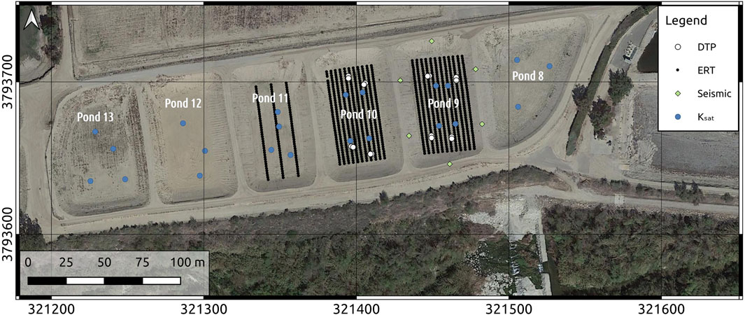
FIGURE 1. Map of the study site showing the investigated infiltration ponds (Ponds 8 to 13 in which EMI data were acquired), the locations of ERT electrodes, infiltration and DTP probes, ambient seismic noise sensors, and measurements of saturated hydraulic conductivity. Aerial photograph obtained from NOAA. Coordinates in NAD83 UTM Zone 11N.

2.2 Electrical resistivity tomography

Electrical Resistivity Tomography (ERT) is a geophysical technique that images the subsurface electrical properties in two, three, or four dimensions (including time). The electrical resistivity of the subsurface is predominantly a function of the lithology, grain size/porosity, water saturation, and pore water chemistry (Archie, 1942). At the study site, groundwater levels were lower than 10 m below ground level (bgl), and hence variations in lithology and grain size are expected to dominate the signal.

ERT data were acquired in 3 of the studied ponds (Uhlemann and Ulrich, 2022). Within ponds 9 and 10, we acquired 3D ERT data, and in pond 11 we acquired a set of 3 parallel ERT profiles. We used an electrode spacing of 1.5 m, and 42 electrodes per profile. For Ponds 9 and 10, 3D data were acquired using a set of 11 and 12 parallel lines, respectively, spaced at 3 m. We acquired dipole-dipole data with dipole lengths a of 1.5, 3.0, 4.5, 6.0, and 7.5 m, and dipole spacing n of 1 to 8a. A full set of reciprocal data were acquired for each profile to assess the data error (Tso et al., 2017). Each electrode location was surveyed using RTK-GPS, with an accuracy of $<$ 2 cm.

The measured resistances need to be inverted to obtain a tomographic resistivity model of the subsurface. Before the inversion, data with reciprocal errors of $>$ 20% were removed, as well as measurements with resistances $<0.005\mathrm{\Omega }$ and $>10\mathrm{\Omega }$. A linear error model was developed based on the measured data of each pond (Figure 2). Errors were generally small $(<1\%)$, and comparable between the ponds. To account for numerical inaccuracies, a modelling error of 1.5% of the measured resistance was applied to the data. These errors were then used in the inversion as data weights. Preprocessing of the data was facilitated using the ResIPy package (Blanchy et al., 2020). The data were inverted using E4D (Johnson et al., 2010) applying L2 model constraints for spatial smoothness, and the inversions converged to χ² = 1, indicating that the model fits the data within their errors. The resulting resistivity models were used to guide intrusive investigation, where two boreholes were drilled in each of ponds 9 and 10. Each borehole extended to about 15 m, with core recovered throughout the length of the borehole.

FIGURE 2

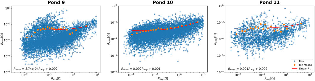
FIGURE 2. Error distribution of the ERT data for each pond, and the linear error models (values shown in the lower left corner of each panel) that were used in the data inversion. Errors are usually small compared to the measured resistances.

2.3 Electromagnetic induction mapping

To rapidly characterize the shallow subsurface properties, an electromagnetic induction (EMI) system, the GF Instruments MiniExplorer 6 L (GF Instruments s.r.o., Brno, Czech Republic), was used. This system weighs only 2 kg, and can easily be walked across a large area sampling the ground at high resolution. The system consists of a transmitter coil and six receiver coils at distances of 0.2, 0.33, 0.5, 0.72, 1.03, and 1.50 m. A primary electromagnetic field at 24.7 kHz created within the transmitter loop, in the presence of conductive material, induces eddy currents in the subsurface, which create a secondary magnetic field that is sensed in the receiver coils and reflects the subsurface electrical properties. To locate measurements, we attached a DGPS (Topcon HIPERV, Livermore, CA, United States) to the logging unit, and recorded both the EMI ground response and the GPS location at 1s intervals. The system was operated using a horizontal coplanar coil orientation, maximizing the effective penetration depth. Data were acquired across 6 ponds (Uhlemann and Ulrich, 2022), Ponds 8 to 13 of the Moorpark Water Reclamation Facility, and data acquisition took about 3 h.

By repeating measurements at the same location at various times, the drift of the system was recorded, but found to be negligible. Data processing included filtering of outliers (data with apparent conductivities ECa $<$ 0 mS/m and ECa $>$ 100 mS/m), averaging of data points that were within a distance of 0.5 m, and removing data points with a standard deviation of more than 5 mS/m within a 1 m radius.

To calibrate the EMI response [which is known to improve the performance of data inversion, McLachlan et al. (2021)], we extracted the ERT resistivity depth-profile at 231 random locations of pond 9, and calculated the EM forward response of those 1D resistivity models. We compared this with the measured EMI data, and used a linear relationship for each coil spacing to calibrate the data (McLachlan et al., 2021). The EM data were then inverted using a cumulative sensitivity approach (McNeill, 1980), which showed comparable results to more exact solutions making use of Maxwell’s equation, but is computationally more efficient. Each EMI sounding was inverted by discretizing the subsurface into 8 layers, with defined thicknesses of 0.2, 0.4, 0.6, 0.8, 1.0, 1.2, 1.5, and an infinite halfspace below. These thicknesses were fixed and we inverted for the resistivity distribution only. We applied an L2 smoothness constraint with a vertical regularization of α = 0.01.

2.4 Saturated hydraulic conductivity measurements

Saturated hydraulic conductivity (K_sat) measurements were made in the top 45–50 cm below the surface of the ponds with a SOILMOISTURE Equipment Corp. Guelph Permeameter. This system is an in-hole constant-head permeameter that can be used to measure the steady-state rate of water infiltration into unsaturated soil in a cylindrical hole, following the Marriotte principle. The measurement is made by filling a cylindrical borehole with a known height of water, maintaining a constant head of water in the borehole, and recording the steady-state rate of water infiltration. By knowing the diameter of the borehole and the height of water, the field saturated hydraulic conductivity can be estimated; note that this represents only the vertical component, i.e., K_sat,z, which we will refer to as K_sat in the following. Within each pond, three to four measurements were conducted, with the locations being guided by the EMI data (Uhlemann and Ulrich, 2022). At each location a 45–50 cm deep, 3” hole was augered, and the test performed with variable heads of 5 and 10 cm. We tried to target locations covering the range of measured electrical properties, however, in areas of particularly sandy material, the shape of the hole could not be sustained throughout the infiltration test, and locations had to be moved. K_sat was calculated for each test following the theory described in Elrick and Reynolds, (2012).

2.5 Groundwater flow modelling

To eventually estimate infiltration rates, we discretize each pond into 1 m × 1 m cells, and calculate a 1D vertical groundwater flow model for each cell, resulting in 2,405 to 3,468 1D flow models per pond. We use Hydrus1D (Šimůnek and Genuchten, 2008), and the python package Phydrus (Collenteur et al., 2021) to automate the model parameterization and simulation. Hydrus1D is solving the Richard’s equation for saturated and non-saturated water flow, and hence provides an adequate choice for the modelling of the vadose zone processes. Unsaturated flow is governed by unsaturated soil hydraulic properties, which are described by van Genuchten, (1980). The model is parameterized in 2.5 cm thick layers to a depth of 250 cm, with K_sat being estimated using a relationship between the measured K_sat and the inverted electrical properties obtained from the calibrated EMI data. Other parameters important for the van Genuchten equation, such as residual soil water content Θ_r = 0.045, saturated soil water content Θ_s = 0.43, soil water retention parameters α = 0.145 1/cm and n = 2.68, and the tortuosity parameter l = 0.5, were taken from literature values for sandy soils. The initial pressure head was set to −500 cm, and the model had a time discretization with a minimum and maximum time step of 10 s and 3 min, respectively. We prescribed a varying pressure head at the surface, resembling a 12 h infiltration period with a head of 50 cm, and defined the lower boundary to be freely draining. This defines a zero pressure head gradient at the lower boundary, which is a valid assumption given the deep groundwater level. The simulation was run for 72 h, and we extracted the infiltration rate at the surface boundary 10 h after start of the infiltration, representing saturated conditions. This model was run for each 1 m × 1 m cell, estimating the infiltration rates for the spatially varying K_sat field of each pond. Note that this is a simplified model that accounts for vertical water flow only, and is not accounting for evapotranspiration or complex subsurface flow patterns.

3 Results

3.1 Electrical resistivity tomography

The resistivity distribution of ponds 9 to 11 show considerable horizontal and vertical variation (Figure 3). In pond 9, a clear boundary can be seen between the low resistivity towards the northern end of the pond compared to the high resistivities of the southern part of the pond. Based on the borehole observations, these changes relate to more clayey and sandy soils that were observed in the northern and southern parts, respectively. The vertical extent of the low resistivity, clayey-dominated fine-grained soils, appears to be limited to 1–2 m depth. This layer is underlain by higher resistivity soils ($>$ 150 Ωm), which are of a more silty-sand texture. The highly resistive, sandy soils in the southern end of pond 9 are underlain by a layer of moderate resistivity (80–200 Ωm), with increasing resistivity with depth. This relates to a silty-sand layer with increasing grain size with depth. Pond 10 shows a continuous, up to 3–5 m thick, surficial layer of high resistivity ($>$ 200 Ωm), which, based on the borehole observations, is interpreted as a continuous layer of sandy soils. Below, resistivities decrease relating to a fining of the subsurface materials, which is more pronounced in the northern part of the pond. Although more uncertain, at a depth of 15–17 m, resistivities increase again, indicating potentially coarser grained material. In the center of pond 10 there is a narrow, low resistivity zone, which is expected to represent silty-clayey soils, which link to the lower resistivities imaged at depth in the northern part of this pond.

FIGURE 3

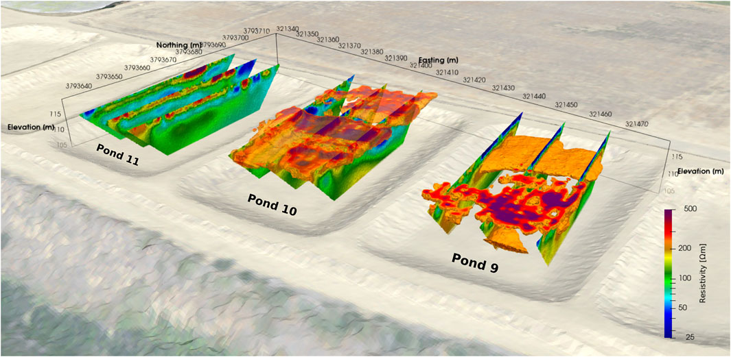
FIGURE 3. Electrical resistivity models obtained from the ERT data inversion. Shown are slices through the 3D models for ponds 9 and 10, and the 2D profiles that were acquired in pond 11. For ponds 9 and 10, resistivities $>$ 200 Ωm are shown in 3D, which represent a sandy layer. Note that at the northern part of pond 9, this layer is overlain by a thick layer of low resistivity sediments. Inversions converged to χ² = 1.

The resistivity data of pond 11 shows a resistive ($>$ 200 Ωm) shallow anomaly. This channel feature appears to widen towards pond 12 and is less than 2 m deep. In general, the resistivity data of pond 11 shows a thin ($<$1 m), high resistivity layer, which is interpreted to be a sandy soil, overlaying a less resistive layer ($<$60 Ωm) of 1–2 m thickness. Below this layer, resistivities increase again to values $>$ 100 Ωm. This can be interpreted as a sequence of sandy soils overlaying silty-sand above a sandy layer.

3.2 Electromagnetic induction mapping

Apparent conductivities recorded using the EMI instruments show that soil electrical conductivities vary spatially and with depth in each pond (Figure 4). The apparent electrical conductivities (ECa) range from close to zero to 50 mS/m. Very low conductivity ($<$ 10 mS/m) is observed across all ponds in Figure 4A for an apparent depth of 0.3 m, except in the northern parts of ponds 8 and 9, where conductivities up to 35 mS/m were recorded. These low ECa relate to very sandy soils that were observed in the southern parts of ponds 8 and 9, and throughout ponds 10 to 13. The higher ECa relate to soils that were observed to be rich in clay and silt. For all ponds ECa increases with increasing depth, indicating an increase in soil moisture with depth. Data from deeper apparent depth show more distinct and spatially continuous subsurface features. A well-defined, low conductivity feature is observed trending northeast-southwest across pond 10 (north side) into 11, and on into pond 12 (red zone middle of pond) passing through the southeast corner of pond 13. This is a distinct feature for investigation depths of 0.5–1.6 m, but has only a faint signature for an investigation depth of 2.3 m. A similar, but larger, low conductivity feature can be seen with the same orientation within the southern parts of ponds 8 and 9. Because of the large variability between ponds 9 and 10, which show very different electrical signatures, these two were chosen for the 3D ERT data acquisition and were eventually used to calibrate the EMI data. Figure 5 shows the final misfit of the inversion between modeled and observed data and highlights the importance of this calibration. While in the uncalibrated case there is an offset between observed and modeled response that varies for each coil spacing, this offset is eliminated by the calibration and the data falls almost perfectly along the 1:1 line. This improvement also results in a better data fit between the observed and modelled data, where the RRMSE error decreases from 0.16 to 0.02%.

FIGURE 4

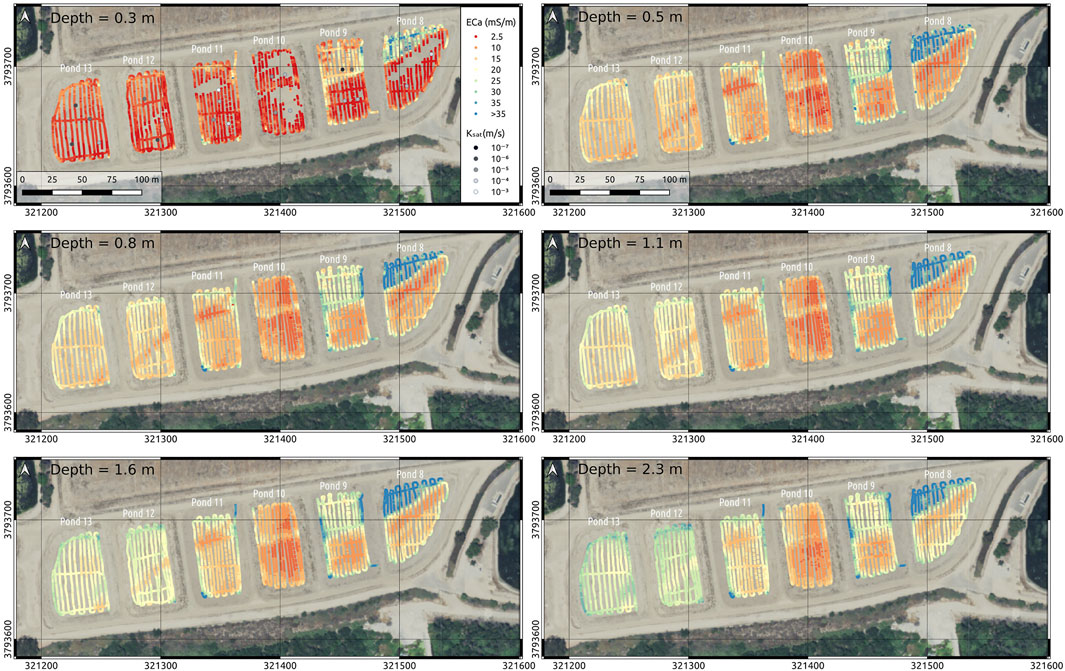
FIGURE 4. Apparent conductivity at 0.3–2.3 m depth measured using EMI. Note the differences in pond 8 and 9 where low and high conductivities are clearly separated. Shown are also the saturated hydraulic conductivities measured with the Guelph permeameter in the top left image (ECa at 0.3 m depth).

FIGURE 5

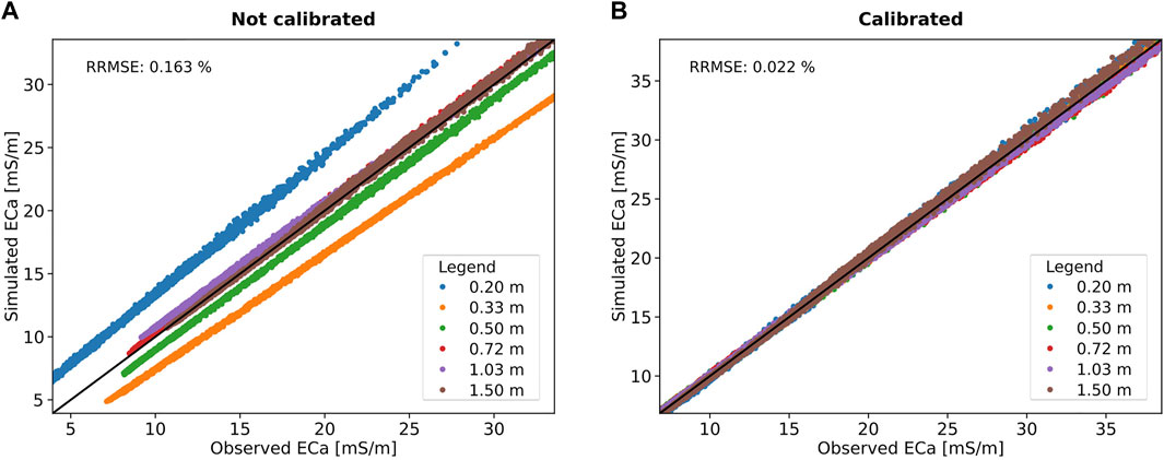
FIGURE 5. Misfit between modelled and measured electrical conductivity after inversion for the uncalibrated (A) and ERT-calibrated EMI data (B). Note the much smaller misfit for all coil spacings in the calibrated case.

The inverted EMI resistivity models (Figure 6) show the same observations for ponds 9 to 11 as presented for the ERT data. For pond 8, shallow depths are characterized by a conductive northern part and a resistive southern part. This distinct characteristic continues throughout the depth of investigation of the EMI (≈2.5 m), with slightly decreasing resistivities with depth. In contrast, for ponds 12 and 13, a shallow ($<$ 1 depth), highly resistive layer ($>$ 150 Ωm), overlays a considerably less resistive layer ($<$ 50 Ωm). This indicates that ponds 12 and 13 are characterized by a thin sandy soil cover, with likely more silty-clayey material below.

FIGURE 6

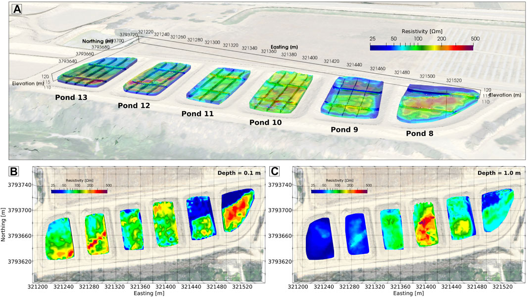
FIGURE 6. Inverted resistivity models. (A) 3D view of Ponds 8 to 13., (B) horizontal slice at 0.1 m depth, (C) horizontal slice at 1.0 m depth. (B) and (C) capture the lateral and vertical soil heterogeneity and identify bounds of the fines dominated, low hydraulic conductivity (blue) and coarser, high hydraulic conductivity (yellow-red) soils.

From those data, and relating high resistivity with high hydraulic conductivity and vice versa, we expect pond 10 to have the highest recharge potential, as this pond shows the highest resistivities throughout (mean resistivity of 152.3 Ωm). Even though ponds 8 and 9 have a shallow low resistivity layer in the northern part, which is likely of low hydraulic conductivity, this layer is thin, and below resistivities are comparably high, resulting in comparably high average resistivities (75.2 and 79.9 Ωm, respectively). Similarly, pond 11 shows moderate resistivities throughout (average of 91.4 Ωm). Hence, we expect ponds 8, 9, and 11 to have moderate recharge potential. Ponds 12 and 13, even though characterized by a thin resistive soil layer, which is likely high in sand content, have likely low recharge potential because of the low resistivity layer that underlays this thin top layer (average resistivities of 66.9 and 50.0 Ωm, respectively). This indicates a trend of decreasing electrical resistivity towards the western side of the facility.

3.3 Saturated hydraulic conductivities

Similar to the ERT and EMI data, the measured saturated hydraulic conductivities (Figure 7) show variable values for each pond, with pond 9 showing the biggest range with K_sat varying between 6.49 ⋅ 10^–7 m/s and 9.9 ⋅ 10^–5 m/s (average of K_sat = 3.8 ⋅ 10–5 m/s). The largest average K_sat values were observed for ponds 11 and 8 (1.33 ⋅ 10^–4 m/s and 7.04 ⋅ 10^–5 m/s, respectively), followed by pond 10 (3.19 ⋅ 10^–5 m/s). Ponds 12 and 13 showed the smallest average K_sat (6.61 ⋅ 10^–6 m/s and 4.23 ⋅ 10^–6 m/s, respectively). Since the average of each pond is defined by 3–4 sampling points only, the measured values and distributions may not represent the true heterogeneity of each pond, but these values provide some insight into their distribution. Nevertheless, the comparably small variability of pond 10 highlights again the relatively homogeneous conditions of this pond, and the rather poor potential recharge performance of ponds 12 and 13, where the lowest K_sat were measured. Similarly to the electrical resistivities, this indicates a trend of decreasing hydraulic conductivity towards the western ponds.

FIGURE 7

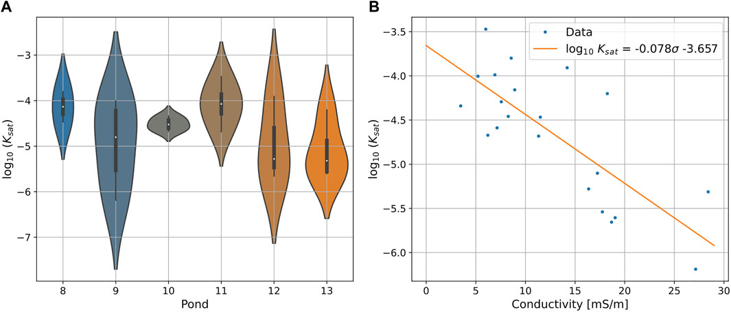
FIGURE 7. (A) Distributions of saturated hydraulic conductivity for each pond. (B) Linear relationship linking electrical conductivity to hydraulic conductivity.

To provide an estimate of the spatial heterogeneity of K_sat throughout the ponds, we established a relationship between measured K_sat and the electrical conductivity obtained from EMI. This is a valid approach since the electrical conductivity of soils is known to be a function of grain size (Banton et al., 1997; Uhlemann et al., 2017), which in turn relates to the hydraulic conductivity (Rosas et al., 2014). A linear relationship between conductivity and K_sat was found to fit the data reasonably well (R² = 0.58, Figure 7). K_sat can be estimated from the electrical conductivity (σ) through:

${\log }_{10}{K}_{\mathit{sat}}=-0.078\sigma -3.657(1)$

Using this relationship, we translated the measured 3D models of electrical conductivity into K_sat (Figure 8). At 0.1 m depth, throughout all ponds K_sat is relatively high with values mostly $>10^{-5}$, with the only exception being in the northern part of ponds 8 and 9, where K_sat < 10^–6. At 1 m depth, more spatial variability can be observed, with ponds 9, 10, and 11 showing K_sat > 10^–5, and ponds 8, 12, and 13 showing smaller values of K_sat < 10^–5. The results indicate a trend of decreasing K_sat at depth towards the west. To assess the prediction accuracy, we estimated K_sat for each of the Guelph tests and compared them to the measured values (Figure 9). The relationship used to estimate K_sat from the electrical conductivity distribution usually yields estimates that are within the same order of magnitude than the measured values (R² = 0.63), and generally recover the trend within each pond.

FIGURE 8

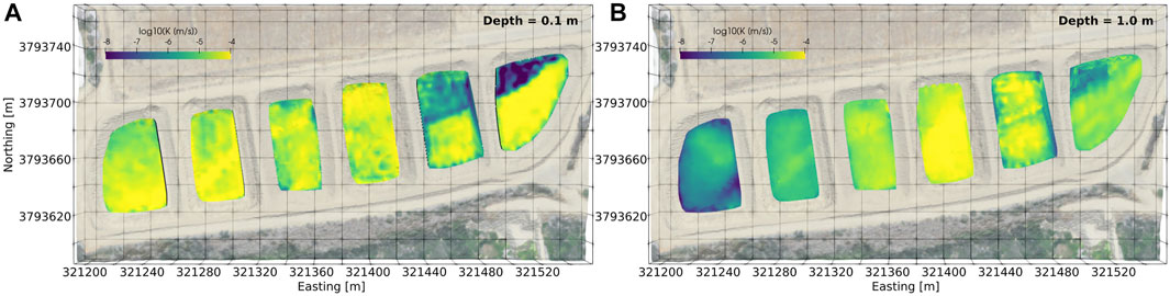
FIGURE 8. Horizontal slices through the derived 3D hydraulic conductivity model at (A) 0.1 m depth and (B) 1.0 m depth.

FIGURE 9

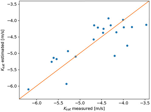
FIGURE 9. Measured and estimated saturated hydraulic conductivity. The estimated data usually falls within the same order of magnitude than the measured data and has a R² = 0.63.

3.4 Estimated infiltration rates

To assess potential infiltration rates, we used the derived spatial distribution of hydraulic conductivities (Figure 8) to parameterize a simple 1D vertical groundwater flow model. Each pond, we subdivided into 1 m × 1 m grid cells, and we extracted K_sat for each of those cells at 0.5 m intervals from 0 to 2.5 m depth. Recharge was simulated by applying a 0.5 m head to this area over a period of 12 h. The model itself was run for a duration of 72 h. We extracted the infiltration rate at each surface cell 10 h after start of the infiltration to ensure saturated conditions.

Similar to the K_sat observations, ponds 8 and 9 show a clear division in potential infiltration rates (Figure 10), with the northern parts showing small values (close to zero cm/h), and the southern part having larger values ($>$ 6 cm/h). On average, ponds 8 and 9 have an estimated infiltration rate of 3.3 and 2.9 cm/h. The largest infiltration rates are estimated for pond 10, which has an average of 12.4 cm/h and values exceeding 26 cm/h. Pond 11 is estimated to have a mean infiltration rate of 5.1 cm/h. The smallest infiltration rates were estimated for ponds 12 an 13, with 2.1 cm/h and 0.5 cm/h, respectively.

FIGURE 10

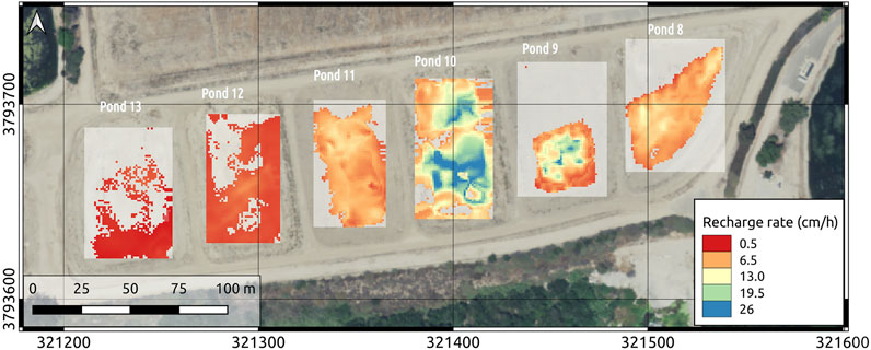
FIGURE 10. Infiltration rate estimated using 1D vertical groundwater flow models for 1 m × 1 m cells parameterized based on the hydraulic conductivity estimated from the EMI data (Figure 8). Note, grey zones within the ponds indicate areas of estimated infiltration rates $<$ 0.5 cm/h.

4 Discussion

Our results show the benefit of using geophysical investigations to rapidly assess the hydrogeological conditions of recharge ponds. The resistivity distributions of ERT and EMI show low values in the shallow subsurface of the northern part of ponds 8 and 9, and decreasing values with depth for ponds 12 and 13. Measurements of K_sat show similar variability, with pond 10 and 11 showing the largest values, while ponds 12 and 13 show the smallest hydraulic conductivities. Using simple 1D groundwater flow simulations, we can relate the distribution of hydraulic conductivities to potential infiltration rates, and show that the ponds that are characterized by higher resistivity, and thus higher hydraulic conductivity, also have higher infiltration rates. Here, infiltration rates vary from $<0.5$ cm/h to $>25$ cm/h. Particularly for pond 9, which is characterized by a shallow ($<$ 1 m thick) low resistivity layer of low hydraulic conductivity. Such a thin surficial layer, which is known to build up due to settlement of fines during operation of such recharge ponds, can impede high infiltration and hence recharge rates and thus lower the performance of those ponds. The data acquired here can help to improve the management of these ponds. In this case, removal of this layer could help to increase infiltration and recharge rates. We quantified the impact of such an operation by removing the low hydraulic conductivity surficial layer in the 1D groundwater flow model, and replaced the values with random values sampled from a normal distribution that describes K_sat observed in the southern part of this pond. While the observed data (i.e., including the surficial low hydraulic conductivity layer) shows very low infiltration rates in the northern part of the pond, the simulated intervention increases the infiltration rate significantly from 2.9 to 7.9 cm/h. Assuming that the entire pond would be used for recharge, this would result in an increase in infiltration during a single day (24 h) from 2,186 m³ to 6,224 m³. These values are also in agreement with real infiltration rates, where the pond was filled with 793 m³ of recycled water during a separate experiment, which infiltrated in less than 24 h. A similar experiment was also conducted in pond 10, which has an estimated infiltration volume of 8,590 m³/day, but in this pond, the pumps could not supply sufficient water to actually fill the pond. This highlights the higher infiltration rate of pond 10 compared to pond 9, and provides further support for the validity of our results. These infiltration volumes are in stark contrast to the estimated volumes per day for ponds 12 and 13, which are only 1,278 m³ and 354 m³. Since the limiting factor of those ponds is the shallow, but thick, small hydraulic conductivity layer, installation of dry wells in those ponds could facilitate the movement of water into the deeper aquifer units, which, based on the ERT results, seem to be dipping deeper from the eastern to the western side of the facility.

Although we could not directly measure the infiltration rate of these ponds, the presented approach shows considerable variability throughout the facility, which is in agreement with observations of recharge activities. Here, data acquisition of the ERT, EMI, and hydraulic conductivity took less than 4 days for a crew of two people. With this effort, we could provide a quantitative assessment of infiltration rates for six different ponds, and propose detailed management activities that could increase the infiltration volume of a particular pond by 284%.

Here, we translate the inverted 3D resistivity models into 3D distributions of vertical saturated hydraulic conductivity, based on a linear relationship between the electrical conductivity (i.e., the inverse of the resistivity) and K_sat. While the linear fit is acceptable, additional measurements of K_sat at different locations and depths would certainly help in providing a more robust relationship. In this analysis, we are neglecting the effects of anisotropic hydraulic conductivity, and hence only consider vertical water movements. If the horizontal hydraulic conductivity would be considerably larger than the vertical, complex groundwater pathways may also contribute to recharge. Additionally, the K_sat data may not necessarily truly represent the range of hydraulic conductivities of the ponds, as measurements could not be made in the most sandy locations, as the boreholes were collapsing and prevented measurements. Using field determined petrophysical relationships to translate imaged electrical properties to hydraulic conductivity assumes that there is a direct relationship between these values. While both electrical and hydraulic conductivity are governed by the soil texture (Durner, 1994; Domsch and Giebel, 2004), other factors such as the clay content may affect the electrical conductivity, leading to non-linear and more complex relationships between the two values. While this is not the case at this study site, it may be a limiting factor at other sites. Additionally, here we assume that the inversion recovers the true resistivity distribution throughout the model space. Yet, the inversion makes use of smoothness constraints, and particularly with increasing depth, the sensitivity of the measurements decreases, resulting in a smooth representation of the resistivity distribution. This may affect the translation of the inverted resistivity model, which is most likely underestimating the true resistivity distribution, into K_sat (Day-Lewis et al., 2005), and we are hence likely underestimating K_sat at depth. Since we only consider the upper 2.5 m for the 1D groundwater flow models, the impact of that should be limited.

While the presented approach should be applicable to characterize and estimate hydrological properties of other recharge facilities, the linear relationship (Eq. 1) between the electrical conductivity and K_sat is likely site-specific, and should be obtained for each site. Nevertheless, as shown here, such an integrated approach of geophysical and hydrological measurements can provide valuable data for managers of such facilities, and may increase performance, while at the same time lowering maintenance costs through detailed information to design improvement strategies.

5 Conclusion

Managed aquifer recharge is a technology that can enhance groundwater recharge, thereby reducing the stress that is put on aquifers due to increased groundwater extraction and changing precipitation patterns. However, we are lacking approaches that can quantify recharge contributions, which can directly aid in the management of these facilities. Here, we introduce a workflow that combines electrical and electromagnetic geophysics with direct measurements of saturated hydraulic conductivity. Through establishing a linear relationship between hydraulic conductivity and electrical properties of the ground, we can use geophysical imaging methods to map the 3D distribution of hydraulic conductivity and use the distributed values to parameterize hydrological models to estimate infiltration rates. We show that the electrical and hydraulic properties vary considerably throughout the investigated recharge facility, showing infiltration rates of $<$ 0.5 to $>$ 25 cm/h. This results in potential daily infiltration volumes of 354 m³ for the least efficient to 8,590 m³ for the most efficient pond. Using the model, we can also assess the impact of management activities, and show that the removal of a shallow, low hydraulic conductivity layer could result in a 284% increase in infiltration volume.

The presented approach is cost-efficient, and transferable to other sites, and can provide a workflow to rapidly assess potential infiltration rates and volumes for recharge facilities. We show that this approach can also be used to assess the impact of management activities, and by repeating the presented approach over time, it could also be used to monitor the performance and design detailed management activities. To gain detailed information about the actual recharge processes, full-scale recharge experiments were conducted in ponds 9 and 10 and monitored using a range of sensing techniques. The results of those experiments highlight the importance of preferential flow paths that were identified in this characterization study, and will be the focus of a follow-on paper.

Data availability statement

The datasets presented in this study can be found in online repositories. The names of the repository/repositories and accession number(s) can be found below: http://www.hydroshare.org/resource/74650ddf75d946fdae57956045490a1c.

Author contributions

SU, CU, PF, and JK contributed to conception and design of the study. CU, JK, and JP managed the project, as well as coordinated on COVID-19 safety requirements. SU and CU acquired and analyzed the geophysical and hydraulic data. SU wrote the first draft of the manuscript. All authors contributed to manuscript revision, read, and approved the submitted version.

Funding

Funding for this project was provided through the Metropolitan Water District of Southern California’s Future Supply Actions Funding Program under Agreement Number 188682.

Acknowledgments

The authors would like to acknowledge our partners at the Metropolitan Water District, Calleguas Municipal Water District and VCWWD for their efforts in making this project successful despite the challenges encountered during the COVID-19 Pandemic.

Conflict of interest

The authors declare that the research was conducted in the absence of any commercial or financial relationships that could be construed as a potential conflict of interest.

Publisher’s note

All claims expressed in this article are solely those of the authors and do not necessarily represent those of their affiliated organizations, or those of the publisher, the editors and the reviewers. Any product that may be evaluated in this article, or claim that may be made by its manufacturer, is not guaranteed or endorsed by the publisher.

References

Archie, G. E. (1942). The electrical resistivity log as an aid in determining some reservoir characteristics. Trans. AIME 146, 54–62. doi:10.2118/942054-g

CrossRef Full Text | Google Scholar

Arias, P., Bellouin, N., Coppola, E., Jones, R., Krinner, G., Marotzke, J., et al. (2021). “Technical summary,” in Climate change 2021: The physical science basis. Contribution of working group I to the sixth assessment report of the intergovernmental panel on climate change. Editors V. Masson-Delmotte, P. Zhai, and A. Pirani (Cambridge University Press).

Google Scholar

Banton, O., Cimon, M.-A., and Seguin, M.-K. (1997). Mapping field-scale physical properties of soil with electrical resistivity. Soil Sci. Soc. Am. J. 61, 1010–1017. doi:10.2136/sssaj1997.03615995006100040003x

CrossRef Full Text | Google Scholar

Behroozmand, A. A., Auken, E., and Knight, R. (2019). Assessment of managed aquifer recharge sites using a new geophysical imaging method. Vadose zone J. 18, 1–13. doi:10.2136/vzj2018.10.0184

CrossRef Full Text | Google Scholar

Binley, A., Hubbard, S. S., Huisman, J. A., Revil, A., Robinson, D. A., Singha, K., et al. (2015). The emergence of hydrogeophysics for improved understanding of subsurface processes over multiple scales. Water Resour. Res. 51, 3837–3866. doi:10.1002/2015WR017016

PubMed Abstract | CrossRef Full Text | Google Scholar

Blanchy, G., Saneiyan, S., Boyd, J., McLachlan, P., and Binley, A. (2020). ResIPy, an intuitive open source software for complex geoelectrical inversion/modeling. Comput. Geosciences 137, 104423. doi:10.1016/j.cageo.2020.104423

CrossRef Full Text | Google Scholar

[Dataset] Collenteur, R., Brunetti, G., and Vremec, M. (2021). Phydrus: Python implementation of the HYDRUS-1D unsaturated zone model. Version 0.2.0

Google Scholar

Day-Lewis, F. D., Singha, K., and Binley, A. M. (2005). Applying petrophysical models to radar travel time and electrical resistivity tomograms: Resolution-dependent limitations. J. Geophys. Res. 110, B08206. doi:10.1029/2004JB003569

CrossRef Full Text | Google Scholar

Domsch, H., and Giebel, A. (2004). Estimation of soil textural features from soil electrical conductivity recorded using the EM38. Precis. Agric. 5, 389–409. doi:10.1023/B:PRAG.0000040807.18932.80

CrossRef Full Text | Google Scholar

Durner, W. (1994). Hydraulic conductivity estimation for soils with heterogeneous pore structure. Water Resour. Res. 30, 211–223. doi:10.1029/93WR02676

CrossRef Full Text | Google Scholar

Elrick, D. E., and Reynolds, W. D. (2012). Infiltration from constant-head well permeameters and infiltrometers. Adv. Meas. Soil Phys. Prop. Bringing Theory into Pract. 30, 1–24. doi:10.2136/sssaspecpub30.c1

CrossRef Full Text | Google Scholar

FCGMA (2016). Annual report for calendar year 2016. Tech. rep. Ventura, CA: Fox Canyon Groundwater Management Agency.

Google Scholar

Füssel, H. H.-M., Jol, A., Kurnik, B., Hemming, D., and Hildén, M. (2012). Climate change, impacts and vulnerability in europe 2012: An indicator-based report, 12. Copenhagen: EEA - European Environment Agency.

Google Scholar

Hanson, R., Martin, P., and Koczot, K. (2003). Simulation of ground-water/surface-water flow in the Santa Clara-Calleguas ground-water basin, Ventura County, California. Tech. rep. Sacramento, CA: USGS.

Google Scholar

Johnson, T. C., Versteeg, R. J., Ward, A., Day-Lewis, F. D., and Revil, A. (2010). Improved hydrogeophysical characterization and monitoring through parallel modeling and inversion of time-domain resistivity and induced-polarization data. Geophysics 75, WA27–WA41. doi:10.1190/1.3475513

CrossRef Full Text | Google Scholar

Kang, S., Knight, R., Greene, T., Buck, C., and Fogg, G. (2021). Exploring the model space of Airborne electromagnetic data to delineate large-scale structure and heterogeneity within an aquifer system. Water Resour. Res. 57, 1–31. doi:10.1029/2021WR029699

CrossRef Full Text | Google Scholar

Kinzelbach, W., Bauer, P., Siegfried, T., and Brunner, P. (2003). Sustainable groundwater management — Problems and scientific tools. Episodes 26, 279–284. doi:10.18814/epiiugs/2003/v26i4/002

CrossRef Full Text | Google Scholar

Knight, R., Smith, R., Asch, T., Abraham, J., Cannia, J., Viezzoli, A., et al. (2018). Mapping aquifer systems with Airborne electromagnetics in the central valley of California. Groundwater 56, 893–908. doi:10.1111/gwat.12656

PubMed Abstract | CrossRef Full Text | Google Scholar

Mawer, C., Parsekian, A., Pidlisecky, A., and Knight, R. (2016). Characterizing heterogeneity in infiltration rates during managed aquifer recharge. Groundwater 54, 818–829. doi:10.1111/gwat.12423

CrossRef Full Text | Google Scholar

McLachlan, P., Blanchy, G., and Binley, A. (2021). EMagPy: Open-source standalone software for processing, forward modeling and inversion of electromagnetic induction data. Comput. Geosci. 146, 104561–104632. doi:10.1016/j.cageo.2020.104561

CrossRef Full Text | Google Scholar

McNeill, J. (1980). Electromagnetic terrain conductivity measurement at low induction numbers. Tech. Rep. Ontario: Geonics Limited.

Google Scholar

Nouveau, M., Grandjean, G., Leroy, P., Philippe, M., Hedri, E., and Boukcim, H. (2016). Electrical and thermal behavior of unsaturated soils: Experimental results. J. Appl. Geophys. 128, 115–122. doi:10.1016/j.jappgeo.2016.03.019

CrossRef Full Text | Google Scholar

Rodell, M., Famiglietti, J. S., Wiese, D. N., Reager, J. T., Beaudoing, H. K., Landerer, F. W., et al. (2018). Emerging trends in global freshwater availability. Nature 557, 651–659. doi:10.1038/s41586-018-0123-1

PubMed Abstract | CrossRef Full Text | Google Scholar

Rosas, J., Lopez, O., Missimer, T. M., Coulibaly, K. M., Dehwah, A. H., Sesler, K., et al. (2014). Determination of hydraulic conductivity from grain-size distribution for different depositional environments. Groundwater 52, 399–413. doi:10.1111/gwat.12078

PubMed Abstract | CrossRef Full Text | Google Scholar

Scanlon, B. R., Faunt, C. C., Longuevergne, L., Reedy, R. C., Alley, W. M., McGuire, V. L., et al. (2012). Groundwater depletion and sustainability of irrigation in the US high plains and central valley. Proc. Natl. Acad. Sci. U. S. A. 109, 9320–9325. doi:10.1073/pnas.1200311109

PubMed Abstract | CrossRef Full Text | Google Scholar

Sendrós, A., Himi, M., Lovera, R., Rivero, L., Garcia-Artigas, R., Urruela, A., et al. (2020). Geophysical characterization of hydraulic properties around a managed aquifer recharge system over the llobregat river alluvial aquifer (barcelona metropolitan area). Water 12, 3455. doi:10.3390/w12123455

CrossRef Full Text | Google Scholar

Šimůnek, J., and Genuchten, M. T. (2008). Modeling nonequilibrium flow and transport processes using HYDRUS. Vadose zone J. 7, 782–797. doi:10.2136/vzj2007.0074

CrossRef Full Text | Google Scholar

Singh, A., Panda, S. N., Uzokwe, V. N., and Krause, P. (2019). An assessment of groundwater recharge estimation techniques for sustainable resource management. Groundw. Sustain. Dev. 9, 100218. doi:10.1016/j.gsd.2019.100218

CrossRef Full Text | Google Scholar

Sterrett, R. J. (1985). Advanced soil mechanics. Eos Trans. AGU. 66, 714. doi:10.1029/EO066i042p00714-02

CrossRef Full Text | Google Scholar

SWRCB (2014). Sustainable groundwater management act 2014. Sacramento: State Water Resources Control Board.

Google Scholar

Tso, C.-h. M., Kuras, O., Wilkinson, P. B., Uhlemann, S., Chambers, J. E., Meldrum, P. I., et al. (2017). Improved characterisation and modelling of measurement errors in electrical resistivity tomography (ERT) surveys. J. Appl. Geophys. 146, 103–119. doi:10.1016/j.jappgeo.2017.09.009

CrossRef Full Text | Google Scholar

Uhlemann, S., Kuras, O., Richards, L. A., Naden, E., and Polya, D. A. (2017). Electrical resistivity tomography determines the spatial distribution of clay layer thickness and aquifer vulnerability, Kandal Province, Cambodia. J. Asian Earth Sci. 147, 402–414. doi:10.1016/j.jseaes.2017.07.043

CrossRef Full Text | Google Scholar

[Dataset] Uhlemann, S., and Ulrich, C. (2022). Hydrogeophysical characterization data of the Moorpark reclamation facility. Available at: http://www.hydroshare.org/resource/74650ddf75d946fdae57956045490a1c.

Google Scholar

van Genuchten, M. T. (1980). A closed-form equation for predicting the hydraulic conductivity of unsaturated soils. Soil Sci. Soc. Am. J. 44, 892–898. doi:10.2136/sssaj1980.03615995004400050002x

CrossRef Full Text | Google Scholar

VCWPD (2015). 2015 annual report of groundwater conditions. Tech. rep. Ventura County Watershed Protection District.

Google Scholar