 Weijin Xu
 Xuejing Li
- Institute of Geophysics, China Earthquake Administration, Beijing, China
The characteristics of seismic temporal distribution represent an important basis for earthquake prediction and seismic hazard analysis. In this paper, based on the seismic catalogs in Taiwan, and using Poisson (exponential distribution), Gamma, Lognormal, Weibull, and Brownian passage time distributions as target models, we adopt the maximum likelihood method for estimating model parameters. The optimal model for describing the temporal distribution of earthquakes in Taiwan is determined according to the Akaike Information Criterion (AIC), Bayesian Information Criterion (BIC), K-S test, Chi-square test, and coefficient of determination R2 results. The results show that for moderate-strong earthquakes events (MW < 7.0), the Gamma distribution model can well describe the temporal distribution characteristics of earthquakes, while large earthquakes (MW ≥ 7.0) can be described entirely by exponential distribution. In addition, the temporal correlation between earthquakes is also examined through diffusion entropy analysis. The results show that seismic activity features temporal correlation, and earthquakes with relatively small magnitude (MW < 7) are affected by larger events (MW ≥ 7.0), thus suggesting long-term memory in time. In this study, the probability of the occurrence of a major earthquake in Taiwan is also calculated. The results show that the probability of an MW ≥ 7.0 earthquake in Taiwan in the next 10 years reaches 91.3%. The results may be used to inform the selection of seismic time distribution models and the calculation of seismic activity parameters in earthquake prediction and seismic hazard calculation, and hold scientific significance for understanding the mechanism of earthquake genesis.
1 Introduction
The temporal distribution models of earthquakes represent an important theoretical basis for earthquake prediction and seismic hazard analysis. Currently, it is widely assumed in probabilistic seismic hazard analysis and earthquake prediction that the temporal occurrence of earthquakes follows Poisson distribution. This means that earthquake occurrences are mutually unrelated overtime, that is, they will neither be affected by previous events nor affect subsequent events. Time-independent models include Poisson, double Poisson, piecewise Poisson, and renewal models (Cornell, 1968; Gardner, 1974; Schwartz and Coppersmith, 1984; Hu, 1990; Console et al., 2003), among which the Poisson model is widely used in seismology and engineering seismology. A lot of statistical tests have been conducted on whether the temporal distribution of earthquakes conforms to the Poisson model (Gardner, 1974; Bufe and Perkins, 2005; Michael, 2011; Parsons and Geist, 2012; Shearer and Stark 2012). In many countries, the Poisson model is currently used in seismic hazard mapping and analysis (such as Cornell, 1968; Petersen et al., 2014).
In contrast to time-independent models, time-dependent models are used to describe the temporal distribution of earthquakes. In recent decades, scientists have used earthquake catalogs in different regions to empirically investigate the temporal dependence of earthquakes, and found that in many cases, the temporal occurrences of earthquakes do not follow the Poisson distribution, while time-dependent models are able to describe their temporal distribution more accurately (Utsu, 1984; Nishenko and Buland, 1987; Ogata, 1998; Tripathi, 2006; Sharma and Kumar, 2010). Scientists have proposed to describe the temporal distribution of earthquakes by using Gamma, Lognormal, Weibull and Brownian passage time functions (Utsu, 1984; Matthews et al., 2002; Tripathi, 2006; Pasari and Dikshit, 2015; Pasari and Dikshit, 2018; Bajaj and Sharma, 2019), which have provided important theoretical ground for earthquake prediction and seismic hazard analysis.
In addition, the Epidemic Type Aftershock Sequence (ETAS) model has also been widely used to study the temporal and spatial distribution of earthquakes in recent years (Ogata, 1998; Zhuang et al., 2005; Ogata and Zhuang, 2006). The ETAS model has achieved considerable success in describing earthquakes and their aftershocks, and in aftershock prediction. However, for seismic hazard analysis, scientists have paid more attention to the temporal distribution characteristics of main shocks (Michael, 2011; Beroza, 2012; Daub et al., 2012; Shearer and Stark, 2012). In fact, in the ETAS model, background earthquakes are sometimes still regarded as following the Poisson distribution (Zhuang et al., 2005; Lombardi and Marzocchi, 2007). When applying the ETAS model to probabilistic seismic hazard analysis, Šipčić et al. (2022) identified the characteristics of the temporal changes of background seismicity in the ETAS model as a key area for future research, which suggests that studying the temporal distribution of main shocks will also contribute to the effective use of the ETAS model.
In the present study, based on the earthquake catalogs recorded by relatively dense earthquake networks in Taiwan, and using Poisson (exponential distribution), Gamma, Lognormal, Weibull and Brownian passage time as target models, we regressed the parameters of each model and selected the optimal model for describing the temporal distribution of seismicity using the Akaike information criterion (AIC), the Bayesian information criterion (BIC) and the Kolmogorov-Smirnov test (K-S test). Based on the above models, we calculated the occurrence probability of large earthquakes in Taiwan. The temporal correlation of earthquakes in Taiwan and its surrounding areas was also studied using Diffusion Entropy Analysis (DEA). The results of this paper may provide theoretical basis for the selection of temporal distribution models and the calculation of seismicity parameters in seismic hazard analysis in the Taiwan area.
2 Data and methods
2.1 Earthquake catalogs
The earthquake catalogs used in this study are obtained from the weather bureau of the Taiwan area (Figure 1). The earthquake catalogs contain over 14,700 seismic events with ≤40 km depth and M ≥ 4.0 magnitude from 1900 to 2020. With the average crustal depth in Taiwan being about 40 km (Yeh and Tsai 1981), the catalogs represent a record of shallow earthquakes in Taiwan. Taiwan scholars have revised local earthquake catalogs in seismicity analysis and seismic hazard calculations (e.g., Cheng et al., 2010; Chen et al., 2013; Chen and Chang, 2017), ensuring that important parameters such as time, location and magnitude in the earthquake catalogs are reliable and can be used for analysis in the present study. In the study, we also used the ANSS Comprehensive Earthquake Catalog (ComCat) of the US Geological Survey, which contains the major events in the world with moment magnitude. We used Werner and Sornette (2008)’s method to determine whether the seismic events recorded by the weather bureau of the Taiwan area are the same as those in the ANSS ComCat catalogs, and determined their moment magnitudes. For events that are not listed in ANSS ComCat catalog and have no moment magnitude, the conversion relationship established by Chen and Tsai (2008) was used to turn the magnitude into moment magnitude.
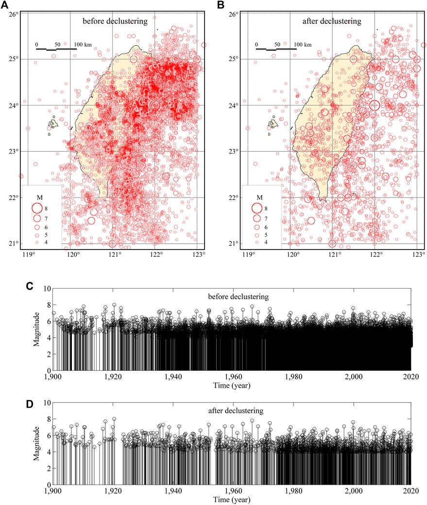
FIGURE 1. Temporal and spatial distribution of earthquakes in Taiwan. (A,B) are the seismic spatial distribution maps before and after declustering, respectively. (C,D) are the magnitude—time distribution before and after declustering, respectively.
In this study, it is necessary to remove the aftershocks from the earthquake catalogs to analyze the temporal statistics of main shocks, for which many methods are currently available. Among them, the traditional space-time window (Gardner, 1974) gives a certain window of time and distances according to main shock magnitude, and events within the window are regarded as aftershocks. Though it is a simple method for aftershock identification, the space-time window requires the provision of corresponding space-time window parameters according to the tectonic features of different regions. Zhuang et al. (2002) proposed a stochastic declustering approach based on the ETAS model. Despite its high efficiency in declustering, it requires estimating the parameters in the ETAS model in advance, which may be difficult in areas with relatively few or incomplete catalogs. In addition, the method requires massive calculations. Moreover, some scholars put forward the nearest neighbor distance method for aftershock deletion (Baiesi and Paczuski, 2004). In this paper, we used the space-time window of Gardner (1974), which is widely used in seismicity analysis and seismic hazard analysis at present (Daub et al., 2012; Shearer and Stark, 2012; Petersen et al., 2014), to remove aftershocks from the catalogs in Taiwan. The time-space window parameters used by Chen et al. (2013) and Obi et al. (2017) were adopted. Figure 1 is the spatial distribution map (Figures 1A, B) and magnitude-time distribution map (Figures 1C, D) of earthquakes before and after removing aftershocks, which shows greatly reduced seismic data after removal. As different aftershock declustering methods will lead to biases in model parameters estimation (Taroni & Akinci, 2021), we also used Reasenberg (1985)’s method to decluster the catalogs to ensure the robustness of the results. As Table 1 shows, Reasenberg (1985)’s declustering method retained more seismic events.
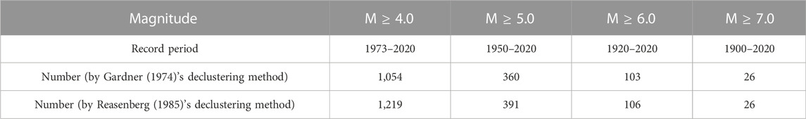
TABLE 1. Time periods of complete earthquake records in Taiwan area.
The completeness of catalogs, which refers to complete records of earthquakes with a certain magnitude or above starting from a certain year, might also affect results in significant ways. In this paper, we considered the analysis results of Chen et al. (2013), Wang et al. (2016), and Chen and Chang (2017) on the completeness of earthquake catalogs in Taiwan (Table 1), among which the complete records of earthquakes of M4 or above started from 1973, and that of M7.0 or above started from 1900.
2.2 Statistical model of time intervals of earthquake occurrence and goodness-of-fit (GOF) test
In this paper, we analyzed the statistical characteristics of earthquake recurrence intervals, which is defined as the time intervals between successive events. In engineering seismology, earthquake recurrence interval is also called return period, with its reciprocal being the frequency of earthquake occurrence per unit of time, which is a crucial parameter for probabilistic seismic hazard calculation and earthquake prediction (Cornell, 1968; Gardner, 1974; Console et al., 2003; Parsons and Geist, 2012; Shearer and Stark, 2012; Petersen et al., 2014).
At present, the commonly used models in statistical seismology include exponential (Poisson), Gamma, Lognormal, Weibull, and Brownian passage time (Matthews et al., 2002; Utsu, 2002; Bajaj and Sharma, 2019). In this study, we used the above five models to analyze the statistical characteristics of recurrence intervals in Taiwan (Table 2).

TABLE 2. Interval of recurrence models.
The maximum likelihood method (Fisher, 1922) was used to estimate the parameters in the above statistical models. The five models all have probability density functions, and the likelihood function is the joint probability density function of random variable x, which can be written as:
where
In this study, the distribution of earthquake recurrence intervals is unknown. To know whether the recurrence intervals conform to a statistical model, we applied the K-S test to the difference between the observed values of recurrence intervals and theoretical distributions. The statistic of the K-S test represents the biggest difference between the cumulative distribution probability of observed values and the cumulative distribution probability of the theoretical model:
where
In order to select the optimal model, we used AIC and BIC to determine the goodness-of-fit of the model. AIC and BIC are respectively defined as:
where k is the number of model parameters; L is the likelihood function; N is the sample size. In the training of the model, increasing the number of parameters leads to higher model complexity, which will increase the value of the likelihood function and cause over-fitting. To solve this problem, AIC and BIC both introduced penalty terms related to the number of model parameters, with larger penalty term of the latter, so as to effectively prevent over complexity in an overly large sample. Usually, the model with the smallest AIC or BIC is chosen as the best model from available alternatives.
In addition, the p-value of the Chi-square test and the coefficient of determination R2 were used to characterize the goodness-of-fit between the observed data and the theoretical distribution models.
AIC determines the best performing model for the purpose of prediction, while BIC chooses a model that fits the best existing data. The penalty term of BIC is larger than that of AIC. When the number of samples is considered, a larger sample size can prevent the model from being too complex due to overly high precision. K-S test may be used to determine whether a sample is subject to a certain distribution by comparing the difference between a sample’s cumulative probability distribution and specific theoretical distributions (such as normal and Poisson distributions). Chi-square test can be used to investigate the degree of consistency between the actual and theoretical frequencies of observation data per unit time. The main purpose of using various statistical test methods is to avoid the uncertainty of results caused by a single method. See Gibbons and Chakraborti (2003) for a detailed description of relevant test methods.
2.3 The diffusion entropy analysis method
Diffusion entropy analysis (DEA) was also used to study the temporal correlation of earthquakes in Taiwan. Scafetta and West (2004) first used the DEA method to calculate adolescent fertility. They found that this method can obtain correct scale parameters regardless of whether it is a Gaussian process or when the variance is infinitely great. Since then, this method has been widely used to analyze temporal distribution of earthquakes in different regions (Jiménez et al., 2006; Zhou et al., 2016). Mega et al. (2003) applied DEA to explaining the temporal distribution of different earthquake clusters in California from 1976 to 2002, and identified a correlation between earthquake clusters and subsequent clusters in California on a large temporal scale. Tsai and Shieh (2008) used this method to analyze the correlation between earthquakes in Taiwan (without removing aftershocks), and found that the scale values of temporal probability density function of earthquakes in Taiwan is 0.83, with strong correlations between events.
The DEA method is briefly described as follows: set unit time
Thus we can transform the single-trajectory time series composed of
The Shannon entropy (Shannon and Weaver, 1948) is calculated with the following equation:
Scale invariance is an essential property of many complex systems, and is widely used in the analysis of many time series (Mandelbrot, 1982). After asymptotic time transformation of the probability density function of x, the scaling relation can be obtained:
where
Equation 8 is substituted into Eq. 7 to obtain:
where
3 Result
3.1 Temporal distribution model analysis
We adopted the earthquake catalogs of the Taiwan area as basic inputs, with aftershocks eliminated using the Gardner (1974) algorithm. The parameters of the five models were regressed by maximum likelihood estimation, and the goodness-of-fit (GOF) test was conducted for each model. Table 3 shows the parameter values of each model and the parameter values of GOF measures. As can be seen from the GOF parameter values in Table 2, the AIC, BIC and K-S test statistic DN values of Gamma distribution are the smallest for MW ≥ 4 and MW ≥ 5 earthquakes, suggesting that Gamma distribution is the best model to describe the temporal distribution of these events. Furthermore, the p-values of the K-S and Chi-square tests of Gamma distribution and the coefficient of determination R2 (columns 9–11 in Table 2) between observed and theoretical values are the largest among the five models, again suggesting Gamma distribution as the best model for describing the distribution of MW ≥ 4 events. At the same time, Weibull distribution also yields relatively good goodness-of-fit results. The cumulative probability curves in Figures 2A, B also show that the curves of Gamma, exponential and Weibull distributions can describe the temporal distribution of earthquakes relatively well. For MW ≥ 6.0 earthquakes, the AIC and K-S test DN values of Gamma distribution are the smallest. Moreover, the p-value of the K-S and Chi-square tests of Gamma distribution and the coefficient of determination R2 are the largest. These results all suggest that Gamma distribution performs best in describing the temporal distribution of these events. At the same time, exponential distribution also yields relatively good goodness-of-fit results. This can also be observed from the probability curves in Figure 2C. For MW ≥ 7.0 earthquakes, the values of AIC, BIC, and K-S tests DN suggest similar goodness-of-fit of the five distributions (see Figure 2D), but the p-values of K-S and Chi-square tests and the coefficient of determination R2 suggest better performance of the exponential distribution. The above analysis shows that the larger the earthquake magnitude, the stronger the time independence.
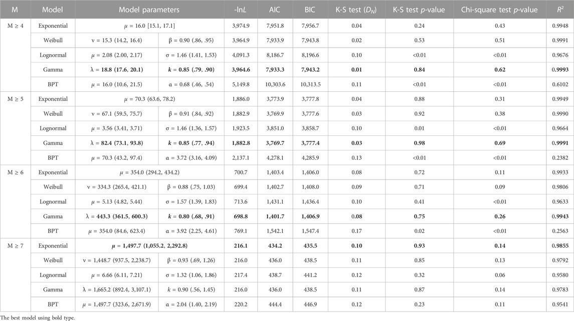
TABLE 3. Model parameters and AIC, BIC, K-S test, chi-square test and coefficient of determination results for earthquakes in Taiwan and adjacent areas (declustering by Gardner (1974) method).
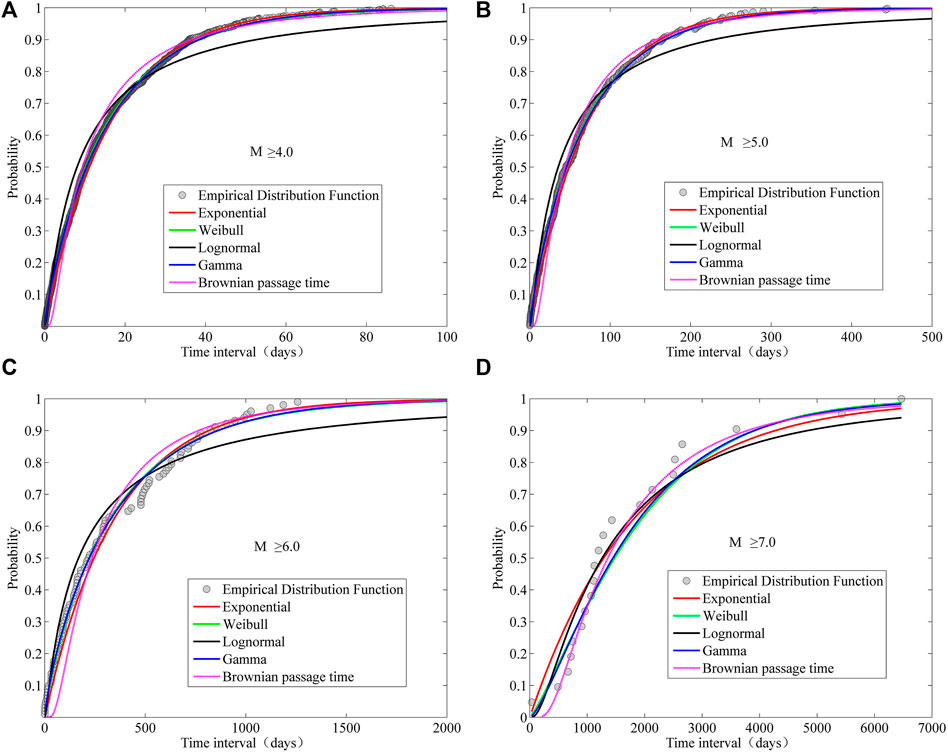
FIGURE 2. Cumulative probability distribution curves of time interval for five models for (A) M ≥ 4.0 earthquakes, (B) M ≥ 5.0 earthquakes, (C) M ≥ 6.0 earthquakes and (D) M ≥ 7.0 earthquakes.
This study also shows that for catalogs with any initial magnitudes, the K-S test does not reject its temporal distribution as exponential distribution in most circumstances, meaning that we can choose the statistical model able to yield the best description of temporal distribution of earthquakes by GOF measures, but we cannot reject that earthquake time series also follows other statistical models. This also means that in the current probabilistic seismic hazard analysis, it is reasonable to assume that the main shocks follow exponential distribution in time. However, when calculating occurrence rates, it would be more reasonable to adopt the optimal statistical model.
To ensure the robustness of the conclusions, the same analysis was conducted using earthquake catalogs with aftershocks eliminated based on Reasenberg (1985)’s method. The model parameters and goodness-of-fit test values are given in Table 4. As can be seen, the goodness-of-fit test values of each model in Table 4 are very similar to those in Table 3, and the same conclusions can be made, which suggests that the results obtained in this paper are robust. Tables 3, 4 provide the recurrence intervals and 95% confidence intervals of events of various magnitudes, which has important reference value for computing seismic hazard in the Taiwan area.
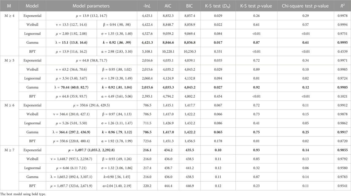
TABLE 4. Model parameters and AIC, BIC, K-S test, chi-square test and coefficient of determination results for earthquakes in Taiwan and adjacent areas (declustering by Reasenberg (1985)’s method).
3.2 Earthquake temporal correlation analysis
The temporal correlation of earthquakes is relative to the completely random distribution (exponential distribution) of events in time, which means that earthquakes occur in groups within a period of time and the occurrence of a large earthquake triggers more events. Earthquake temporal correlation has always been an issue of concern among seismologists, with important affect on earthquake prediction and seismic hazard analysis.
We used the DEA method to analyze the temporal correlation of earthquakes, with a scale parameter of d. When δ = .5, random variables conform to the Poisson distribution with no correlation between them. When δ > .5, the variables have correlation and long-term memory, that is, the occurrence of one event triggers the next. When the scale parameter is less than .5, there is negative interaction between earthquakes, that is, the occurrence of one earthquake delays the next event. In practice, when the sample size is small, the calculated scale value is less than .5 even if the time sequence follows the theoretical Poisson distribution (Tsai and Shieh, 2008).
As can be seen from Figure 3, a diagram of DEA results of earthquakes in Taiwan, the scale parameter δ for MW ≥ 4, MW ≥ 5, and MW ≥ 6 earthquakes is greater than .5 and the maximum can reach .61, indicating correlations between earthquakes above MW 4 in Taiwan. For MW ≥ 7 earthquakes, the scale parameter δ is .48, very close to .5, showing complete randomness and suggesting no correlation. In particular, the scale parameter δ of MW 4–6 earthquakes was calculated separately by removing the earthquakes of above MW 7.0 from the earthquake catalogs, and it was found that the scale parameter δ decreased significantly to about .53, slightly higher than .5, which means that the time correlation of earthquakes below magnitude 7 is relatively weak. The purpose of this analysis is to show that the strong time correlation of earthquake sequences above magnitude 4 is caused by the influence of large earthquakes (M7 + events) on moderate and strong earthquakes (M4 + events).
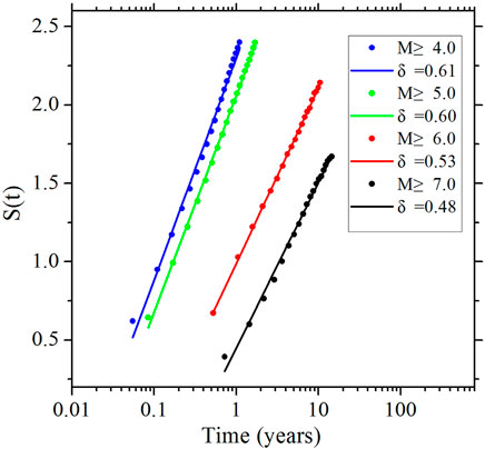
FIGURE 3. Variation of diffusion entropy of earthquakes with time and its scale value in Taiwan region. The dots in the figure represent entropy based on actual data, and the lines are the fitted Shannon entropy function based on time.
Then we used the kernel density estimation method of Geist and Parsons (2011) to smooth the earthquake catalogs with MW ≥ 4, MW ≥ 5, MW ≥ 6, and MW ≥ 7 events in the periods with complete catalogs on the time axis (Figure 4). In this paper, the smoothing kernel function is a Gaussian function, and the bandwidth is based on Silverman (1998)’s optimal bandwidth of
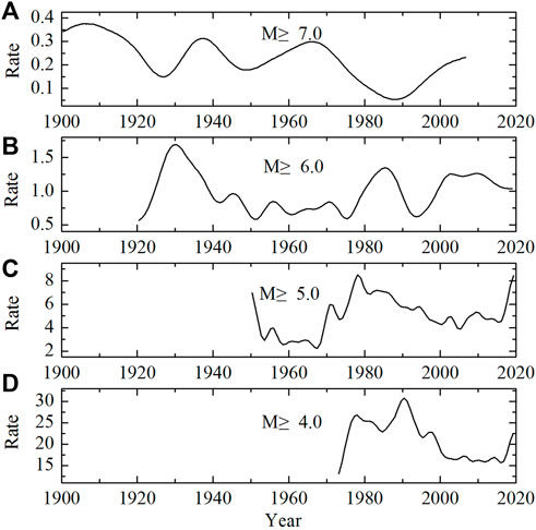
FIGURE 4. Kernel density estimation of earthquake sequences with different initial magnitudes on time axis. Subgraphs (A–D) in the figure are the time-varying curves of seismic rate with magnitudes M ≥ 7, M ≥ 6, M ≥ 5 and M ≥ 4, respectively.
After the active period of MW ≥ 7.0 earthquakes, the activity of earthquakes of or above MW 4–6 is obviously strengthened (Figure 4), which shows that the occurrence of MW ≥ 7 events can trigger subsequent moderate-strong earthquakes of or above MW 4–6, which is consistent with the aforementioned results of DEA analysis. As can be seen from Figures 4A, B, the trend of the rates shows that earthquakes of or above MW 7.0 were relatively active before 1920, and the frequency of seismicity above M6.0 increased obviously from 1920 to 1940. From 1960 to 1975, MW ≥ 7 events started to become active, and then seismicity of MW≥6 events began to increase, while MW ≥ 4 and MW ≥ 5 events were relatively active in the same period. The above analysis suggests that the occurrence of large earthquakes triggered subsequent moderate-strong earthquakes, which coincides with the accumulation of tectonic stress on the fault of large earthquakes. When tectonic stress accumulated to a certain extent, large earthquakes occurred again.
3.3 Occurrence probability of large earthquakes
As large earthquakes often cause serious casualties and damage to buildings, the probability of their future occurrence is an issue of great concern among scientists. We have already identified exponential distribution as the best model to describe the temporal distribution of MW ≥ 7.0 earthquakes, while Gamma, Weibull, lognorma, and Brownian passage time distributions also demonstrate good goodness-of-fit. To fully understand the occurrence probability of large earthquakes in Taiwan, we calculated the occurrence probability of future earthquakes of or above MW 7.0 based on the five distribution models.
Future probability may be calculated when the elapse time and recurrence intervals of large earthquakes and their uncertainties are known. Let Te (Escape time) be the time before the last earthquake occurred, then the conditional probability of at least one earthquake occurring in the future ΔT time is (Matthews et al., 2002):
where
According to the parameter values of each model calculated in Table 3, the occurrence probability of earthquakes of MW 7.0 or above in Taiwan in the next 1–50 years is calculated using Eq. 6 (Figure 5). The probability of occurrence calculated based on different models differs (Table 5), with the value calculated based on the exponential distribution model being the largest and that based on the Lognormal distribution the smallest. In the next 1 year, 5 years, 10 years, and 20 years, the maximum probability of MW ≥ 7.0 earthquakes in Taiwan is 21.6%, 70.4%, 91.3%, and 99.2%, respectively. Figure 5 shows the variation of the occurrence probability of MW ≥ 7.0 earthquakes in Taiwan with time calculated based on the five statistical distribution models. In the next 20 years, the probability of MW ≥ 7.0 earthquakes in Taiwan would reach almost 100% (Figure 5).
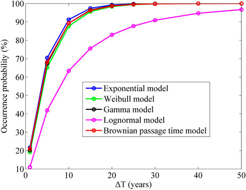
FIGURE 5. Variation of occurrence probability of M ≥ 7.0 earthquakes in Taiwan with time calculated based on five statistical distribution models.
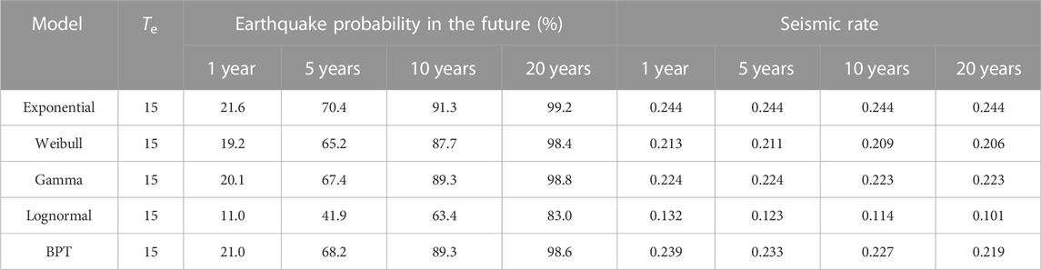
TABLE 5. Occurrence probability and seismic rate of M ≥ 7.0 earthquakes in Taiwan in the future.
While earthquake occurrence rate is used in probabilistic seismic hazard analysis, thus it is necessary to convert the probability of earthquake occurrence into effective occurrence rate. We used the formula
4 Conclusion and discussions
The present study provides a reliable and effective method for determining the optimal model of earthquake recurrence intervals. We adopt exponential, Gamma, Weibull, Lognormal, and Brownian passage time distributions as target models. Model parameters were regressed by the maximum likelihood method, and the goodness-of-fit was evaluated based on K-S test, AIC, and BIC values. The results show that Gamma distribution is the best model to describe the temporal distribution of MW 4-6 earthquakes in Taiwan, which is consistent with Chen et al. (2013)’s findings. For MW ≥ 7.0 earthquakes, exponential distribution yields the most accurate description of their distribution characteristics, which is consistent with the results of Shearer and Stark (2012) and Michael (2011) regarding the temporal distribution model of MW ≥ 7.0 earthquakes around the world. Through an analysis of the temporal distribution models, we found that events of or above MW 4–6 in Taiwan show time-dependence characteristics, suggesting that moderate-strong earthquakes are more susceptible to other earthquakes. Earthquakes of or above MW 7.0 show time independence. Sample size is an important factor affecting parameter estimation. In this study, only 26 events (M7+) were available, which may have some influence on the test results. Therefore, in this paper, we used multiple methods to analyze the time distribution of M7+ events, and all of them showed that they were time independent, ensuring the reliability of the conclusion.
To further validate the conclusions in the previous paragraph, we used the DEA method to study the correlation between earthquakes. The results show that MW 4–6 earthquakes in Taiwan are more susceptible to earthquakes of or above MW 7.0, and there is a time correlation between large and moderate-strong earthquakes. Furthermore, the kernel density estimation method was used to obtain the variation of seismicity frequency with time, with results showing that moderate-strong seismicity increased significantly after large events as well. This may be due to the long time of stress diffusion and adjustment following a large earthquake, which is manifested in the occurrence of a large number of moderate-strong earthquakes (Chéry et al., 2001; Shearer and Stark, 2012), and by long-term memory in statistical characteristics. Therefore, the influence of the latest strong earthquake on future moderate-strong earthquakes should be fully considered in the analysis of seismic hazards of a certain area. In previous studies, most scientists only paid attention to the temporal correlation between large earthquakes (Bufe and Perkins, 2005; Michael, 2011; Shearer and Stark, 2012; Daub et al., 2012; Kulkarni et al., 2013; Salditch, 2020), while our findings show that even after declustering, temporal correlation between large earthquakes and small and medium earthquakes still exists in the earthquake catalogs, which means that the occurrence of large earthquakes will trigger small and medium earthquakes, resulting in long-term memory in seismicity statistics.
We also calculated the occurrence probability of MW ≥ 7.0 earthquakes in Taiwan in the future based on the five models, and found that it may reach 70.4% and 91.3% in the next 5 and 10 years, respectively. In Chen et al. (2013)’s calculations, the probability of MW ≥ 7.0 earthquakes in Taiwan in the next 10 years is about 78.8%, which is lower than our result. This is due to the longer elapse time adopted in this study. In fact, the occurrence probability of MW ≥ 7.0 earthquakes calculated by Chen et al. (2013) in the next 20 years (94.9%) is equivalent of our results for the next 10 years (91.3%), showing relatively good consistency.
The findings in this study may provide reference for seismic hazard analysis and earthquake prediction in Taiwan.
Data availability statement
The original contributions presented in the study are included in the article/supplementary material, further inquiries can be directed to the corresponding author.
Author contributions
WX is responsible for the idea and writing of this manuscript. XL is responsible for data analysis. MG provides theoretical guidance for this manuscript.
Funding
This study was supported in part by the National Key Research and Development of China (Grant Numbers 2017YFC1500402), the Special Fund of Institute of Geophysics, China Earthquake Administration (Grant Number DQJB22Z03 and DQJB21Z07).
Acknowledgments
The authors thank the editor and reviewers for their valuable comments.
Conflict of interest
The authors declare that the research was conducted in the absence of any commercial or financial relationships that could be construed as a potential conflict of interest.
Publisher’s note
All claims expressed in this article are solely those of the authors and do not necessarily represent those of their affiliated organizations, or those of the publisher, the editors and the reviewers. Any product that may be evaluated in this article, or claim that may be made by its manufacturer, is not guaranteed or endorsed by the publisher.
References
Baiesi, M., and Paczuski, M. (2004). Scale-free networks of earthquakes and aftershocks. Phys. Rev. E 69 (6), 066106. doi:10.1103/physreve.69.066106
Bajaj, S., and Sharma, M. L. (2019). Modeling earthquake recurrence in the himalayan seismic belt using time-dependent stochastic models: Implications for future seismic hazards. Pure Appl. Geophys. 176, 5261–5278. doi:10.1007/s00024-019-02270-9
Beroza, G. C. (2012). How many great earthquakes should we expect? Proc. Natl. Acad. Sci. U. S. A. 109 (3), 651–652. doi:10.1073/pnas.1120744109
Bufe, C., and Perkins, D. (2005). Evidence for a global seismic-moment release sequence. Bull. Seismol. Soc. Am. 95 (3), 833–843. doi:10.1785/0120040110
Chen, C. H., Wang, J. P., Wu, Y. M., Chan, C. H., and Chang, C. H. (2013). A study of earthquake inter-occurrence times distribution models in Taiwan. Nat. Hazards 69, 1335–1350. doi:10.1007/s11069-012-0496-7
Chen, K.-P., and Chang, W.-Y. (2017). Estimating seismic hazards from the catalog of taiwan earthquakes from 1900 to 2014 in terms of maximum magnitude. Pure Appl. Geophys. 174, 1615–1627. doi:10.1007/s00024-017-1496-z
Chen, K.-P., and Tsai, Y.-B. (2008). A catalog of taiwan earthquakes (1900–2006) with homogenized mw magnitudes. Bull. Seismol. Soc. Am. 98 (1), 483–489. doi:10.1785/0120070136
Cheng, S. N., Wang, T. B., Lin, T. W., and Jiang, C. H. (2010). Establishment of Taiwan earthquake catalog. Seismol. Tech. Rep. Central Weather Bureau 54, 575–605.
Chéry, J., Merkel, S., and Bouissou, S. (2001). A physical basis for time clustering of large earthquakes. BSSA 91, 1685–1693.
Console, R., Murru, M., and Lombardi, A. M. (2003). Refining earthquake clustering models. J. Geophys. Res. 108 (B10), 2468. doi:10.1029/2002JB002130
Cornell, C. A. (1968). Engineering seismic risk analysis. Bull. Seismol. Soc. Am. 58, 1583–1606. doi:10.1785/bssa0580051583
Daub, E. G., Ben-Naim, E., Robert, G., and Johnson, P. A. (2012). Are megaquakes clustered? Geophys. Res. Lett. 39, L06308. doi:10.1029/2012GL051465
Fisher, R. A. (1922). On the mathematical foundations of theoretical statistics. Phil. Trans. Roy. Soc. Lond. 222, 309–368.
Gardner, J. K., and Knopoff, L. (1974). Is the sequence of earthquakes in southern California, with aftershocks removed, Poissonian? Bull. Seismol. Soc. Am. 64 (5), 1363–1367. doi:10.1785/bssa0640051363
Geist, E. L., and Parsons, T. (2011). Assessing historical rate changes in global tsunami occurrence. Geophys. J. Int. 187 (1), 497–509. doi:10.1111/j.1365-246x.2011.05160.x
Gibbons, J. D., and Chakraborti, S. (2003). Non-parametric statistical inference. 4th ed. Boca Raton, Fla: CRC Press, 645.
Hu, Y. X. (1990). Comprehensive probability method in seismic hazard analysis. Beijing: Seismological Press, 1–8.
Jiménez, A., Tiampo, K. F., Levin, S., and Posadas, A. M. (2006). Testing the persistence in earthquake catalogs: The Iberian Peninsula. Europhys. Lett. 73 (2), 171–177. doi:10.1209/epl/i2005-10383-8
Kulkarni, R., Wong, I., Zachariasen, J., Goldfinger, C., and Lawrence, M. (2013). Statistical analyses of great earthquake recurrence along the cascadia subduction zone. Bull. Seismol. Soc. Am. 103 (6), 3205–3221.
Lombardi, A. M., and Marzocchi, W. (2007). Evidence of clustering and nonstationarity in the time distribution of large worldwide earthquakes. J. Geophys. Res. 112, B02303. doi:10.1029/2006JB004568
Matthews, M. V., Ellsworth, W. L., and Reasenberg, P. A. (2002). A Brownian model for recurrent earthquakes. Bull. Seismol. Soc. Am. 92 (6), 2233–2250. doi:10.1785/0120010267
Mega, M. S., Paolo, A., Paolo, G., Latora, V., Palatella, L., Rapisarda, A., et al. (2003). Power-law time distribution of large earthquakes. Phys. Rev. Lett. 90 (18)–14. doi:10.1103/physrevlett.90.188501
Michael, A. J. (2011). Random variability explains apparent global clustering of large earthquakes. Geophys. Res. Lett. 38, L21301. doi:10.1029/2011gl049443
Nishenko, S. P., and Buland, R. (1987). A generic recurrence interval distribution for earthquake forecasting. Bull. Seismol. Soc. Am. 77 (4), 1382–1399.
Obi, E. O., Abong, A. A., and Ogbeche, J. U. (2017). Empirical study of the frequency and severity of earthquakes in taiwan. J. Geosciences Geomatics 5 (4), 167–172. doi:10.12691/jgg-5-4-1
Ogata, Y. (1998). Space-time point-process models for earthquake occurrences. Ann. Inst. Stat. Math. 50 (2), 379–402. doi:10.1023/a:1003403601725
Ogata, Y., and Zhuang, J. (2006). Space-time ETAS models and an improved extension. Tectonophysics 413 (1/2), 13–23. doi:10.1016/j.tecto.2005.10.016
Parsons, T., and Geist, E. L. (2012). Were global M≥8:3 earthquake time intervals random between 1900 and 2011? Bull. Seismol. Soc. Am. 102 (4), 1583–1592. doi:10.1785/0120110282
Pasari, S., and Dikshit, O. (2015). Distribution of earthquake interevent times in northeast India and adjoining regions. Pure Appl. Geophys. 172, 2533–2544. doi:10.1007/s00024-014-0776-0
Pasari, S., and Dikshit, O. (2018). Stochastic earthquake interevent time modeling from exponentiated Weibull distributions. Nat. Hazards 90, 823–842. doi:10.1007/s11069-017-3074-1
Petersen, M. D., Cao, T., Campbell, K. W., and Frankel, A. D. (2007). Time-independent and time-dependent seismic hazard assessment for the state of California: Uniform California earthquake rupture forecast model 1.0. Seismol. Res. Lett. 78 (1), 99–109. doi:10.1785/gssrl.78.1.99
Petersen, M. D., Moschetti, M. P., and Powers, P. M., (2014). Documentation for the 2014 update of the United States national seismic hazard maps. USGS Open-File Report, 2014–1091.
Reasenberg, P. (1985). Second-order moment of central California seismicity, 1969–1982. J. Geophys. Res. 90 (B7), 5479–5495. doi:10.1029/jb090ib07p05479
Salditch, L., Stein, S., Neely, J., Spencer, B. D., Brooks, E. M., Agnon, A., et al. (2020). Earthquake supercycles and long-term fault memory. Tectonophysics 774 (2020), 228289.
Scafetta, N., and West, B. J. (2004). Multiscaling comparative analysis of time series and a discussion on ‘earthquake conversations’ in California. Phys. Rev. Lett. 92, 138501–138504. doi:10.1103/physrevlett.92.138501
Schwartz, D. P., and Coppersmith, K. J. (1984). Fault behavior and characteristic earthquakes: Examples from the wasatch and san andreas fault zones. J. Geophys. Res. 89 (B7), 5681–5698. doi:10.1029/jb089ib07p05681
Shannon, C., and Weaver, W. (1948). A Mathematical theory of communication. Univ. of Illinois Press.
Sharma, M. L., and Kumar, R. (2010). Estimation and implementations of conditional probabilities of occurrence of moderate earthquakes in India. Indian J. Sci. Technol. 3 (7), 808–817.
Shearer, P. M., and Stark, P. B. (2012). Global risk of big earthquakes has not recently increased. Proc. Natl. Acad. Sci. U. S. A. 109 (3), 717–721. doi:10.1073/pnas.1118525109
Silverman, B. W. (1998). Density Estimation for Statistics and Data Analysis. 6th Edn. Boca Raton, FL: Chapman and Hall/CRC. 175.
Šipčić, N., Kohrangi, M., Papadopoulos, A. N., Marzocchi, W., and Bazzurro, P. (2022). The effect of seismic sequences in probabilistic seismic hazard analysis. Bull. Seismol. Soc. Am. XX, 1694–1709. doi:10.1785/0120210208
Taroni, M., and Akinci, A. (2021). Good practices in PSHA: Declustering, b-value estimation, foreshocks and aftershocks inclusion; a case study in Italy. Geophys. J. Int. 224, 1174–1187. doi:10.1093/gji/ggaa462
Tripathi, J. N. (2006). Probabilistic assessment of earthquake recurrence in the January 26, 2001 earthquake region of Gujrat, India. J. Seismol. 10, 119–130. doi:10.1007/s10950-005-9004-9
Tsai, C.-Y., and Shieh, C.-F. (2008). A study of the time distribution of inter-cluster earthquakes in Taiwan. Phys. A Stat. Mech. its Appl. 387, 5561–5566. doi:10.1016/j.physa.2008.05.023
Utsu, T. (1984). Estimation of parameters for recurrence models of earthquakes. Bull. Earthq. Res. Inst. Univ. Tokyo 59, 53–66.
Utsu, T. (2002). “Statistical features of seismicity,” in International handbook of earthquake & engineering seismology. Editors W. H. K. Lee, H. Kanamori, P. C. Jennings, and C. Kisslinger (Cambridge, Massachusetts, United States: Academic Press), 81A, 719–732.
Wang, Y. J., Chan, C. H., Lee, Y. T., Ma, K. F., Shyu, J. B. H., Rau, R. J., et al. (2016). Probabilistic seismic hazard assessment for Taiwan. Terr. Atmos. Ocean. Sci. 27 (3), 325–340. doi:10.3319/tao.2016.05.03.01(tem)
Werner, M. J., and Sornette, D. (2008). Magnitude uncertainties impact seismic rate estimates, forecasts, and predictability experiments. J. Geophys. Res. 113, B08302. doi:10.1029/2007JB005427
Yeh, Y. H., and Tsai, Y. B. (1981). Crustal structures of central Taiwan from inversion of P-wave arrival times. Bull. Inst. Earth Sci. 1, 83–102.
Zhou, Y., Aleksei, C., Sokolov, I. M., and Holger, K. (2016). A model of return intervals between earthquake events. EPL 114 (2016), 60003. doi:10.1209/0295-5075/114/60003
Zhuang, J., Chang, C.-P., Ogata, Y., and Chen, Y.-I. (2005). A study on the background and clustering seismicity in the Taiwan region by using point process models. J. Geophys. Res. 110, B05S18. doi:10.1029/2004JB003157
Keywords: statistical seismology, temporal distribution model, temporal correlation, gamma model, probability of earthquake occurrence
Citation: Xu W, Li X and Gao M (2023) Temporal distribution characteristics of earthquakes in Taiwan, China. Front. Earth Sci. 10:930468. doi: 10.3389/feart.2022.930468
Received: 28 April 2022; Accepted: 01 December 2022;
Published: 23 January 2023.
Edited by:
Iunio Iervolino, University of Naples Federico II, ItalyReviewed by:
Jawad Fayaz, Teesside University, United KingdomIlaria Spassiani, Istituto Nazionale di Geofisica e Vulcanologia (INGV), Italy
Copyright © 2023 Xu, Li and Gao. This is an open-access article distributed under the terms of the Creative Commons Attribution License (CC BY). The use, distribution or reproduction in other forums is permitted, provided the original author(s) and the copyright owner(s) are credited and that the original publication in this journal is cited, in accordance with accepted academic practice. No use, distribution or reproduction is permitted which does not comply with these terms.
*Correspondence: Weijin Xu, d2p4dXdpbkAxNjMuY29t