A Comparative Study of Six Hybrid Prediction Models for Uniaxial Compressive Strength of Rock Based on Swarm Intelligence Optimization Algorithms

Uniaxial compressive strength (UCS) is a significant parameter in mining engineering and rock engineering. The laboratory rock test is time-consuming and economically costly. Therefore, developing a reliable and accurate UCS prediction model through easily obtained rock parameters is a good way. In this paper, we set five input parameters and compare six hybrid models based on BP neural network and six swarm intelligence optimization algorithms–bird swarm algorithm (BSA), grey wolf optimization (GWO), whale optimization algorithm (WOA), seagull optimization algorithm (SOA), lion swarm optimization (LSO), firefly algorithm (FA) with the accuracy of two single models without optimization–BP neural network and random forest algorithm. Finally, the above eight models were evaluated and compared by root mean square error (RMSE), mean absolute percentage error (MAPE), coefficient of determination (R²), and a10 index to obtain the most suitable prediction model. It is indicated that the best prediction model is the FA-BP model, with a RMSE value of 4.883, a MAPE value of 0.063, and a R² of 0.985, and an a10 index of 0.967. Furthermore, the normalized mutual information sensitivity analysis shows that point load strength is the most effective parameters on the UCS, respectively.

Introduction

Uniaxial compressive strength is an important metric in rock mechanics and rock engineering, particularly in the evaluation of rock slope stability, tunneling design, and ore mining. On the other hand, the laboratory UCS test is time-consuming and costly. Many predict approaches have been offered to acquire the UCS quickly and cheaply.

The association between the physical and mechanical properties of rock samples and the UCS should be studied before the UCS can be predicted. Previous studies have found that a lot of rock parameters such as porosity, longitudinal wave velocity, point load strength, density, block impulse index (BPI), Young’s modulus, Schmidt hammer rebound number were correlated with UCS (Bieniawski, 1978; Barton et al., 1980; Nicholson and Bieniawski, 1990; Mitri et al., 1994; Hoke and Brown, 1997; Barton, 2002; Tsiambaos and Sabatakakis, 2004; Hao et al., 2018; Shan and Lai, 2018; He et al., 2019). After determining the parameters that are closely related to UCS, scholars usually use the empirical equation prediction method and machine learning methods to predict the UCS by these parameters.

When using the empirical equation to predict the UCS, scholars selected one or more parameters of rock samples and fit the statistical relationship between them and UCS. Part of scholars choose a single parameter and make predictions through different types of empirical equations. Leite and Ferland (2001) took the porosity as the input variable, carried out the linear fitting between the porosity and UCS, and found that the porosity and UCS were negatively correlated. Lashkaripour (2002) investigated the relationship between the porosity and the UCS by the exponential function, a similar conclusion was obtained with Leite and Ferland. Yasar and Erdogan (2004) conducted linear fitting on the longitudinal wave velocity and UCS. Yılmaz and Sendır (2002) fitted the Schmidt hammer rebound number and UCS with a function combining logarithmic function and linear function and obtained a reliable UCS prediction equation. Broch and Franklin (1972) corrected the size of rock samples to obtain the point load strength, established a linear function between the point load strength and UCS, and found that these two parameters are closely related. Ulusay and Gokceglu. (1998) developed a block impulse index test device, using the BPI as a parameter to indirectly evaluate UCS, and fitting it with a power function. Yagiz (2011) found that the slake durability index could be selected as an input variable for predicting UCS. Moreover, some scholars choose a variety of rock parameters to conduct this work. Sachpazis (1990) tested the UCS, Young’s modulus, and Schmidt hammer rebound number and established a regression equation between the three. Kayabasi et al. (2003) thought UCS was related to RQD value, Young’s modulus, and weathering degree of rock samples, and fit these three parameters and UCS, and the established a regression equation could meet the requirement. On the whole, the fitting equation proposed with the traditional statistical methods could meet the needs of projects.

With the development of advanced artificial intelligence methods, various non-linear UCS prediction models have been established. In these models, several physical and mechanical parameters of rock samples are usually chosen at the same time as the input variables. Through tensile strength, point load strength, and Young’s modulus, Armaghani et al. (2015) used the multiple regression analysis (MRA) and an adaptive neuro-fuzzy inference system (ANFIS) to obtain the UCS. Meulenkamp and Grima. (1999) used Young’s modulus, porosity, and density to predict UCS by the artificial neural network, and accurate prediction results were obtained. By using longitudinal BPI, Schmidt hammer rebound number, and wave velocity, point load index, Mishra and Basu et al. (2013) predicted the UCS with the farthest candidate selection model. The results indicated that Schmidt hammer rebound number and point load strength are excellent input variables. However, in the UCS prediction of shale, the longitudinal wave velocity is not a suitable input parameter. Rezaei et al. (2012) selected three parameters of density, Schmidt hammer rebound number, and porosity as the input variables, then the UCS was predicted by the fuzzy inference system (FIS). As a result, the predicted values were quite close to the laboratory-measured values. Furthermore, in this study, the sensitivity analysis showed that the Schmidt hammer rebound number was the best input variable among them. Mahmoodzadeh et al. (2021) chose long short term memory, deep neural networks, K-nearest neighbor, decision tree, and support vector regression to predict the UCS, and these models all got good prediction results. Even if these single prediction models could effectively predict the UCS, combined optimization algorithms are gradually being applied. Majdi and Beiki. (2010) established a genetic algorithm-optimized artificial neural network model to predict the UCS with density, RQD value, and porosity. The predicted results showed that better results could be obtained by the optimized model. Although the selected input variables are different, Mohamad et al. (2015) and Momeni et al. (2015) both employed the artificial neural network (ANN) combined with the particle swarm optimization (PSO) for the UCS prediction, the predicted results show that the optimized artificial neural network could give better-predicted values than before. On the basis of BPI, point load strength, Schmidt hammer rebound number, and longitudinal wave velocity, Xue and Wei (2020) compare the predicted results of least-squares support vector machine (LSSVM) optimized by genetic algorithm, ANFIS, FIS, and ANN. The optimized models’ accuracy is superior to the other three single models, according to the anticipated outcomes. Compared with the empirical equation prediction method, the prediction models established through different artificial intelligence algorithms have better performance in UCS prediction.

Although models built by artificial intelligence algorithms have found many applications in predicting UCS, its hybrid model building and the selection of input parameters still need to be refined. To find a suitable prediction algorithm and input parameters to predict UCS, in this paper, we selected five input parameters and used the six optimized BP neural networks with different swarm intelligence algorithms to predict the UCS, and evaluated the models through multiple evaluation indexes to find the optimal UCS prediction model. The findings of the study may be used as a reference to determine UCS quickly.

Basic Concepts and Algorithms of Predict Models

BP Neural Network

The input layer, middle layers, and output layer make up a BP neural network, with all neurons in the input and middle layers and the output layer linked. It is worth noting that neurons in the same layer are not linked. (Yan and Zeng, 2013). The topology of a BP neural network is shown in Figure 1. Through learning the input data, BP neural networks could establish a mapping relationship between input and output data, which leads to this method being used in multivariate non-linear system analysis.

FIGURE 1

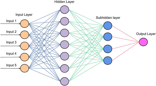
FIGURE 1. Schematic representation of the topology of a BP neural network.

Random Forest Algorithm

Leo Breiman (2001) invented the Random Forest (RF) method, which is a classic machine learning approach, which integrates multiple decision trees through integration learning (Bureau et al., 2010). Decision tree is a tree-like structure Figure 2 in which any internal node represents an attribute test. Each branch in decision tree represents an output result, and each leaf node represents a type. Within the integrated learning, multiple classifiers are generated, each classifier conducts learning and prediction without interfering and finally synthesizing a single prediction. The most widely used algorithms in integrated learning are the bagging algorithm and the boosting algorithm.

FIGURE 2

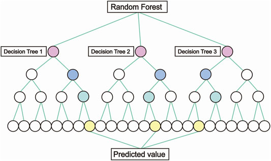
FIGURE 2. Schematic diagram of the random forest structure.

More explanations regarding the FA algorithm can be found in the literature (Yu et al., 2020a; Yu et al., 2020b; Yin et al., 2022).

Bird Swarm Algorithm

Bird is one of the flocking animals, and there are behaviors such as foraging, vigilance, and flight in their life (Meng et al., 2014). Bird swarm algorithm (BSA) is proposed inspired by these behaviors of birds. These community behaviors may be mimicked, and the swarm’s state of foraging, vigilance, and flight could be changed using precise rules. The analogous equation while the swarm is foraging is as follows:

$x_{i,j}^{t+1}=x_{i,j}^t+rand\left(\mathrm{0,1}\right)\times C\times \left(p_{i,j}-x_{i,j}^t\right)+rand\left(\mathrm{0,1}\right)\times S\times \left(g_j-x_{i,j}^t\right)(1)$

Where j is a positive integer between 1 and D, rand (0,1) is a uniformly distributed random number between 0 and 1, C is the cognitive acceleration factor, S is the social acceleration factor, and both C and S are positive integers, P_i,j is the previous optimal position of the i_th bird, and g_j represents the previous optimal position in the swarm.

When the swarm is alert, each bird tries to get closer to the swarm’s center. However, there is competition between every bird so that each bird does not move directly towards the swarm center. The flow chart of the BSA is shown in Figure 3. More explanations regarding the BSA algorithm can be found in the literature (Meng et al., 2015; Miramontes et al., 2018; Varol Altay and Alatas, 2019).

FIGURE 3

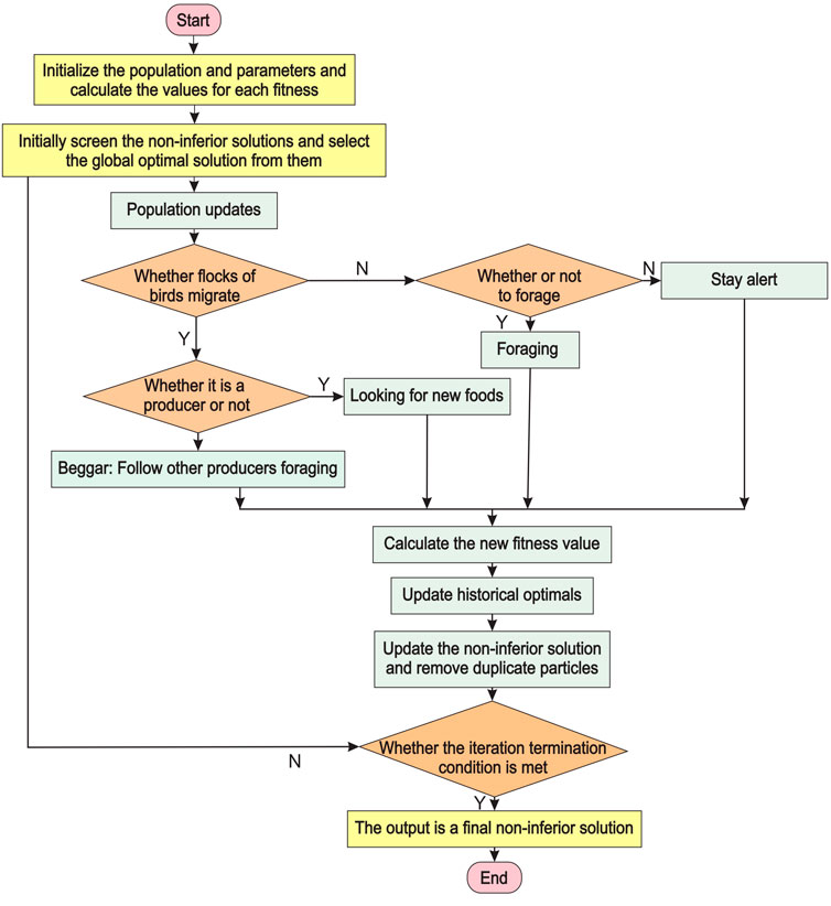
FIGURE 3. Flow chart of the bird swarm algorithm.

Grey Wolf Optimization

Grey wolf optimization (GWO) is a new meta-heuristic algorithm inspired by the grey wolf population’s social structure. (Mirjalili and Lewis. 2016). There are four different types of grey wolves, α, β, Δ, and ω, in the social hierarchy. The α wolf has the highest status, followed by the β wolf, then the Δ wolf, and the lowest rank is the ω wolf. Moreover, Hunting behavior is divided into three steps–locking for prey, surrounding the prey, and attacking the prey (Kishor and Singh, 2016).

In the beginning, the wolves approach the prey by stalking and chasing. Then a group of grey wolves will surround the prey until the prey stops moving. Finally, they attack the prey. The behaviors of a wolf population could be defined as:

${\overrightarrow{D}}_G=\left|{\overrightarrow{C}}_G.{\overrightarrow{X}}_{PG}\left(t_G\right)-{\overrightarrow{X}}_G\left(t_G\right)\right|(2)$

${\overrightarrow{X}}_G\left(t+1\right)={\overrightarrow{X}}_{PG}\left(t\right)-{\overrightarrow{A}}_G.{\overrightarrow{D}}_G(3)$

Where ${\overrightarrow{D}}_G$ is the distance between the wolf and the prey, ${\overrightarrow{X}}_{PG}$ is the prey position vector, ${\overrightarrow{X}}_G$ is the position vector of the grey wolf, t_G is the number of current iterations, ${\overrightarrow{A}}_G$ and ${\overrightarrow{D}}_G$ are the coefficient vectors. For a complete detail of the GWO algorithm, the readers can refer to the study conducted by Yu et al. (2019) and Yu et al. (2020c).

Whale Optimization Algorithm

Whales tend to hunt little fish at the surface of the ocean. Their feeding journey is a unique spiral upward path with many distinctive bubbles (Mirjalili and Lewis, 2016). There are three common behaviors in whales, searching for prey, surrounding prey, and hunting in the whale optimization algorithm (WOA).

Before hunting the prey, when ${\overrightarrow{A}}_W$ is greater than 1 or less than −1, the whale in the group randomly selects prey referring to each other’s positions so that the global search ability would be improved, this behavior could be written as:

${\overrightarrow{D}}_W=\left|{\overrightarrow{C}}_W.{\overrightarrow{X}}_{\text{rand}}\left(t_W\right)-{\overrightarrow{X}}_W\left(t_W\right)\right|(4)$

${\overrightarrow{X}}_W\left(t_W+1\right)={\overrightarrow{X}}_{\text{rand}}\left(t_W\right)-{\overrightarrow{A}}_W\cdot {\overrightarrow{D}}_W(5)$

Where ${\overrightarrow{X}}_{\text{rand}}$ is the randomly chosen location variable for the current whale population, ${\overrightarrow{D}}_W$ is the distance between the whale and the prey; ${\overrightarrow{X}}_W$ is the position vector of the optimal solution, t_W is the number of current iterations, ${\overrightarrow{A}}_W$ and ${\stackrel{\rightharpoonup }{C}}_W$ are both the coefficient vectors. For more details, equations and implementation process of the WOA can be referred tothe published studies in literature (Aljarah et al., 2016; Mirjalili and Lewis, 2016; Mafarja and Mirjalili, 2017).

Seagull Optimization Algorithm

Migrating and feeding are the most essential characteristics of seagulls, and the seagull optimization method is based on these activities. To avoid colliding, each bird is at a distinct place. Seagulls may fly towards the direction of the best landing spot. Seagull groups maneuver in a spiral manner when hunting for prey. (Dhiman and Kumar, 2019).

To avoid colliding with other seagulls as they migrate, the new position of the seagull might be determined using the additional variable A as follows:

$C_s\left(t_s\right)=A\times P_s\left(t_s\right)(6)$

Where C_s is a new position that is not in conflict with other seagulls, P_s is the seagull’s present location, t_s is the current iteration. A reflects the seagull’s movement behavior in the given search space, and it may be calculated as:

$A=f_{\text{c}}-\left[t_s\times \left(f_{\text{c}}/MA{X}_{\text{iteration}}\right)\right](7)$

Where f_c is the frequency of the control variable A, with a value linearly decreasing from 2 to 0. To have a better understanding regarding the SOA optimization technique, other studies in literature can be considered (Dhiman and Kumar, 2019; Dhiman et al., 2020; Panagant et al., 2020).

Lion Swarm Optimization

Lion swarm optimization is a new intelligence optimization algorithm proposed to simulate lion hunting. There are three types of lions in the population: lion king, lioness, and young lion. The update of their position follows different rules. The algorithm initializes the lion pride positions. Similar to other swarm intelligence optimization algorithms, the parameters in LSO need to be initialized before optimization starts (Yazdani and Jolai, 2016).

The lion king travels in a small area around the best prey during hunting, and the corresponding position update equation is:

$X_{\text{m}}^{t_L+1}=g^{t_L}\left(1+\gamma \left(p_{\text{m}}^{t_L}-g^{t_L}\right)\right)(8)$

Where X_m is the update position of the lion king, γ is a random number that fits a normal distribution between N (0,1); $g^{t_L}$ is the population optimal solution in the t_Lth iteration; and $p_{\text{m}}^{t_L}$ is the historical optimal solution for the m_th individual in the t_Lth iteration.

Through collaborative hunting, lionesses catch their prey, and this behavior can be described as:

$X_i^{t_L+1}=\frac{P_i^{t_L}+P_c^{t_L}}{2}\left(1+{\alpha }_f\gamma \right)(9)$

Where X is the position of the lioness moving, $P_c^{t_L}$ is the historical optimal solution for a randomly selected predation partner in the lioness’ pride during the ${\text{t}}_L$ iteration; ${\alpha }_{\text{f}}$ is the lioness’ range perturbation factor, which mainly affects the lioness’ range of movement so that the lioness can search for prey at a larger range and reduce the enclosure after finding prey. A complete version of the LSO optimization algorithm can be seen in previous work (Yazdani and Jolai, 2016).

Firefly Algorithm

Firefly algorithm (FA) is a group search-based stochastic optimization algorithm. There are a few parameters in FA. No complex operations such as variation and crossover, and the corresponding flow chart is shown in Figure 4.

FIGURE 4

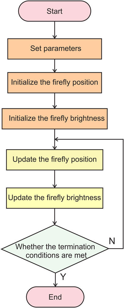
FIGURE 4. Flow chart of the firefly algorithm.

There are two pivotal parameters in this method–light intensity and attractiveness (Gandomi et al., 2011).

The light intensity function can be described as:

$I\left(r_{ij}\right)=I_0{\text{e}}^{-\gamma r_{ij}^2}(10)$

Where I₀ is the initial light intensity of the firefly, r is the distance between two fireflies, γ is defined as the light intensity absorption coefficient, which could describe light lost in the propagation.

If two fireflies i and j are located at ${\overrightarrow{X}}_{iF}$ and ${\overrightarrow{X}}_{jF}$, respectively, the distance between them can be calculated through Euclidean distance as:

$r_{ij}=\Vert {\overrightarrow{X}}_{iF}-{\overrightarrow{X}}_{jF}\Vert =\sqrt{{\displaystyle \sum _{k=1}^D{\left(X_{ik}-X_{jk}\right)}^2}}(11)$

Where D is the spatial dimension of the solution problem, X_ik is the coordinates of the i_th firefly in the k_th dimension.

The attractiveness of FA diminishes monotonically as the distance between them increases, and the attractiveness function β(r) could be defined as.

$\beta \left(r\right)={\beta }_0{e}^{-\gamma r^2}(12)$

Where β₀ is the attraction at the light source. A complete version of the FA optimization algorithm can be seen in previous works (Fister et al., 2013; Gandomi et al., 2013).

Database and Data Presentation

Selection of Input and Output Parameters

There are five input parameters–porosity, Schmidt hammer rebound number, longitudinal wave velocity, point load strength, Young’s modulus, and one output parameter–the UCS in this paper. The first four input parameters could be obtained through non-destructive testing methods (Stroffek and Lesso, 2001; Liu et al., 2020). Moreover, the point load strength is easy to obtain in the field test. These five parameters have been used more often in many previous similar prediction models and are trustworthy parameters.

Database

The experimental data from the literature (Tugrul and Zarif, 1999; Dincer et al., 2008; Dehghan et al., 2010; Armaghani et al., 2015) were collected to obtain the database in this paper, which includes a total of 158 test results, as shown in Table 1. Since the number of samples is too large, a matrix analysis plot is drawn to show the data (Figure 5), which examines the correlation between the input and output variables. It is indicated that there is a negative correlation between the porosity and the remaining four input variables. (The Corr in Figure 5 means Pearson correlation coefficient). Moreover, longitudinal wave velocity, Schmidt hammer rebound number, point load strength, and Young’s modulus are positively correlated with each other. To evaluate whether there are outliers in the data, a violin plot is drawn, as shown in Figure 6. The data we utilized in this study is evenly distributed. There are no obvious abnormal data in this database.

TABLE 1

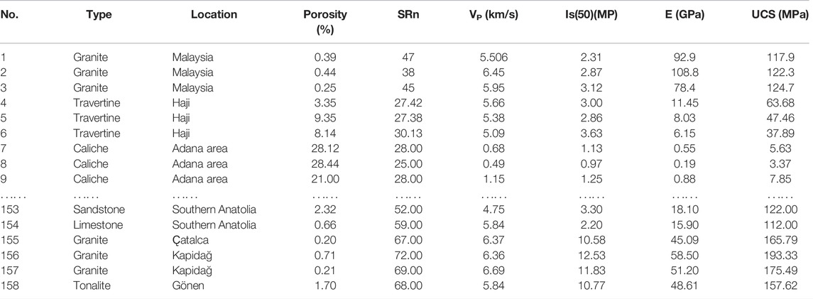
TABLE 1. Rock sample data.

FIGURE 5

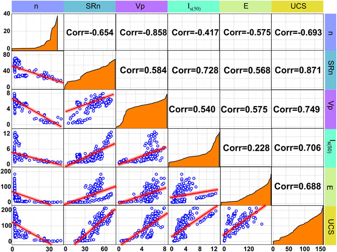
FIGURE 5. Data matrix.

FIGURE 6

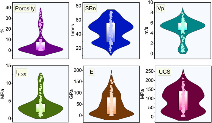
FIGURE 6. Data violin plot.

Result Analysis

Parameters Initialization

Setting a proper ratio between the training samples and test samples in the dataset is significant. According to the Pareto principle, the training group number and the test group number should account for about 80% and 20% of the total samples (Forman and Peniwati, 1998; Yu et al., 2021). On the basis of this rule, in this study, the training group was set at 128 groups, accounting for 81%, and the test group was set at 30 groups, accounting for 19%. The initial parameters of the proposed six hybrid optimization models–SOA-BP, GWO-BP, WOA-BP, BSA-BP, LSO-BP and FA-BP are shown in Table 2.

TABLE 2

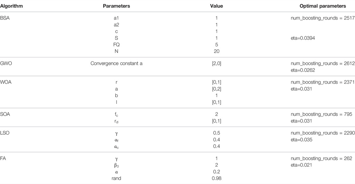
TABLE 2. Initial parameters for hybrid model optimization.

Predicted Results

After using the eight models to predict the UCS values, the actual values and the predicted values are shown in Figure 7. It is found that there are some big errors in the BP and RF models. The predicted values related to these six hybrid models are closer to the actual values.

FIGURE 7

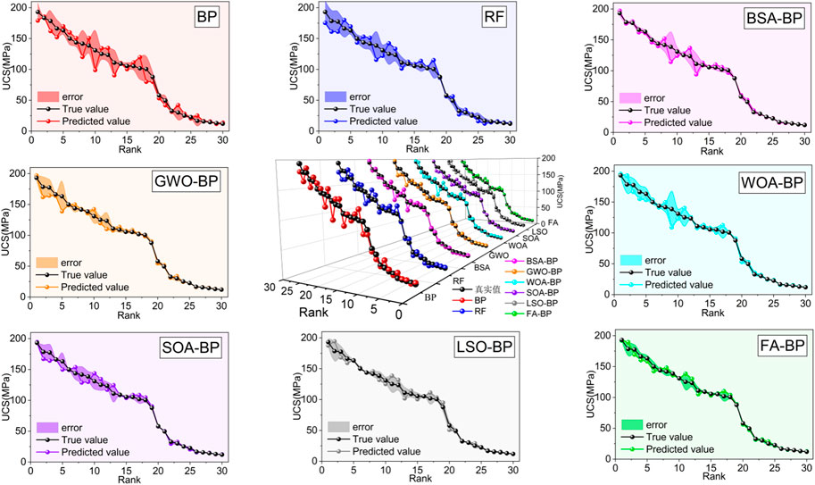
FIGURE 7. Predicted vs. true values.

Evaluation Method of Prediction Models

To evaluate the predicted results of the mentioned eight models, four parameters–RMSE, MAPE, R², a10 index were introduced. RMSE is a machine learning metric that measures the difference between the predicted and real values. The prediction model’s prediction effect improves as the RMSE decreases. (Barnston, 1992). RMSE could be calculated as:

$RMSE=\sqrt{{\displaystyle \sum _{i=1}^{N_0}{\left({\widehat{y}}_i-y_i\right)}^2}/N_0}(13)$

Where N₀ is the sample number in the test set, ${\widehat{y}}_i$ is the predicted result and y_i is the actual value.

MAPE calculates the difference between the expected and actual value. MAPE has a range greater than or equal to 0. Once the MAPE is close to 0, it is indicated that the corresponding model has little errors. When MAPE is greater than 1, the model is called as inferior model (Bollen et al., 2011). MAPE could be calculated as follows:

$MAPE=\frac{1}{N_0}{\displaystyle \sum _{i=1}^{N_0}\left|\frac{{\widehat{y}}_i-y_i}{y_i}\right|}\times 100(14)$

The coefficient of determination. When least squares are used for parameter estimation, R² is the ratio of explained sum of squares to sum of squares of deviations. And the larger the R² is, the more accurate the model is and the more significant the regression effect is. R² is a value between 0 and 1, where the closer it goes to 1, the better the model fits. It is generally considered that models with a R² over 0.8 are good. R² could be obtained as:

$R^2=1-\frac{{\displaystyle \sum _{i=1}^{N_0}\left(y_i-{\widehat{y}}_i\right)}}{{\displaystyle \sum _{i=1}^{N_0}\left(y_i-{\overline{y}}_i\right)}}(15)$

Where ${\overline{y}}_i$ is the mean of predicted values.

a10 index is a novel index in statistics. It is the ratio of the number of scatter points falling between ${\widehat{y}}_i=0.9y_i$ and ${\widehat{y}}_i=1.1y_i$ to the total number of samples in the test set. a10 lies between 0 and 1. If the a10 is close to 1, the corresponding model is better. a10 can be calculated by the following equation (Cevik et al., 2011):

$\text{a}10-\text{index}=\frac{m10}{M}(16)$

Where m10 is the number in test set falling between ${\widehat{y}}_i=0.9y_i$ and ${\widehat{y}}_i=1.1y_i$, M is the total number of samples in the test set.

Though the above four evaluate indexes, it is indicated that the FA-BP model is the best model in UCS prediction, with the RMSE of 4.883, a MAPE of 0.063, an R² of 0.985 and an a10 index of 0.967. The worst in the hybrid models was WOA-BP with the RMSE value of 8.130, the MAPE value of 0.102, the R² of 0.951, and the a10 index of 0.933. The other hybrid models all have an R² of 0.95 or higher, which shows that the hybrid models have better prediction results. On the contrary, the BP model had the RMSE value of 12.058, the MAPE value of 0.21, the R² of 0.941, and an a10 of 0.733. In the random forest, there are the RMSE value of 9.832, MAPE value of 0.153, R² of 0.945, and the a10 was 0.800. Their effects were all relatively poor. The relationship between the predicted and actual values was drawn in Figure 8. It could be seen in Figure 8 that all points are distributed on both sides of the perfect fit line. The data points corresponding to the FA-BP model are closest to the perfect fit line, and the data points are the most discrete in the BP model.

FIGURE 8

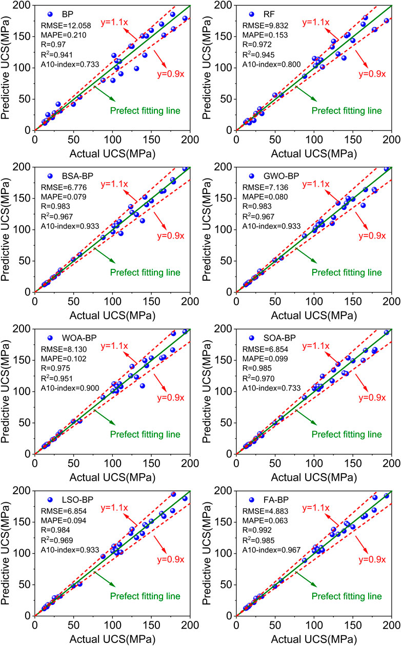
FIGURE 8. Correlation analysis between predicted and actual values.

To further evaluate the predict results of all prediction models, the Taylor diagrams were drawn to show the relevance of the standard deviation, root mean square error and correlation coefficient (Ciesielski et al., 2002), the relationship in these three parameters in Taylor diagrams could obtained by:

$R=\frac{\frac{1}{Z}{\displaystyle \sum _1^Z\left(l_n-\overline{l}\right)\left(m_n-\overline{m}\right)}}{{\sigma }_l{\sigma }_m}(17)$

Where R is the correlation coefficient, Z is the number of discrete points, l_n and m_n is discrete variables, σ₁ and σ_m is the standard deviation of l and m, $\overline{l}$ and $\overline{m}$ are the means of σ₁ and σ_m, respectively.

All Taylor diagrams are listed in Figure 9, and all the fitness value curves with the increasing iterations were collected, as shown in Figure 10. It could be seen from Figure 9 that the point corresponding to the FA-BP model is closest to the observation point in the 2D coordinates, indicating that this model has minimal prediction error. On the contrary, the point corresponding to the BP model is the furthest from the observation point, indicating that the prediction effect is poor. Moreover, the fitness curve corresponding to the FA-BP model decreases faster than that of other prediction models.

FIGURE 9

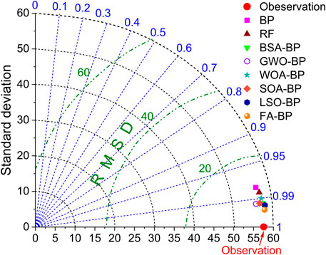
FIGURE 9. Taylor diagrams for all prediction models.

FIGURE 10

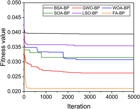
FIGURE 10. Variations of fitness value with the number of iterations.

Comprehensive Evaluation of UCS Prediction Models

To further analyze and compare the prediction performance and algorithm stability of these six hybrid models and two single models, we scored and evaluated the evaluation metrics for each model training set and testing set. Within the widely used grading method, all evaluation indexes need to be ordered, and then graded (Yin et al., 2021). However, two similar values may be classified into different levels in this method. To avoid this condition, we only calculate the scores for each model. The same evaluation index of each model is normalized by the following equation (Rao et al., 2008):

$y_i=\frac{x_i-{\min }_0}{{\max }_0-{\min }_0}(18)$

Where $y_i$ is the normalized value, $x_i$ is one of the evaluation indexes, min₀ and max₀ are the minimum and maximum values of each evaluation index, respectively.

After the normalization, all normalized values are in the range of 0–1. Noting that the larger R² value and a10 index value represent better models. On the contrary, if RMSE and MAPE are smaller, the corresponding model is better. When calculating the evaluation score of these four evaluation indexes, the evaluation scores for RMSE and MAPE are the difference between 1 and their corresponding normalized values. For the R² value and a10 index value, the evaluation score is equal to their normalized values. By replacing the traditional simple grading method with this standardized evaluation index, the problem of excessive disparity between the scores of close evaluation parameters can be solved (Chen et al., 2013).

All the obtained evaluation scores according to the calculation procedures were listed in Table 3 and Figure 11. As can be seen from Table 3, the scoring parameters of the training set and the testing set are relatively close in the same algorithm, which indicates that the algorithms are stable. Meanwhile, in order to better show the prediction effects of the eight algorithms, we accumulate the scores of the training and test sets of the algorithms to get the final scores of the algorithms, as shown in Figure 11. It is indicated from the evaluation results that the best prediction model is FA-BP, with a full score of 8. While the other five hybrid algorithms all scored between 5.123 and 6.196, the single model RF only scored 1.693 and the BP neural network scored 0.035. Noting that even if the other five hybrid models all have a worse effect than the FA-BP model, their predicted results are better than the unoptimized model–BP model and RF model.

TABLE 3

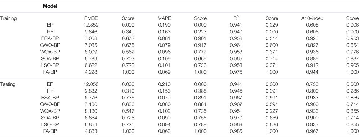
TABLE 3. List of evaluation parameters.

FIGURE 11

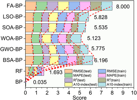
FIGURE 11. Multiple model score graph.

Sensitivity Analysis

It is evident from previous sections that the five input variables in this paper all have an obvious correlation with the UCS, but the significance level of each input variable is not yet known, and it needs to be further studied. Mutual information was often used by scholars in the information theory as a parameter to evaluate the correlation between two objects (Maes et al., 1997). Furthermore, normalized mutual information (NMI) can also be used to evaluate the relationships between each feature label. To make the overall predictive modeling scheme more convincing, the five input variables are evaluated by means of the Normalized Mutual Information (NMI) as a means of determining the importance of each variable parameter to the model. Mutual information I could be obtained as follows.

$I\left(X;Y\right)={\displaystyle \sum _x{\displaystyle \sum _{y}p\left(x,y\right)\log \frac{p\left(x,y\right)}{p\left(x\right)p\left(y\right)}}}(19)$

Where X and Y are two random variables, p(x,y) is the joint distribution of these two random variables, and p(x), p(y) is the marginal distribution of x and y. Mutual information I(X;Y) is the relative entropy of the joint distribution p(x,y) and the product distributions p(x)p(y). To compare the significance of all input variables, the mutual information should be normalized by the following equation:

$NMI\left(X;Y\right)=\frac{2I\left(X;Y\right)}{H\left(X\right)+H\left(Y\right)}(20)$

Where NMI(X;Y) is the normalized mutual information, and H(X) and H(Y) are the information entropy of the X and Y, respectively. On the basis of the values of the normalized mutual information, the significance levels of these input variables using in UCS prediction can be obtained, as shown in Figure 12. The sensitivity scores of the four quantities–Schmidt hammer rebound number, rock longitudinal wave velocity, point load test strength, and Young’s modulus are 0.777, 0.808, 0.828, and 0.833 respectively. Porosity has a low sensitivity score of 0.68. On the whole, the five parameters selected in this paper are in line with the requirements.

FIGURE 12

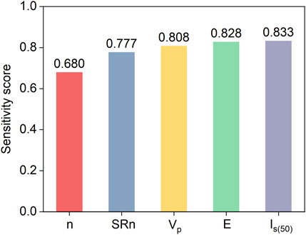
FIGURE 12. Input volume sensitivity analysis diagram.

Conclusion

In this paper, to predict the UCS of rock samples with the collected database with the artificial intelligence algorithm, six hybrid models–BSA-BP, GWO-BP, WOA-BP, SOA-BP, LSO-BP, FA-BP, and two classic models–BP and RF were developed. The predicted results obtained from the developed eight models were compared through four evaluation indexes and comprehensive scores. The following conclusions could be drawn:

(1) When predicting the UCS, six hybrid models based on the swarm intelligence optimization algorithms in this study are all significantly more accurate and significantly better than the BP neural network model and random forest model.

(2) The prediction accuracy of the used eight models from high to low is the FA-BP model, BSA-BP model, GWO-BP model, LSO-BP model, SOA-BP model, WOA-BP model, RF model, BP model. Among them, the FA-BP hybrid model showed the best comprehensive performance in six hybrid models and two single models. When carrying out the UCS prediction, the FA-BP model should be considered first.

(3) In the sensitivity analysis, porosity, Schmidt hammer rebound number, longitudinal wave velocity, point load strength, and Young’s modulus have the higher scores of 0.680, 0.777, 0.808, 0.828, and 0.833, respectively. They all could be utilized as input quantities when conducting the UCS prediction.

Data Availability Statement

The original contributions presented in the study are included in the article/Supplementary Material, further inquiries can be directed to the corresponding author.

Author Contributions

Investigation, YL and SZ; methodology, YL and SZ; writing-original draft preparation, YL and SZ; writing-review and editing, NJ and XL; supervision, XL; data curation, YL and SN; visualization, SN; funding acquisition, XL and NJ. All authors have read and agreed to the published version of the manuscript.

Funding

This project was supported by the National Natural Science Foundation of China (42072309, 41807265) and the Hubei Key Laboratory of Blasting Engineering Foundation (HKLBEF202002).

Conflict of Interest

The authors declare that the research was conducted in the absence of any commercial or financial relationships that could be construed as a potential conflict of interest.

Publisher’s Note

All claims expressed in this article are solely those of the authors and do not necessarily represent those of their affiliated organizations, or those of the publisher, the editors and the reviewers. Any product that may be evaluated in this article, or claim that may be made by its manufacturer, is not guaranteed or endorsed by the publisher.

References

Aljarah, I., Faris, H., and Mirjalili, S. (2016). Optimizing Connection Weights in Neural Networks Using the Whale Optimization Algorithm. Soft Comput. 22 (1), 1–15. doi:10.1007/s10462-019-09704-910.1007/s00500-016-2442-1

CrossRef Full Text | Google Scholar

Armaghani, D. J., Tonnizam Mohamad, E., Momeni, E., Monjezi, M., and Sundaram Narayanasamy, M. (2015). Prediction of the Strength and Elasticity Modulus of Granite through an Expert Artificial Neural Network. Arab. J. Geosci. 9 (1), 48. doi:10.1007/s12517-015-2057-3

CrossRef Full Text | Google Scholar

Barnston, A. G. (1992). Correspondence Among the Correlation, RMSE, and Heidke Forecast Verification Measures; Refinement of the Heidke Score. Wea. Forecast. 7 (4), 6992–7709. doi:10.1175/1520-0434(1992)007<0699:catcra>2.0.co;2

CrossRef Full Text | Google Scholar

Barton, N. R., Løset, F., Lien, R., and Lunde, J. (1980). Application of the Q-System in Design Decisions Concerning Dimensions and Appropriate Support for Underground Installations. In: Editor M. Bergmand, Subsurface space, New York: Pergamon, 2, 553–561. doi:10.1016/B978-1-4832-8421-7.50080-6

CrossRef Full Text | Google Scholar

Barton, N. (2002). Some New Q-Value Correlations to Assist in Site Characterisation and Tunnel Design. Int. J. Rock Mech. Min. Sci. 39 (2), 185–216. doi:10.1016/s1365-1609(02)00011-4

CrossRef Full Text | Google Scholar

Bieniawski, Z. T. (1978). Determining Rock Mass Deformability: Experience from Case Histories. Int. J. Rock Mech. Min. Sci. Geomechanics Abstr. 15 (5), 237–247. doi:10.1016/0148-9062(78)90956-7

CrossRef Full Text | Google Scholar

Bollen, J., Mao, H., and Zeng, X. (2011). Twitter Mood Predicts the Stock Market. J. Comput. Sci. 2 (1), 1–8. doi:10.1016/j.jocs.2010.12.007

CrossRef Full Text | Google Scholar

Breiman, L. (2001). Random Forests. Mach. Learn. 45, 5–32. doi:10.1023/a:1010933404324

CrossRef Full Text | Google Scholar

Broch, E., and Franklin, J. A. (1972). The Point-Load Strength Test. Int. J. Rock Mech. Min. Sci. Geomechanics Abstr. 9 (6), 669–676. doi:10.1016/0148-9062(72)90030-7

CrossRef Full Text | Google Scholar

Bureau, A., Dupuis, J. e., Falls, K., Lunetta, K. L., Hayward, B., Keith, T. P., et al. (2005). Identifying SNPs Predictive of Phenotype Using Random Forests. Genet. Epidemiol. 28 (2), 171–182. doi:10.1002/gepi.20041

PubMed Abstract | CrossRef Full Text | Google Scholar

Cevik, A., Sezer, E. A., Cabalar, A. F., and Gokceoglu, C. (2011). Modeling of the Uniaxial Compressive Strength of Some Clay-Bearing Rocks Using Neural Network. Appl. Soft Comput. 11 (2), 2587–2594. doi:10.1016/j.asoc.2010.10.008

CrossRef Full Text | Google Scholar

Chen, W., Yan, E. C., Cui, X. J., and Zhang, D. (2018). Variable Weight Interval Fuzzy Evaluation Method for Rock Mass Quality. Yangtze River. 49 (18), 72–74. doi:10.16232/j.cnki.1001-4179.2018.18.014

CrossRef Full Text | Google Scholar

Ciesielski, M. J., Kalla, P., Zheng, Z., and Rouzeyre, B. (2002). “Taylor Expansion Diagrams: A Compact, Canonical Representation with Applications to Symbolic Verification,” in Proceedings 2002 Design, Automation and Test in Europe Conference and Exhibition, Paris, France, 04-08 March 2002 (IEEE). doi:10.1109/DATE.2002.998286

CrossRef Full Text | Google Scholar

Dehghan, S., Sattari, G., Chehreh Chelgani, S., and Aliabadi, M. (2010). Prediction of Uniaxial Compressive Strength and Modulus of Elasticity for Travertine Samples Using Regression and Artificial Neural Networks. Min. Sci. Technol. (China) 20 (1), 41–46. doi:10.1016/s1674-5264(09)60158-7

CrossRef Full Text | Google Scholar

Dhiman, G., and Kumar, V. (2019). Seagull Optimization Algorithm: Theory and its Applications for Large-Scale Industrial Engineering Problems. Knowledge-Based Syst. 165, 169–196. doi:10.1016/j.knosys.2018.11.024

CrossRef Full Text | Google Scholar

Dhiman, G., Singh, K. K., Slowik, A., Chang, V., Yildiz, A. R., Kaur, A., et al. (2020). EMoSOA: a New Evolutionary Multi-Objective Seagull Optimization Algorithm for Global Optimization. Int. J. Mach. Learn. Cyber. 12 (2), 571–596. doi:10.1007/s13042-020-01189-1

CrossRef Full Text | Google Scholar

Dinçer, İ., Acar, A., and Ural, S. (2008). Estimation of Strength and Deformation Properties of Quaternary Caliche Deposits. Bull. Eng. Geol. Environ. 67 (3), 353–366. doi:10.1007/s10064-008-0146-1

CrossRef Full Text | Google Scholar

Emary, E., Zawbaa, H. M., and Hassanien, A. E. (2016). Binary Grey Wolf Optimization Approaches for Feature Selection. Neurocomputing 172, 371–381. doi:10.1016/j.neucom.2015.06.083

CrossRef Full Text | Google Scholar

Fister, I., Fister, I., Yang, X., and Brest, J. (2013). A Comprehensive Review of Firefly Algorithms. Swarm Evol. Comput. 13, 34–36. doi:10.1016/j.swevo.2013.06.001

CrossRef Full Text | Google Scholar

Forman, E., and Peniwati, K. (1998). Aggregating Individual Judgments and Priorities with the Analytic Hierarchy Process. Eur. J. Operational Res. 108 (1), 165–169. doi:10.1016/s0377-2217(97)00244-0

CrossRef Full Text | Google Scholar

Gandomi, A. H., Yang, X.-S., and Alavi, A. H. (2011). Mixed Variable Structural Optimization Using Firefly Algorithm. Comput. Struct. 89 (23-24), 2325–2336. doi:10.1016/j.compstruc.2011.08.002

CrossRef Full Text | Google Scholar

Gandomi, A. H., Yang, X.-S., Talatahari, S., and Alavi, A. H. (2013). Firefly Algorithm with Chaos. Commun. Nonlinear Sci. Numer. Simul. 18 (1), 89–98. doi:10.1016/j.cnsns.2012.06.009

CrossRef Full Text | Google Scholar

Hao, X., Du, W., Jiang, Y., Tannant, D., Zhao, Y., and Guo, Y. (2018). Influence of Bedding and Cleats on the Mechanical Properties of a Hard Coal. Arab. J. Geosci. 11 (9), 1-17. doi:10.1007/s12517-018-3541-3

CrossRef Full Text | Google Scholar

Hoek, E., and Brown, E. (1997). Practical Estimates of Rock Mass Strength. Int. J. Rock Mech. Mining Sci. 34 (8), 1165-1186. doi:10.1016/s1365-1609(97)80069-x

CrossRef Full Text | Google Scholar

He, M., Zhang, Z., Ren, J., Huan, J., Li, G., Chen, Y., et al. (2019). Deep Convolutional Neural Network for Fast Determination of the Rock Strength Parameters Using Drilling Data. Int. J. Rock Mech. Min. Sci. 123, 104084. doi:10.1016/j.ijrmms.2019.104084

CrossRef Full Text | Google Scholar

Kayabasi, A., Gokceoglu, C., and Ercanoglu, M. (2003). Estimating the Deformation Modulus of Rock Masses: a Comparative Study. Int. J. Rock Mech. Min. Sci. 40 (1), 55–63. doi:10.1016/s1365-1609(02)00112-0

CrossRef Full Text | Google Scholar

Lashkaripour, G. R. (2002). Predicting Mechanical Properties of Mudrock from Index Parameters. Bull. Eng. Geol. Environ. 61 (1), 73–77. doi:10.1007/s100640100116

CrossRef Full Text | Google Scholar

Leite, M., and Ferland, F. (2001). Determination of Unconfined Compressive Strength and Young's Modulus of Porous Materials by Indentation Tests. Eng. Geol. 59 (3-4), 267–280. doi:10.1016/s0013-7952(00)00081-8

CrossRef Full Text | Google Scholar

Liu, Z., Yan, D., and Niu, X. (2020). Insights into Pore Structure and Fractal Characteristics of the Lower Cambrian Niutitang Formation Shale on the Yangtze Platform, South China. J. Earth Sci. 31 (1), 169–180. doi:10.1007/s12583-020-1259-0

CrossRef Full Text | Google Scholar

Maes, F., Collignon, A., Vandermeulen, D., Marchal, G., and Suetens, P. (1997). Multimodality Image Registration by Maximization of Mutual Information. IEEE Trans. Med. Imaging 16 (2), 187–198. doi:10.1109/42.563664

PubMed Abstract | CrossRef Full Text | Google Scholar

Mafarja, M. M., and Mirjalili, S. (2017). Hybrid Whale Optimization Algorithm with Simulated Annealing for Feature Selection. Neurocomputing 260, 302–312. doi:10.1016/j.neucom.2017.04.053

CrossRef Full Text | Google Scholar

Mahmoodzadeh, A., Mohammadi, M., Hashim Ibrahim, H., Nariman Abdulhamid, S., Ghafoor Salim, S., Farid Hama Ali, H., et al. (2021). Artificial Intelligence Forecasting Models of Uniaxial Compressive Strength. Transp. Geotech. 27, 100499. doi:10.1016/j.trgeo.2020.100499

CrossRef Full Text | Google Scholar

Majdi, A., and Beiki, M. (2010). Evolving Neural Network Using a Genetic Algorithm for Predicting the Deformation Modulus of Rock Masses. Int. J. Rock Mech. Min. Sci. 47 (2), 246–253. doi:10.1016/j.ijrmms.2009.09.011

CrossRef Full Text | Google Scholar

Meng, X.-B. X., Gao, X. Z., Lu, L., Liu, Y., and Zhang, H. (2015). A New Bio-Inspired Optimisation Algorithm: Bird Swarm Algorithm. J. Exp. Theor. Artif. Intell. 28 (4), 673–687. doi:10.1080/0952813x.2015.1042530

CrossRef Full Text | Google Scholar

Meng, X., Yu, L., Gao, X., and Zhang, H. (2015). “A New Bio-Inspired Algorithm: Chicken Swarm Optimization,” in International Conference in Swarm Intelligence (Advances in Swarm Intelligence), 8794, 89–94. doi:10.1007/978-3-319-11857-4_10

CrossRef Full Text | Google Scholar

Meulenkamp, F., and Grima, M. A. (1999). Application of Neural Networks for the Prediction of the Unconfined Compressive Strength (UCS) from Equotip Hardness. Int. J. Rock Mech. Min. Sci. 36 (1), 29–39. doi:10.1016/s0148-9062(98)00173-9

CrossRef Full Text | Google Scholar

Miramontes, I., Guzman, J., Melin, P., and Prado-Arechiga, G. (2018). Optimal Design of Interval Type-2 Fuzzy Heart Rate Level Classification Systems Using the Bird Swarm Algorithm. Algorithms 11 (12), 206. doi:10.3390/a11120206

CrossRef Full Text | Google Scholar

Mirjalili, S., and Lewis, A. (2016). The Whale Optimization Algorithm. Adv. Eng. Softw. 95, 51–67. doi:10.1016/j.advengsoft.2016.01.008

CrossRef Full Text | Google Scholar

Mirjalili, S., Mirjalili, S. M., and Lewis, A. (2014). Grey Wolf Optimizer. Adv. Eng. Softw. 69, 46–61. doi:10.1016/j.advengsoft.2013.12.007

CrossRef Full Text | Google Scholar

Mishra, D. A., and Basu, A. (2013). Estimation of Uniaxial Compressive Strength of Rock Materials by Index Tests Using Regression Analysis and Fuzzy Inference System. Eng. Geol. 160, 54–68. doi:10.1016/j.enggeo.2013.04.004

CrossRef Full Text | Google Scholar

Mitri, H. S., Edrissi, R., and Henning, J. G. (1994). Finite Element Modelling of Cable-Bolted Stopes in Hard Rock Underground Mines. Presented at the SME Annual Meeting, New Mexico, Albuquerque, 94–116.

Google Scholar

Mohamad, E. T., Jahed Armaghani, D., Momeni, E., and Alavi Nezhad Khalil Abad, S. V. (2015). Prediction of the Unconfined Compressive Strength of Soft Rocks: a PSO-Based ANN Approach. Bull. Eng. Geol. Environ. 74 (3), 745–757. doi:10.1007/s10064-014-0638-0

CrossRef Full Text | Google Scholar

Momeni, E., Jahed Armaghani, D., Hajihassani, M., and Mohd Amin, M. F. (2015). Prediction of Uniaxial Compressive Strength of Rock Samples Using Hybrid Particle Swarm Optimization-Based Artificial Neural Networks. Measurement 60, 50–63. doi:10.1016/j.measurement.2014.09.075

CrossRef Full Text | Google Scholar

Nicholson, G. A., and Bieniawski, Z. T. (1990). A Nonlinear Deformation Modulus Based on Rock Mass Classification. Int. J. Min. Geol. Eng. 8 (3), 181–202. doi:10.1007/bf01554041

CrossRef Full Text | Google Scholar

Panagant, N., Pholdee, N., Bureerat, S., Kaen, K., Yıldız, A. R., and Sait, S. M. (2020). Seagull Optimization Algorithm for Solving Real-World Design Optimization Problems. Mater. Test. 62 (6), 640–644. doi:10.3139/120.111529

CrossRef Full Text | Google Scholar

Rao, Y., Lee, Y., Jarjoura, D., Ruppert, A., Liu, C., and Hsu, J. (2008). A Comparison of Normalization Techniques for MicroRNA Microarray Data. Stat. Appl. Genet. Mol. Biol. 7 (1). doi:10.2202/1544-6115.1287

PubMed Abstract | CrossRef Full Text | Google Scholar

Rezaei, M., Majdi, A., and Monjezi, M. (2012). An Intelligent Approach to Predict Unconfined Compressive Strength of Rock Surrounding Access Tunnels in Longwall Coal Mining. Neural Comput. Applic 24 (1), 233–241. doi:10.1007/s00521-012-1221-x

CrossRef Full Text | Google Scholar

Sachpazis, C. I. (1990). Correlating Schmidt Hardness with Compressive Strength and Young's Modulus of Carbonate Rocks. Bull. Int. Assoc. Eng. Geol. 42 (1), 75–83. doi:10.1007/bf02592622

CrossRef Full Text | Google Scholar

Shan, P. F., and Lai, X. P. (2018). Numerical Simulation of the Fluid-Solid Coupling Process during the Failure of a Fractured Coal-Rock Mass Based on the Regional Geostress. Transp. Porous Med. 124 (3), 1061–1079. doi:10.1007/s11242-018-1110-6

CrossRef Full Text | Google Scholar

Kishor, A., and Singh, P.K. (2016). Empirical Study of Grey Wolf Optimizer. In Proc. Fifth Int. Conf. Soft Computing for Problem Solving 436, 1037–49. doi:10.1007/978-981-10-0448-3-87

CrossRef Full Text | Google Scholar

Stroffek, E., and Lesso, I. (2001). Acoustic Method for Measurement of Young's Modulus of Steel Wire Ropes. Metalurgija 40 (4), 219–221.

Google Scholar

Tsiambaos, G., and Sabatakakis, N. (2004). Considerations on Strength of Intact Sedimentary Rocks. Eng. Geol. 72 (3-4), 261–273. doi:10.1016/j.enggeo.2003.10.001

CrossRef Full Text | Google Scholar

Tuğrul, A., and Zarif, I. (1999). Correlation of Mineralogical and Textural Characteristics with Engineering Properties of Selected Granitic Rocks from Turkey. Eng. Geol. 51 (4), 303–317. doi:10.1016/s0013-7952(98)00071-410.1016/s0013-7952(98)00071-4

CrossRef Full Text | Google Scholar

Ulusay, R., and Gokceglu, C. (1998). An Experimental Study on the Size Effect in Block Punch Index Test and its General Usefulness. Int. J. Rock Mech. Min. Sci. 35 (4-5), 628–629. doi:10.1016/s0148-9062(98)00024-2

CrossRef Full Text | Google Scholar

Varol Altay, E., and Alatas, B. (2019). Bird Swarm Algorithms with Chaotic Mapping. Artif. Intell. Rev. 53 (2), 1373–1414. doi:10.1007/s10462-019-09704-9

CrossRef Full Text | Google Scholar

Xue, X., and Wei, Y. (2020). A Hybrid Modelling Approach for Prediction of UCS of Rock Materials. Comptes Rendus. Mécanique 348 (3), 235–243. doi:10.5802/crmeca.17

CrossRef Full Text | Google Scholar

Yagiz, S. (2011). Correlation between Slake Durability and Rock Properties for Some Carbonate Rocks. Bull. Eng. Geol. Environ. 70 (3), 377–383. doi:10.1007/s10064-010-0317-8

CrossRef Full Text | Google Scholar

Yan, Z., and Zeng, L. (2013). “The BP Neural Network with MATLAB,” in 2013 International Conference on Electrical, Control and Automation Engineering (ECAE 2013), December 1-2, 2013 (Hong Kong: ECAE).

Google Scholar

Yaşar, E., and Erdoğan, Y. (2004). Estimation of Rock Physicomechanical Properties Using Hardness Methods. Eng. Geol. 71 (3-4), 281–288. doi:10.1016/s0013-7952(03)00141-8

CrossRef Full Text | Google Scholar

Yazdani, M., and Jolai, F. (2016). Lion Optimization Algorithm (LOA): A Nature-Inspired Metaheuristic Algorithm. J. Comput. Des. Eng. 3 (1), 24–36. doi:10.1016/j.jcde.2015.06.003

CrossRef Full Text | Google Scholar

Yılmaz, I., and Sendır, H. (2002). Correlation of Schmidt Hardness with Unconfined Compressive Strength and Young's Modulus in Gypsum from Sivas (Turkey). Eng. Geol. 66 (3-4), 211–219. doi:10.1016/s0013-7952(02)00041-8

CrossRef Full Text | Google Scholar

Yin, X., Liu, Q., Huang, X., and Pan, Y. (2022). Perception Model of Surrounding Rock Geological Conditions Based on TBM Operational Big Data and Combined Unsupervised-Supervised Learning. Tunn. Undergr. Space Technol. 120, 104285. doi:10.1016/J.TUST.2021.104285

CrossRef Full Text | Google Scholar

Yin, X., Liu, Q., Pan, Y., Huang, X., Wu, J., and Wang, X. (2021). Strength of Stacking Technique of Ensemble Learning in Rockburst Prediction with Imbalanced Data: Comparison of Eight Single and Ensemble Models. Nat. Resour. Res. 30 (2), 1795–1815. doi:10.1007/s11053-020-09787-0

CrossRef Full Text | Google Scholar

Yu, Z., Shi, X., Miao, X., Zhou, J., Khandelwal, M., Chen, X., et al. (2021). Intelligent Modeling of Blast-Induced Rock Movement Prediction Using Dimensional Analysis and Optimized Artificial Neural Network Technique. Int. J. Rock Mech. Min. Sci. 143, 104794. doi:10.1016/j.ijrmms.2021.104794

CrossRef Full Text | Google Scholar

Yu, Z., Shi, X., Qiu, X., Zhou, J., Chen, X., and Gou, Y. (2020b). Optimization of Postblast Ore Boundary Determination Using a Novel Sine Cosine Algorithm-Based Random Forest Technique and Monte Carlo Simulation. Eng. Optim. 53 (9), 1467–1482. doi:10.1080/0305215x.2020.1801668

CrossRef Full Text | Google Scholar

Yu, Z., Shi, X., Zhou, J., Chen, X., Miao, X., Teng, B., et al. (2019). Prediction of Blast-Induced Rock Movement during Bench Blasting: Use of Gray Wolf Optimizer and Support Vector Regression. Nat. Resour. Res. 29 (2), 843–865. doi:10.1007/s11053-019-09593-3

CrossRef Full Text | Google Scholar

Yu, Z., Shi, X., Zhou, J., Chen, X., and Qiu, X. (2020a). Effective Assessment of Blast-Induced Ground Vibration Using an Optimized Random Forest Model Based on a Harris Hawks Optimization Algorithm. Appl. Sci. 10 (4), 1403. doi:10.3390/app10041403

CrossRef Full Text | Google Scholar

Yu, Z., Shi, X., Zhou, J., Gou, Y., Huo, X., Zhang, J., et al. (2020c). A New Multikernel Relevance Vector Machine Based on the HPSOGWO Algorithm for Predicting and Controlling Blast-Induced Ground Vibration. Eng. Comput. 38 (2), 1905–1920. doi:10.1007/s00366-020-01136-2

CrossRef Full Text | Google Scholar