Temporal variations of the probability distribution of voronoi cells generated by earthquake epicenters

The area of the cells of Voronoi tessellations has been modelled through different probability distributions among which the most promising are the generalized gamma and tapered Pareto distributions. In particular the latter has been used to model times and distances between successive earthquakes besides area and perimeter of cells generated by earthquake epicenters. In the framework of nonextensive statistical mechanics applied in geophysics, variables like seismic moment, inter-event time or Euclidean distance between successive earthquakes or length of faults in a given region have been studied through the so-called q-exponential distributions obtained by maximizing the Tsallis entropy under suitable conditions. These distributions take also the name of generalized Pareto distributions in the context of the limit distributions of excesses. In this work we consider the spatial distribution of a set of earthquakes and its temporal variations by modelling the area of Voronoi cells generated by the epicenters through a generalized Pareto distribution. Following the Bayesian paradigm we analyze the recent seismicity of the central Italy and we compare the posterior marginal likelihood of the aforementioned distributions in shifting time windows. We point out that the best fitting distribution varies over time and the trend of all three distributions converges to that of the exponential distribution in the preparatory phase for the mainshock.

Introduction

Tessellations of space for a given set of points into non-overlapping cells play an important role in the study of spatial point patterns generated by natural and social phenomena. Among many possibilities of partitions, the Voronoi tessellation is probably the most popular; it has been applied in a wide variety of disciplines such as biology, astronomy, forestry, geology and ecology (Okabe et al. (2000)). Some of the statistical properties of spatial point patterns are related to the properties of the geometrical characteristics of the corresponding tessellation; in the case of the homogeneous Poisson point process the resulting Voronoi cells are called Poisson Voronoi (PV) cells. Even though the importance of this process has motivated many studies so far most of the results has not been obtained theoretically but through computer simulations; apart from the probability distribution of the cell length in $\mathbb{R}$, which is a Gamma (2,2) distribution, only a few moments of some characteristics of PV cells - such as the number of edges, the area, the perimeter - are known (Hinde and Miles (1980)), not their probability distributions. Fitting the histograms obtained by the simulation of some millions of PV cells Tanemura (2003) showed that the three-parameter (or generalized) gamma distribution fits quite well a wide range of probability densities of their geometrical characteristics in two- and three-dimensional spaces. With the aim to find a simpler functional form Ferenc and Neda (2007) obtained that the gamma distribution with parameters a = b = (3 d + 1)/2 gives an acceptable, even if less accurate, approximation of the size distribution of PV cells in d-dimensional spaces (d = 1, 2, 3). Zaninetti (2009) instead investigated non-Poissonian Voronoi diagrams associated with correlated seeds; he generated seeds in polar coordinates ρ and θ in the following way: the distance ρ from the center of the region is generated according to a probability distribution chosen between the product and the ratio of two Gamma (2,2), and the polar angle θ in degrees is given by θ = 360 Y with Y ∼ Unif (0, 1). Computer simulations provided evidence in favor of the conjecture according to which, in these cases, the area of the Voronoi cells follows the same distribution of the seeds.

In recent years some authors have begun to investigate how the properties of the cells change when boundaries are imposed to the study region. In particular Koufos and Dettmann (2019) considered PV cells located close to the boundaries of the quadrant ${\mathbb{R}}^{+}$ and obtained that the gamma distribution, with location-dependent parameters, provides a reasonably good approximation to the distribution of cell area. Gezer et al. (2021) compared the statistical properties of the area of PV cells in the infinite plane and of clipped cells in two bounded regions: the unit square and the convex hull of the points; they found that the generalized gamma distribution provides a good fit with parameters varying according to the location of the cell seed in the bounded region. It should be noted that, as the number of the points increases, the vast majority of cells are not affected by the imposition of boundaries; indeed Devroye et al. (2017) have shown that the asymptotic distribution of the Voronoi cell area is independent of the location of the seed and of the intensity measure underlying the Poisson point process.

In seismology Schoenberg et al. (2009) studied the point pattern of the earthquakes that occurred from 1984 to 2007 in Southern California through the Voronoi tessellation generated by their epicenters; they obtained that the tapered Pareto distribution, already used to describe the seismic moment (Jackson and Kagan (1999)), approximates the distribution of area and perimeter of the cells not intersecting with the boundary of the region better than the pure Pareto, log-normal and gamma distributions. This result can be explained by the spatial clustering of these events which implies many cells with a small area and some with a larger area than would be expected from a stationary point process. This behaviour is typical of heavy right-tailed distributions.

In the framework of the statistical physics a new distribution of the moment magnitude was derived from the q-exponential distribution (1 < q < 2) obtained by maximizing, under suitable constraints, a nonextensive generalization of the Boltzmann-Gibbs entropy given by the Tsallis entropy (Tsallis (2009); Vallianatos et al. (2015)). Following the example of Schoenberg et al. (2009) we have thought that the q-exponential distribution could describe, in addition to the earthquake size (Rotondi et al. (2022)), also the spatial properties of the seismic phenomenon such as the area of the Voronoi cells generated by the epicentral locations. This distribution also takes the name of generalized Pareto distribution in the context of the limit distributions of excesses (Bercher and Vignat (2008)); hence, hereafter, we use these two terms interchangeably.

The main aims of this work are: 1) to evaluate the fitting of the generalized Pareto distribution to the areas of Voronoi cells generated by the seismicity recorded in bounded regions of central Italy in recent years, b) to compare the performance of this distribution with that of the most promising probability distributions of the Voronoi cell area, that is, tapered Pareto and generalized gamma distributions, in time-varying windows with the same number of events. Parameter estimation is performed according to the Bayesian paradigm by applying Markov chain Monte Carlo (MCMC) methods, in particular the Metropolis-Hastings algorithm, to sample from the posterior probability distributions of the parameters (Roberts and Casella (2004)); hence the comparison is based on the ratio of the pairwise posterior marginal likelihoods of the abovementioned distributions. We will try to associate the probability distribution with the best performance to time periods characterized by a specific type of seismic activity; in particular we will notice that the likelihood of the three distributions generally assumes very different value from that of the exponential distribution apart from in a few time windows in the preparatory phase of the considered seismic crises in which the values of the four likelihoods are not significantly different.

Voronoi tessellation

Let us consider a finite number of n points P = {p_i ∈ S, i = 1, 2, … , n} distributed within some finite region $S\in {\mathbb{R}}^2$. The Voronoi tessellation partitions the region into a collection of disjoint subregions V = {V_i, i = 1, 2, … , n} called Voronoi cells, which have the following properties: V_i ∩ V_j = ∅ for i ≠ j, ${\cup }_{i=1}^n{V}_i=S$. Each cell V_i is defined as the set (polygon) of points of S which are closer to the corresponding seed p_i than any other point in P; hence:

$V_i=\left\{x\in S:\Vert x-p_i\Vert \le \Vert x-p_j\Vert \mathrm{f}\mathrm{o}\mathrm{r}j=\mathrm{1,2},\dots ,i-1,i+1,\dots ,n\right\}$

where ‖ ⋅‖ denotes Euclidean distance. If we join the points p_i and p_j associated with the cells V_i and V_j that share an edge, we obtain an undirected graph called a Delaunay triangulation of the convex hull of P. Figure 1 shows an example of Voronoi tessellation of n = 100 uniformly distributed points in the unit square. In this work we have constructed Voronoi tessellations using the deldir library (Turner (2018)) available within R (R Core Team (2018)).

FIGURE 1

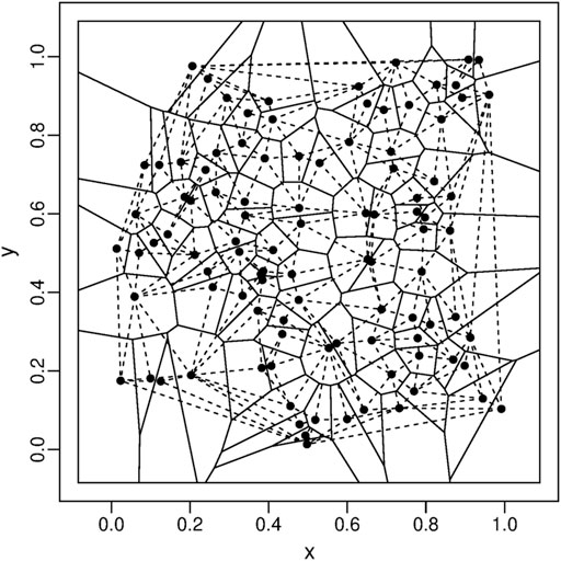
FIGURE 1. Voronoi tessellation of n =100 uniformly distributed points (black dots) bounded by the unit square and the convex hull of points; edges of the PV cells (solid lines) and Delaunay triangulation associated with the Voronoi diagram (dashed lines).

Probability distributions and Bayesian inference

We briefly present the three probability models adopted to describe the area of the Voronoi cells in a bounded region and we give the basic concepts on the Bayesian set-up we have followed in estimation and comparison of the three models. In general, let us assume that the data x = (x₁, x₂, … , x_n) are realizations of a random variable X whose density function belongs to the parametric family $\mathcal{F}=\{f(x;\theta ):\theta \in \mathrm{\Theta }\}$. In the Bayesian setting the parameter θ is considered as a random variable and we express our initial beliefs about it by specifying a distribution p₀(θ), termed prior distribution, which supplements the information provided by data and expressed by the likelihood $\mathcal{L}(f(\mathbf{x}|\theta ))={\prod }_{i=1}^{n}f(x_i;\theta )$. By applying the Bayes’ theorem we can combine the two sources of information into the posterior distribution:

$p\left(\theta |\mathbf{x}\right)=\frac{p_0\left(\theta \right)\mathcal{L}\left(f\left(\mathbf{x}|\theta \right)\right)}{{\int }_{\mathrm{\Theta }}{p}_0\left(\theta \right)\mathcal{L}\left(f\left(\mathbf{x}|\theta \right)\right)d\theta },(1)$

which enables us to get not only the parameter estimate, typically as the posterior mean E_p(θ), but also a measure of its accuracy by the posterior variance. These advantages however have a computational cost due to the evaluation of the integral, often high-dimensional, in (1); in fact when the prior distribution is not conjugate for the likelihood function, that integral does not have a closed-form expression and requires sophisticated numerical integration techniques. This difficulty has been tackled by the development of Markov chain Monte Carlo (MCMC) methods which produce simulated values from the posterior distribution (Roberts and Casella (2004)). In particular we apply the Metropolis-Hastings (MH) algorithm consisting of the following steps: a) generate an initial value θ₀ from p₀(θ) and set i = 0, b) draw a candidate $\tilde{\theta }$ from a proposal distribution q (θ∣θ_i), c) compute the acceptance probability

${\alpha }_i=\mathit{min}\left(1,\frac{\mathcal{L}\left(f\left(\mathbf{x}\mid \tilde{\theta }\right)\right)p_0\left(\tilde{\theta }\right)q\left({\theta }_i\mid \tilde{\theta }\right)}{\mathcal{L}\left(f\left(\mathbf{x}\mid {\theta }_i\right)\right)p_0\left({\theta }_i\right)q\left(\tilde{\theta }\mid {\theta }_i\right)}\right),$

and accept $\tilde{\theta }$ as θ_i+1 with probability α_i, or set θ_i+1 = θ_i with probability (1 − α_i). It can be shown that the generated sequence is a Markov chain having the posterior distribution (1) as equilibrium distribution. Since the first values of the chain are highly dependent on the starting value, we will use the sequence ${\left\{{\theta }_i\right\}}_{i=k+1}^{M+k}$, for large enough values of k and M, to estimate the posterior distribution p (θ∣x) and to approximate the posterior marginal log-likelihood:

$\log \mathcal{L}\left(f\left(\mathbf{x}\right)\right)={\int }_{\mathrm{\Theta }}\log \mathcal{L}\left(f\left(\mathbf{x}\mid \theta \right)\right)p\left(\theta \mid \mathbf{x}\right)d\theta \approx 1/M\sum _{j=k+1}^{M+k}\log \mathcal{L}\left(f\left(\mathbf{x}\mid {\theta }_j\right)\right)(2)$

that enables us to check how well the fitted model makes sense to explain the observed data. In general, given two statistical models f₁ (⋅|ϕ) and f₂ (⋅|η) we can compare them by $\mathrm{\Delta }=\log \mathcal{L}(f_1(\mathbf{x}))-\log \mathcal{L}(f_2(\mathbf{x}))$, and then, similar to the Bayes factor, we establish the degree of evidence in favor of the first model according to the value $\mathcal{K}$ of the Jeffreys scale (Kass and Raftery (1995); Gelman et al. (2004)). In the next Sections we introduce the three probability distributions we have chosen to model the Voronoi cell area and we give some elements on their Bayesian inference.

Q-Exponential - or generalized Pareto - distribution

The probability density function of the q-exponential distribution is given by:

$f_1\left(x\right)=\frac{1}{\beta }{\left(1-\frac{\left(1-q\right)}{\left(2-q\right)}\frac{x}{\beta }\right)}^{1/\left(1-q\right)}\text{for}x\ge 0\beta >0\text{and}1<q<2(3)$

where q is called the entropic index and β is the generalized expectation value, that is, the mean with respect to the escort probability distribution (Tsallis (2009)):

$f_q\left(x\right)=\frac{f^q\left(x\right)}{{\int }_0^{+\infty }{f}^q\left(x\right)dx}.(4)$

Since the q-exponential density function (3), for large x, goes to zero as a power x^−1/(q−1) it is a fat-tailed distribution; moreover, being always bounded below by the exponential density function and having

$\underset{x\to +\infty }{\lim }{e}^{tx}{\bar{F}}_1\left(x\right)=\underset{x\to +\infty }{\lim }{e}^{tx}{\left(1+\frac{q-1}{2-q}\frac{x}{\beta }\right)}^{-\left(2-q\right)/\left(q-1\right)}=+\infty \forall t>0(5)$

where ${\bar{F}}_1(x)=1-F_1(x)$, the q-exponential distribution is also heavy-tailed.

To improve the efficiency of the MH algorithm, we reparameterize the model (3) by setting θ = (2 − q)/(q − 1) with θ ∈ (0, + ∞). As prior distributions we adopt two lognormal distributions: θ ∼Lognormal (mean_θ, var_θ) and β ∼Lognormal (mean_β, var_β). We emphasize that here mean and var indicate the mean and variance of the random variable and not the mean and variance of its logarithm, as in the common representation of the lognormal distribution. We also choose lognormal distributions as proposal distributions; in particular, at the (i + 1)-th iteration, for θ we have $\text{Lognormal}({\theta }_i,{({\theta }_i/{\kappa }_1)}^2)$, and for β we have $\text{Lognormal}({\beta }_i,{({\beta }_i/{\kappa }_2)}^2))$, with θ_i and β_i as the current value of the respective Markov chain. The values of κ₁ and κ₂ are calibrated through pilot runs on the data so that the acceptance rate of the MH algorithm is about 25–40%.

Tapered Pareto distribution

The tapered Pareto distribution has cumulative distribution function

$F_2\left(x\right)=1-{\left(\frac{a}{x}\right)}^{\beta }\exp \left(-\frac{x-a}{\theta }\right)x\ge a(6)$

and density

$f_2\left(x\right)=\left(\frac{\beta }{x}+\frac{1}{\theta }\right){\left(\frac{a}{x}\right)}^{\beta }\exp \left(-\frac{x-a}{\theta }\right)x\ge a(7)$

where a > 0 is the minimum value of x, β is a shape parameter governing the power-law decrease in frequency as x increases, and θ is a parameter controlling the position of the exponential taper to zero in the frequency of large events (Vere-Jones et al. (2001)). It can be proved that the ${\int }_0^{+\infty }{e}^{tx}d{F}_2(x)$ is finite for 0 < t < 1/θ (Vaičiulis and Markovich (2021)); so the tapered Pareto distribution is light-tailed.

Similarly to the q-exponential distribution we adopt the lognormal distribution both as prior distribution and as proposal distribution of the three parameters with suitable values of κ₁, κ₂ and κ₃.

Generalized gamma distribution

The generalized gamma distribution, introduced by Stacy (1962), has the following three-parameter density function:

$f_3\left(x\right)=\frac{\beta }{\mathrm{\Gamma }\left(k\right)}\frac{x^{\beta k-1}}{{\alpha }^{\beta k}}\exp \left\{-{\left(x/\alpha \right)}^{\beta }\right\}\beta ,\alpha ,k>0(8)$

and it includes the exponential, Weibull and gamma distributions as special cases. In this form the generalized gamma distribution presented some difficulties in maximum likelihood estimate of the parameters; to overcome these problems Prentice (1974) proposed a different but equivalent form obtained through the transformation of variable $w=\sqrt{k}\left[\beta (\log x-\log \alpha )-\log k\right]$. In this way we obtain the generalized gamma density function:

$f_3\left(x\right)=\frac{\gamma {\left({\gamma }^{-2}\right)}^{{\gamma }^{-2}}}{\mathrm{\Gamma }\left({\gamma }^{-2}\right)}\exp \left\{\frac{\gamma \left(\frac{\log x-\mu }{\sigma }\right)-\exp \left\{\gamma \left(\frac{\log x-\mu }{\sigma }\right)\right\}}{{\gamma }^2}\right\}\frac{1}{\sigma x}(9)$

where μ = log  α + (log  k)/β ∈ (−∞, + ∞) is the location parameter, $\sigma =1/\left(\beta \sqrt{k}\right)\in (0,+\infty )$ is the scale parameter and $\gamma =1/\sqrt{k}\in (0,+\infty )$ is the shape parameter. This parameterisation is also adopted in the flexsurv and survival libraries available within R (R Core Team (2018)) and which we use to represent the generalized gamma distribution function in the figures reported in next Sections.

As prior distributions we adopt three lognormal distributions, while we choose the proposal distributions in the MH algorithm so that, at the (i + 1)-th iteration, $\tilde{\mu }$ is generated from $\text{Normal}({\mu }_i,{({\mu }_i/{\kappa }_1)}^2)$, $\tilde{\sigma }$ from $\text{Lognormal}({\sigma }_i,{({\sigma }_i/{\kappa }_2)}^2)$, and $\tilde{\gamma }$ from $\text{Lognormal}({\gamma }_i,{({\gamma }_i/{\kappa }_3)}^2)$.

Data

The data sequences analysed in this study are drawn from the Italian National Institute of Geophysics and Volcanology (Istituto Nazionale di Geofisica e Vulcanologia; INGV) web services: Italian Seismological Instrumental and Parametric Database (ISIDe) working group (2016), version 1.0, accessible at http://cnt.rm.ingv.it/en/iside (ISIDe Working Group (2007)). The parameters that define each earthquake of this catalog are the origin time, the hypocenter (i.e., geographic coordinates and depth) and the size that is expressed in different units of magnitude, as local magnitude M_L, duration magnitude M_D, and moment magnitude M_w. We have applied the orthogonal regression relationships: M_w = 1.066 M_L − 0.164 and M_w = 1.718 M_D − 1.897 (Gasperini et al. (2013)) to convert M_L and M_D to M_w so as to construct homogenous data sets. The coordinates of the epicenters are expressed in units of latitude and longitude in the WGS84 reference system; we have converted them to planar Universal Transverse Mercator (UTM) coordinate system (in km) through the Generic Mapping Tools (GMT) (Wessel and Smith (1998)) to be consistent with the Euclidean distance used by the deldir library in the construction of the Voronoi tessellations.

In recent decades central Italy was hit by strong seismic activity related to L’Aquila earthquake in 2009 and Amatrice-Norcia shocks in 2016. We analyze the seismicity recorded in the corresponding seismogenic areas in the years that preceded the mainshock and in part of the aftershock period to observe how the spatial distribution of the events changes. To do that we estimate the q-exponential, tapered Pareto, and generalized gamma distributions of the Voronoi cell area for time windows of a fixed number of events that shift at each new event. In the case of the exponential probability density: $f_4(x)=\lambda \exp \left\{-\lambda x\right\}$, we adopt the conjugate Gamma (0.01, 1) distribution as prior distribution of the λ parameter so that the expected area is about 100 km². For the three probability models under examination Table 1 reports the parameters of the prior distributions and the κ coefficients used in the proposal distributions of the MH algorithm to obtain suitable acceptance rates.

TABLE 1

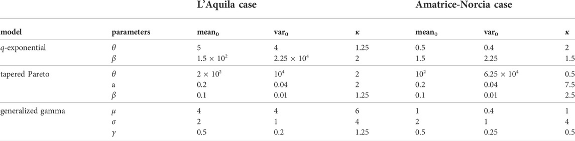
TABLE 1. Parameters of the prior distributions and κ coefficients used in the proposal distributions in MH algorithm.

L’Aquila case study

On 6 April 2009 (01:13:40 UTC, latitude 42.342, longitude 13.380), an M_w 6.1 earthquake struck central Italy, it was preceded by a M_w 4 shock on 30 March. The main event has been associated with the composite seismogenic source ITCS013 (Borbona-L’Aquila-Aremogna) of the Database of Individual Seismogenic Sources (DISS, version 3.2.1) (DISS Working Group (2018)), which is considered to have the potential for earthquakes of up to M_w 6.5. Considering the empirical relationships between magnitude and rupture length by Wells and Coppersmith (1992), the maximum expected rupture length in this area is about 18 km; moreover, since, according to Bowman et al. (1998), the seismic activation which precedes the major earthquakes should occur over a region with at most a characteristic length of about one order of magnitude larger than the maximum length, we consider a rectangular area centered on the epicenter, of latitude size (41.8, 43.0) degrees and longitude size (12.8, 13.8) degrees, which is included into the 33T zone of the UTM coordinate system. The events of M_w ≥ 2 recorded by ISIDe in this area during the temporal period from 7 April 2005 to the end of July 2009 are N = 2725. To analyze how the spatial distribution of the events varies and to investigate if these changes are linked to different phases of the seismic cycle we consider time windows of a fixed number - n = 100 - of events that shift at each new event. First, we fit the three probability distributions to the D^(k) dataset of each window, k = 1, 2, … , N − n + 1, and calculate their posterior marginal log-likelihood $\log \mathcal{L}(f_i({\mathbf{D}}^{(\mathbf{k})}))=1/m{\sum }_{j=1}^m\log f_i({\mathbf{D}}^{(\mathbf{k})}|{\mathrm{\Psi }}_i^{(j)}),i=\mathrm{1,2,3}$, with ${\left\{{\mathrm{\Psi }}_i^{(j)}\right\}}_{j=1}^m$ as the Markov chains of values of the parameter vectors Ψ₁ = (θ, β), Ψ₂ = (θ, a, β), and Ψ₃ = (μ, σ, γ), generated through the MH algorithm. Moreover we also compute the posterior marginal log-likelihood of the exponential distribution; all these values are associated with the time of the last event in the corresponding windows. Then, for each kth time window, we compute $i^{*}=\arg {\max }_{i=1,\dots ,4}\log \mathcal{L}(f_i({\mathbf{D}}^{(\mathbf{k})}))$, that is the $F_{i^{*}}$ probability distribution that provide the best performance among those under examination, and we evaluate the minimum discrepancy between the posterior marginal log-likelihoods of the best and of the other models given by ${\mathrm{\Delta }}_{i^{*}}^{(k)}=\log \mathcal{L}(f_{i^{*}}({\mathbf{D}}^{(\mathbf{k})})-{\max }_{j\ne i^{*},j=1,\dots ,4}\log \mathcal{L}(f_j({\mathbf{D}}^{(\mathbf{k})}))$. Comparing this discrepancy with the $\mathcal{K}$ values of the Jeffreys scale (Kass and Raftery (1995)) we establish the degree of evidence in favor of the $F_{i^{\ast }}$ model; in particular, set $\mathcal{K}={\log }_{e}10=2.3026$, ${\mathrm{\Delta }}_{i^{\ast }}^{(k)}\ge \mathcal{K}$ indicates strong strength of the evidence. Figure 2 shows the value of the posterior marginal log-likelihood of the best $F_{i^{\ast }}^{(k)}$ model for this level of evidence at each time window: red dots correspond to the q-exponential probability distribution (i^∗ = 1), blue dots to the tapered Pareto distribution (i^∗ = 2), and green dots to the generalized gamma distribution (i^∗ = 3). The legend in Figure 2 reports the percentages of time windows in which ${\mathrm{\Delta }}_{i^{\ast }}^{(k)}>\mathcal{K}$, that is the specific best model outperforms the others with strong evidence; this happens in about 78% of the intervals. The dots with slighter color indicate time windows in which $0<{\mathrm{\Delta }}_{i^{\ast }}^{(k)}<\mathcal{K}$, that is the evidence is less strong; in particular, from mid-September 2007 to January 2008 it is substantial $(1.1513<\mathcal{K}<2.3026)$, then it reduces and it is worth no more than a bare mention $(0<\mathcal{K}<1.1513)$ in favor of the exponential distribution (magenta dots) between December 2008 and January 2009, and finally it begins to increase until it returns strong in favor of the tapered Pareto distribution. In Figure 2 the red vertical lines indicate the time windows including the mainshock (solid line) and the M_w 4 30 March shock (dashed line) respectively. All this can be seen more clearly in Figure 3 which depicts magnification of the first 500 time windows of Figure 2 around the mainshock, precisely from April 2005 to 6 April 2009 (hr 8). The black dots represent the first quartile of the set of cell areas at each window. It can be noted that this quartile reaches the maximum in mid-February 2009, then it begins to decrease in correspondence to an increase of the number of small cells due to the concentration of the epicenters as the main phase approaches (De Santis et al. (2011)).

FIGURE 2

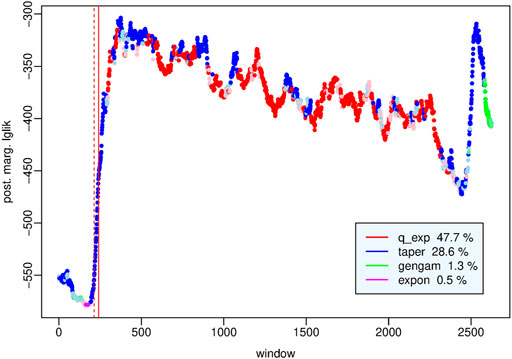
FIGURE 2. L’Aquila sequence - Posterior marginal log-likelihood of the probability distribution of Voronoi cell area that fits better than the other distributions to the dataset of each time window. The red vertical lines indicate the mainshock (solid line) and the M_w 4 30 March earthquake (dashed line) respectively.

FIGURE 3

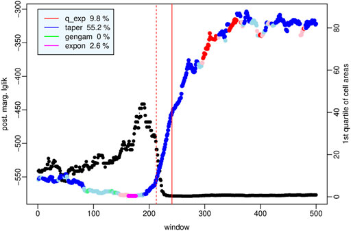
FIGURE 3. L’Aquila sequence - Magnification of Figure 2 in the period from April 2005 to 6 April 2009 (hr 8); the black dots indicate the first quartile of the set of cell areas in each time window.

Let us examine in detail the dataset for which each probability distribution performs best in order to understand which characteristics distinguish it from the others and in which phase of the seismic cycle it is more appropriate to use it. Statistical summaries of the four sets of Voronoi cell areas are in Table 2. The q-exponential distribution provides the best fit to the events associated with the $\widehat{k}$-th time window which covers few hours after the L’Aquila earthquake, that is $\widehat{k}=\arg {\max }_k{\mathrm{\Delta }}_{1^{\ast }}^{(k)}$; as expectable the cells of the Voronoi tessellation (top left-hand panel of Figure 4) are very small and concentrated around the epicenter of L’Aquila quake (red square) and along the rupture line, and the convex hull of the Delaunay triangulation (top right-hand panel) occupies only about 300 km². The bottom left histogram highlights the large number of very small area cells along with a few very large cells; the area varies in the range (0.151, 3336.13) (km²), median is 1.89 km², the sample mean is approximately 120 km² and the third quartile is less than 6 km². This behaviour is well modelled by a heavy-tailed density function such as the q-exponential as also shown by the Q-Q plot in the bottom right-hand panel. The legend reports the absolute difference between sampled and theoretical quantiles for each distribution; in this case, the minimum value is obtained by the q-exponential density function.

TABLE 2

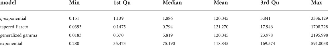
TABLE 2. Statistical summaries of the sets of Voronoi cell areas (in km²) to which each probability model fits best.

FIGURE 4

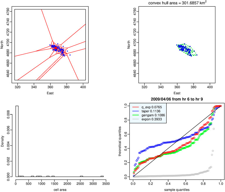
FIGURE 4. Dataset of the time window in which the q-exponential distribution provides the best fit. Top: Voronoi tessellation (left-hand panel) and Delaunay triangulation (right-hand panel). Bottom: histogram of the cell areas (left-hand panel) and Q-Q plot of the four probability distributions (right-hand panel). Red square indicates the epicenter of L’Aquila shock.

Figure 5 refers to the period from mid-June 2009 to early July 2009 in which the tapered Pareto distribution is the best model; the seismic activity is less concentrated, in fact the area of the Voronoi cells varies in narrower range (0.0393, 1708.73) (km²), the sample mean is still approximately 120 km² but the third quartile rises to 18 km². After about 3 months since the mainshock the secondary events begin to move away from its epicenter area so that the area of the convex hull is almost equal to 980 km². Also the Q-Q plot and the absolute difference between sampled and theoretical quantiles (bottom right-hand panel) show clear evidence in support of the tapered Pareto distribution as optimal model.

FIGURE 5

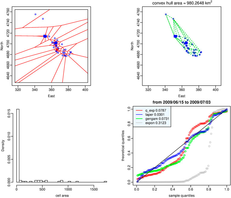
FIGURE 5. Dataset of the time window in which the tapered Pareto distribution provides the best fit. Top: Voronoi tessellation (left-hand panel) and Delaunay triangulation (right-hand panel). Bottom: histogram of the cell areas (left-hand panel) and Q-Q plot of the four probability distributions (right-hand panel). Red square indicates the epicenter of L’Aquila shock.

The dataset represented in Figure 6 consists of the events recorded from the end of June to mid-July 2009; the best fitting to the areas of the corresponding Voronoi tessellation is given by the generalized gamma distribution. The third quartile of the set of areas (−24 km²) is larger than that of the previous sets but there are still many very small cells probably due to the presence of localized clusters of secondary events. Also in this case the Q-Q plot and the absolute difference between sampled and theoretical quantiles support the generalized gamma distribution as optimal model in agreement with the posterior marginal log-likelihood.

FIGURE 6

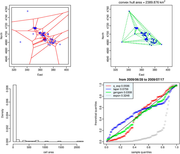
FIGURE 6. Dataset of the time window in which the generalized gamma distribution provides the best fit. Top: Voronoi tessellation (left-hand panel) and Delaunay triangulation (right-hand panel). Bottom: histogram of the cell areas (left-hand panel) and Q-Q plot of the four probability distributions (right-hand panel). Red square indicates the epicenter of L’Aquila shock.

A completely different situation is represented in Figure 7; the top left-hand panel shows the Voronoi tessellation generated by the rather scattered events that occurred in the period from mid-June 2007 to the end of January 2009. In Table 2 it can be seen that the range of variability of the cell areas is considerably reduced; while maintaining roughly the same mean, the first and third quartiles vary significantly. The four probability distributions behave similarly and fit well to the data but the posterior marginal likelihood of the exponential distribution is greater, although not substantially, than the likelihood of the other distributions.

FIGURE 7

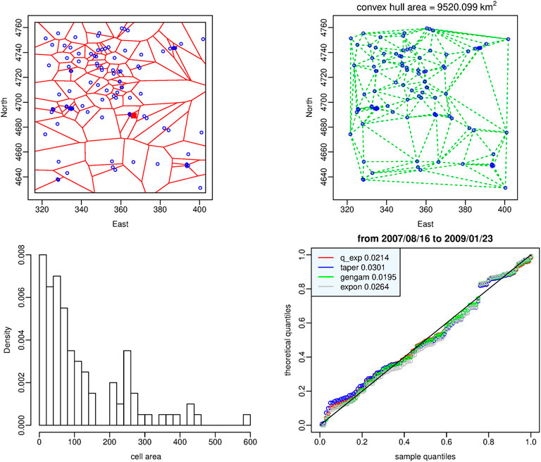
FIGURE 7. Dataset of the time window in which the exponential distribution provides the best fit. Top: Voronoi tessellation (left-hand panel) and Delaunay triangulation (right-hand panel). Bottom: histogram of the cell areas (left-hand panel) and Q-Q plot of the four probability distributions (right-hand panel). Red square indicates the epicenter of L’Aquila shock.

Observing Figures 2, 3 we can conclude that there is no single optimal probability distribution of the Voronoi cell area; the distribution that provides the best performance, as well as the spatial distribution of the events, varies over time according to the phases of the seismic cycle: (i) the exponential distribution exceeds the other distributions only in the period December 2008 - January 2009 which could mark the beginning of the preparatory phase, (ii) the q-exponential distribution characterizes mainly the initial, most active part of the aftershock sequence, (iii) the tapered Pareto distribution provides the best performance in the period encompassing the mainshock and covering the main phase up to approximately the time window in which all events are aftershocks, a few hours after the mainshock, (iv) the generalized gamma distribution characterizes, together with the tapered Pareto distribution, the quiescence period and the less active part of the aftershock sequence when seismicity begins to slowly diffuse at larger distances from the fault area.

Amatrice-Norcia case study

On 24 August 2016 (01:36:32 UTC, latitude 42.698, longitude 13.234), an M_w 6 earthquake hit central Italy with its epicenter between the village of Accumoli and the town of Amatrice. After a few years of relative quiescence that followed the aftershocks of the Aquila earthquake, the Amatrice shock marked the beginning of a more complex seismic crisis than the one that had just ended; in fact, what was first believed to be the mainshock, turned out to be later as a foreshock of the strongest quake (M_w 6.5) that would have occurred at the town of Norcia on 30 October 2016 (06:40:17 UTC, latitude 42.830, longitude 13.109). The seismic sequence lasted probably up to November 2018, and included several shocks among which there were three earthquakes with magnitudes greater than 5: on 24 August 2016, of M_w 5.3, and on 26 October 2016, of M_w 5.4 and M_w 5.9, and four earthquakes on 18 January 2017 of magnitude greater than 5: at 09:25 UTC M_w 5.1, at 10:14 UTC M_w 5.5, at 10:25 UTC M_w 5.4, and at 13:33 UTC M_w 5.0.

Since the Amatrice and Norcia earthquakes have been associated with the composite seismogenic source ITCS028 (Colfiorito-Campotosto) of the DISS (DISS Working Group (2018)), following the same criteria adopted to select the study region in the case of L’Aquila, we choose as study area a rectangular area of latitude size (42.3, 43.2) degrees and longitude size (12.7, 13.5) degrees centered around the Amatrice - Norcia earthquakes which also includes the L’Aquila epicenter and part of its aftershocks. To examine the spatial pattern of the events also in the period between the two seismic crises we extend the period under study back to the beginning of 2009 and up to June 2018. Moreover we raise the magnitude threshold to the value m₀ = 2.5 to reduce the effects of possible partial incompleteness of the catalogue in the first hours after the Norcia mainshock. In this way we obtain a data set of N = 5, 062 events drawn from ISIDe catalogue (ISIDe Working Group (2007)). Also in this case, we consider time windows of 100 events that shift at each new event. First we build the Voronoi tessellation generated by the events of each window, we fit the four probability models to each set of cell areas and then we compare the four probability distributions through pairwise differences of the respective posterior marginal log-likelihoods. Figure 8 shows, for each time window, the value of the posterior marginal log-likelihood of the model that behaves strongly better than the others; subdued colors indicate less evidence in favor of the optimal model; the vertical lines indicate the occurrence time of the Amatrice (dashed red), Norcia (solid red) and Capignano (M_w 5.5, 18 January 2018) (blue) earthquakes respectively. Figure 9 is a magnification of the same values around the Amatrice earthquake (red dashed line) from September 2010 to September 2016; black dots indicate the first quartile of the set of cell areas at each window. We note that the exponential distribution (magenta dots) outperforms the other distributions with less than substantial degree of evidence and not continuously in the period from late 2013 to February 2016, precisely up to 10 windows before the Amatrice shock; around the same time the first quartile of the sets of cell areas reaches its highest values.

FIGURE 8

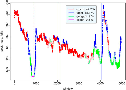
FIGURE 8. Amatrice-Norcia sequence - Posterior marginal log-likelihood of the probability distribution of Voronoi cell area that fits better than the other distributions to the dataset of each time window. The red vertical lines indicate the Amatrice (M_w 6.1) shock (dashed line) and the Norcia (M_w 6.5) mainshock (solid line) respectively; the blue vertical line indicates the Capignano (M_w 5.5) shock that occurred on 18 January 2017.

FIGURE 9

FIGURE 9. Amatrice-Norcia sequence - Magnification of Figure 8 in the period from mid-August 2009 to end of August 2016; the black dots indicate the first quartile of the set of cell areas in each time window. Red dashed vertical line indicates the Amatrice shock.

The legend of Figure 8 reports the percentages of time windows in which the specific best model outperforms the others with strong evidence. Recalling that our dataset contains two aftershock sequences, the large number of windows in which the q-exponential distribution is the optimal model supports the conclusion that this heavy-tailed distribution is suitable for describing the spatial pattern of highly clustered events; in particular it outperforms the other distributions in the following time intervals: from the L’Aquila (6 April 2009) shock up to September 2009, from a few hours after the Amatrice earthquake to early November 2016, and for half a month after the Capignano (M_w 5.5, 18 January 2017) shock. The tapered Pareto distribution instead characterizes the initial phase of the activation following the Amatrice and Capignano earthquakes until all the events in the time window are triggered events; moreover, the tapered Pareto distribution, together with the generalized gamma distribution, fit to the sets of cell areas in periods of low seismic activity such as that recorded from late October 2009 to mid-2013, and when the aftershocks begin to move away from the fault area as from December 2016 to the end of the period under study.

Final remarks

In this work we have a twofold objective: to propose a new probabilistic model - the q-exponential distribution - for the Voronoi cell area that is inspired by nonextensive statistical mechanics and to compare it with the most promising probability distributions in the literature to determine if there is a single optimal distribution according to the ratio of their posterior marginal likelihoods. We have therefore examined four distributions on the whole: the q-exponential, the tapered Pareto, the generalized gamma and the simple exponential distributions. Considering two seismic sequences recorded in central Italy in the last years and associated with the L’Aquila and Amatrice-Norcia destructive earthquakes we have verified that the probability distribution that best fits to the set of the areas of Voronoi cells generated by the epicenters of a fixed number of events included into shifting time windows varies over time apparently in correspondence with the phases of a seismic cycle (De Santis et al. (2011)).

The detailed examination of the results obtained for the four probability distributions in the two case studies allows us to discriminate different regimes:

• in a preparatory phase the exponential distribution exceeds weakly the other probability distributions in a few tens of time windows which cover some months before the foreshock activity; in this period we could also say that the four distributions are all basically suitable to describe a diffuse seismicity.

• Thereafter the activity tends to concentrate around the mainshock area with an increase in the variability range of the cell areas; this implies the best performance of the tapered Pareto distribution in what we can call the main phase. This phase comprises an event, which may not be the mainshock, but is strong enough to trigger a significant sequence of secondary events.

• The period of maximum concentration of the seismicity is characterized by the outperformance of the q-exponential distribution as it has heavier tail than the other distributions; we denote this period as primary clustering phase.

• The tapered Pareto and the generalized gamma distributions instead characterize the less active part of the aftershock sequence that we denote as secondary clustering phase, in which the concentration of events diffuses to a larger area surrounding the seismogenic area. A measure of this fact is given by the area of the convex hull in the Delaunay triangulation; in the top right-hand panel of Figures 4–7 we can note that this area is increasing as the best model moves from the q-exponential distribution to the tapered Pareto distribution, then to the generalized gamma distribution and finally to the exponential one.

• The spatial pattern of events in periods of quiescence is best modelled by the generalized gamma distribution but also by the tapered Pareto distrubtion.

It will, of course, be interesting to test the results obtained through further studies on different cases and in different seismotectonic settings.

Data availability statement

The datasets analyzed for this study can be found in the Italian Seismological Instrumental and Parametric Database (ISIDe) (ISIDe Working Group (2007)) at http://iside.rm.ingv.it.

Author contributions

All authors listed have made a substantial, direct, and intellectual contribution to the work and approved it for publication.

Funding

This research is partially funded by the INGV Project “Dynamic Planet” (CUP D53J19000170001), Topic 8-PANACEA 2021, supported by The Italian Ministry of Education, Universities and Research (MIUR).

Acknowledgments

The authors thank the Editor Prof. F. Vallianatos and the two reviewers.

Conflict of interest

The authors declare that the research was conducted in the absence of any commercial or financial relationships that could be construed as a potential conflict of interest.

Publisher’s note

All claims expressed in this article are solely those of the authors and do not necessarily represent those of their affiliated organizations, or those of the publisher, the editors and the reviewers. Any product that may be evaluated in this article, or claim that may be made by its manufacturer, is not guaranteed or endorsed by the publisher.

References

Bercher, J.-F., and Vignat, C. (2008). A new look at q-exponential distributions via excess statistics. Phys. A Stat. Mech. its Appl. 387, 5422–5432. doi:10.1016/j.physa.2008.05.038

CrossRef Full Text | Google Scholar

Bowman, D., Ouillon, G., Sammis, C., Sornette, A., and Sornette, D. (1998). An observational test of the critical earthquake concept. J. Geophys. Res. 103, 24359–24372. doi:10.1029/98jb00792

CrossRef Full Text | Google Scholar

De Santis, A., Cianchini, G., Favali, P., Beranzoli, L., and Boschi, E. (2011). The Gutenberg-Richter law and entropy of earthquakes: Two case studies in central Italy. Bull. Seismol. Soc. Am. 101, 1386–1395. doi:10.1785/0120090390

CrossRef Full Text | Google Scholar

Devroye, L., Györfi, L., Lugosi, G., and Walk, H. (2017). On the measure of Voronoi cells. J. Appl. Probab. 54, 394–408. doi:10.1017/jpr.2017.7

CrossRef Full Text | Google Scholar

DISS Working Group (2018). Database of individual seismogenic sources (DISS), version 3.2.1: A compilation of potential sources for earthquakes larger than M 5.5 in Italy and surrounding areas. Available at: http://diss.rm.ingv.it/diss/, Istituto di Geofisica e Vulcanologia. doi:10.6092/INGV.IT-DISS3.2.1

CrossRef Full Text | Google Scholar

Ferenc, J.-S., and Neda, Z. (2007). On the size distribution of Poisson Voronoi cells. Phys. A Stat. Mech. its Appl. 385, 518–526. doi:10.1016/j.physa.2007.07.063

CrossRef Full Text | Google Scholar

Gasperini, P., Lolli, B., and Vannucci, G. (2013). Empirical calibration of local magnitude data sets versus moment magnitude in Italy. Bull. Seismol. Soc. Am. 103, 2227–2246. doi:10.1785/0120120356

CrossRef Full Text | Google Scholar

Gelman, A., Carlin, J., Stern, H., and Rubin, D. (2004). Bayesian data analysis. New York: Chapman & Hall.

Google Scholar

Gezer, F., Aykroyd, R., and Barber, S. (2021). Statistical properties of Poisson-Voronoi tessellation cells in bounded regions. J. Stat. Comput. Simul. 91, 915–933. doi:10.1080/00949655.2020.1836184

CrossRef Full Text | Google Scholar

Hinde, A., and Miles, R. (1980). Monte Carlo estimates of the distributions of the random polygons of the Voronoi tessellation with respect to a Poisson process. J. Stat. Comput. Simul. 10, 205–223. doi:10.1080/00949658008810370

CrossRef Full Text | Google Scholar

ISIDe Working Group (2007). Italian Seismological Instrumental and Parametric Database (ISIDe), Istituto Nazionale di Geofisica e Vulcanologia (INGV).

Google Scholar

Jackson, D., and Kagan, Y. (1999). Testable earthquake forecasts for 1999. Seismol. Res. Lett. 70, 393–403. doi:10.1785/gssrl.70.4.393

CrossRef Full Text | Google Scholar

Kass, R., and Raftery, A. (1995). Bayes factors. J. Am. Stat. Assoc. 90, 773–795. doi:10.1080/01621459.1995.10476572

CrossRef Full Text | Google Scholar

Koufos, K., and Dettmann, C. (2019). Distribution of cell area in bounded Poisson Voronoi tessellations with application to secure local connectivity. J. Stat. Phys. 176, 1296–1315. doi:10.1007/s10955-019-02343-y

CrossRef Full Text | Google Scholar

Okabe, A., Boots, B., Sughara, K., and Chiu, S. (2000). Spatial tessellations concepts and applications of Voronoi diagrams. Chichester: John Wiley & Sons.

Google Scholar

Prentice, R. (1974). A log gamma model and its maximum likelihood estimation. Biometrika 61, 539–544. doi:10.1093/biomet/61.3.539

CrossRef Full Text | Google Scholar

R Core Team (2018). R: A language and environment for statistical computing. Vienna, Austria: R Foundation for Statistical Computing.

Google Scholar

Roberts, C., and Casella, G. (2004). Monte Carlo statistical methods. Springer.

Google Scholar

Rotondi, R., Bressan, G., and Varini, E. (2022). Analysis of temporal variations of seismicity through non-extensive statistical physics. Geophys. J. Int. 230, 1318–1337. doi:10.1093/gji/ggac118

CrossRef Full Text | Google Scholar

Schoenberg, F. P., Barr, C., and Seo, J. (2009). The distribution of Voronoi cells generated by Southern California earthquake epicenters. Environmetrics 20, 159–171. doi:10.1002/env.917

CrossRef Full Text | Google Scholar

Stacy, E. (1962). A generalization of the gamma distribution. Ann. Math. Stat. 33, 1187–1192. doi:10.1214/aoms/1177704481

CrossRef Full Text | Google Scholar

Tanemura, M. (2003). Statistical distributions of Poisson Voronoi cells in two and three dimensions. Forma 14, 221–247.

Google Scholar

Tsallis, C. (2009). Introduction to nonextensive statistical mechanics. Approaching a complex world. Springer. doi:10.1007/978-0-387-85359-8

CrossRef Full Text | Google Scholar

Turner, R. (2018). deldir: Delaunay triangulation and dirichlet (Voronoi) tessellation. R package version 0, 1–15.

Google Scholar

Vaičiulis, M., and Markovich, N. (2021). Estimating the parameters of a tapered Pareto distribution. Autom. Remote Control 82, 1358–1377. doi:10.1134/s000511792108004x

CrossRef Full Text | Google Scholar

Vallianatos, F., Michas, G., and Papadakis, G. (2015). “A description of seismicity based on non-extensive statistical physics: A review,” in chapter in the book earthquakes and their impact on society (Springer Natural Hazard, Springer).

CrossRef Full Text | Google Scholar

Vere-Jones, D., Robinson, R., and Yang, W. (2001). Remarks on the accelerated moment release model: Problems of model formulation, simulation and estimation. Geophys. J. Int. 144, 517–531. doi:10.1046/j.1365-246x.2001.01348.x

CrossRef Full Text | Google Scholar

Wells, D., and Coppersmith, K. (1992). New empirical relationships among magnitude, rupture length, rupture width, rupture area, and surface displacement. Bull. Seism. Soc. Am. 84, 974–1002.

Google Scholar

Wessel, P., and Smith, W. (1998). New, improved version of generic mapping Tools released. Eos Trans. AGU. 79, 579. doi:10.1029/98eo00426

CrossRef Full Text | Google Scholar

Zaninetti, L. (2009). Poissonian and non-Poissonian Voronoi diagrams with application to the aggregation of molecules. Phys. Lett. A 373, 3223–3229. doi:10.1016/j.physleta.2009.07.010

CrossRef Full Text | Google Scholar