 Xudong Jiang
 Junxing Cao*
- State Key Laboratory of Oil and Gas Reservoir Geology and Exploitation, Key Laboratory of Earth Exploration and Information Technology of Ministry of Education, Chengdu University of Technology, Chengdu, China
Seismic waves produce anomalies when they pass through hydrocarbons; these anomalies, which are commonly used to detect hydrocarbons, are manifested differently in different domains. Here, we propose a novel hydrocarbon detection method that combines Empirical Mode Decomposition (EMD), the Teager-Kaiser energy operator (TKEO), and the cepstrum. This method utilizes EMD’s ability to adaptively decompose signals, benefits from the TKEO’s superior performance regarding the focusing of instantaneous energy, and uses the sensitivity of cepstrum domain parameters to hydrocarbons. Here, applying the developed EMD-TKE-Cepstrum method to the Marmousi2 example revealed that it could describe the position and extent of hydrocarbons more clearly than the synchronous compression wavelet transform (SCWT) method. Applying the EMD-TKE-Cepstrum algorithm to field data further confirmed its potential regarding the identification of anomalies associated with hydrocarbon reservoirs.
Introduction
Hydrocarbon detection has always been the most critical step in reservoir prediction; it is the key condition that directly determines whether or not drilling is conducted at a given site. Seismic attenuation is an important indicator for the identification of gas-bearing hydrocarbons. The conventional method in gas-bearing prediction is to extract information on gas-sensitive seismic attributes from seismic data (Wang et al., 2020), for example, seismic attenuation attributes (Wang et al., 2016). Therefore, methods such as Fourier transform, wavelet transform, S transform, and synchronous compression wavelet transform (SCWT) are commonly used to conduct time-frequency analysis when locating gas in abnormal positions (Fawad et al., 2020). Furthermore, empirical mode decomposition (EMD) (Xue et al., 2014), variational mode decomposition (VMD) (Dragomiretskiy and Zosso (2014); Xue et al. (2018)), and other signal decomposition methods are often used to decompose the signal into different scale modes during gas detection. Data-driven deep learning gas prediction methods are also used, through attributes, to directly establish the relationship between gas and seismic data (Gao et al. (2020); Zhang and Alkhalifah (2020); Yang et al. (2021)). However, the ‘seismic attenuation’ method, which contains a physical meaning, has always been key to predicting the gas content. Thus, conducting conversion analysis for data with different frequencies is key to improving the prediction accuracy of this method for gas.
Since it was first proposed, the EMD method has occupied an important position in the field of time-frequency analysis (Chen and Fomel, 2018). EMD can adapt to time-frequency localization analysis, and can effectively extract the original information of a signal feature. This method decomposes the target signal based on the time scale characteristics of the data themselves, without the need for any basis function to be set in advance. Compared with Fourier decomposition and wavelet decomposition methods, which are based on a priori harmonic basis functions and wavelet basis functions, EDM has essential differences and advantages. EMD is used to decompose the bearing signal, and can diagnose faults (Li and He, 2012), decompose seismic signals, and then process a certain component to identify gas-bearing carbonate rocks (Hu et al., 2008). When combined with the Hilbert transform, EMD can determine the gas bearing nature of hydrocarbons from the energy distributions of different frequencies (Xue et al., 2013). The Teager–Kaiser energy operator (TKEO), meanwhile, is a nonlinear operator that can quickly focus signal energy density (Boudraa and Salzenstein, 2018). It is widely used in the field of oil and gas exploration. The TKEO directly locates a reservoir’s strong amplitude and high frequency energy, and then identifies the energy of the seismic facies (de Matos et al., 2009). The TKE calculation of the signal is processed by VMD to improve the instantaneous energy focus and realize high resolution oil and gas identification (Liu et al., 2017). The TKEO is used to optimize the pre-stack gather, which directly improves the sensitivity of the data to the gas content (Jiang X. et al., 2020). Combining EMD with the TKEO can also identify the location of gas-bearing characteristics; good results have been achieved using this approach (Xue et al., 2014), demonstrating the advantages and potential of combining the EMD and TKE operators. The cepstrum operator is a new operator that is derived from convolution signals; it is widely used in speech processing, geophysics, and medical field, among other fields (Tian and Cao (2012); Zayrit et al. (2020); Patil et al. (2022)). Its advantage lies in its signal unwinding ability; it can process signal homomorphism. Volcanic seismic signals have been converted to the cepstrum domain to achieve better data classification and feature recognition (Tong et al., 2016); by converting a thin layer signal to the cepstrum domain, the difference of said signal can be improved, allowing for thin reservoirs to be classified (Xie et al., 2016). The cepstrum, when combined with the wavelet transform, can effectively improve the geophysical response positioning of specific frequency bands, thus characterizing the gas content of a given target (Xue et al., 2016). These methods lay the foundation for using the cepstrum method to realize signal domain changes, while providing more information.
Inspired by the seismic attenuation through gas, and by the abovementioned recently developed methods, here we proposea novel hydrocarbon detection method based on the effective combination of EMD, TKEO, and the cepstrum. This method was developed with the aim of utilizing the adaptive decomposition capability of the EMD operator, the ability of the TKEO to focus the instantaneous energy, and the ability of the cepstrum to detect the spectral coefficient as a gas identification parameter, thereby allowing favorable gas-bearing zones to be delineated by the differences between high and low frequency cepstrum parameters. The effectiveness of the developed EMD-TKEO-Cepstrum method regarding reservoir characterization was then tested using Marmousi2 and field examples.
Theory
The difference between high- and low-frequency seismic data is often the key factor in gas detection. Most gas detection methods will use a specific high frequency, such as 50Hz, and a specific low frequency, such as 20Hz, to find the differences in oil and gas data at different frequencies. With the increase in exploration difficulty and the decrease in data signal-to-noise ratio, the gas-bearing characteristics become more and more insignificant. This paper proposes the EMD-TKE-Cepstrum method for the diversity of frequency changes. EMD algorithm is mainly used for adaptive frequency division of seismic data to obtain high-frequency and low-frequency components. The TKEO is mainly used to improve the instantaneous characteristics of data; the Cepstrum operator is used to divide the wavelet and the reflection coefficient, and the change rate is used to calibrate the variation characteristics of gas content in high and low-frequency data.
Empirical mode decomposition
Empirical Mode Decomposition (EMD) is suitable for nonlinear, non-stationary signals such as seismic signals; it can obtain intrinsic mode functions at different frequency component scales (Chen and Fomel, 2018). Considering a single channel seismic signal, defined as x(t), the main algorithms are as follows:
1) Find the extreme point. The maximum and minimum points of the seismic data are obtained by structural morphology algorithm (Jiang X.-d. et al., 2020).
2) Fit the envelope curve. The envelope u(t), v(t) of the signal is formed by cubic-spline interpolating the maximum and minimum points.
3) Mean envelope. The envelope mean is calculated as the first modal component,
4) Intermediate signal. Subtracting the mean envelope from the original signal to obtain the intermediate signal:
5) Determine the intrinsic mode function (IMF). IMF needs to meet two conditions: a) In the whole data segment, the number of extreme points and the number of zero crossings must be equal or the difference cannot exceed one. b) At any time, the average value of the upper envelope formed by the local maximum point and the lower envelope formed by the local minimum point is zero, that is, the upper and lower envelopes are locally symmetric with respect to the time axis.
The conventional EMD algorithm can generate the intrinsic mode values of different scales through the cycle of 1)-5); the frequency component is determined from high to low (Chen and Fomel, 2018). After EMD decomposition, the signal is arranged according to the frequency. Usually, the first component is the small-scale high-frequency component, and the subsequent component is the relatively low-frequency component. This paper aims to adaptively decompose the signal into relative high-frequency and relative low-frequency, so only one decomposition is carried out. The first component is the high-frequency component, and the remaining amount is the relative low-frequency component. This approach provided a basis for subsequent calculations based on the frequency domain.
Teager kaiser energy operator
The instantaneous feature is also one of the effective means for oil and gas detection. Because the seismic wavelet has a certain length and the influence across the geological body is continuous, the resolution of seismic data can be improved by enhancing the instantaneity of seismic data. The TKEO is a nonlinear filter that can effectively extract instantaneous features and improve signal recognition in scenarios that are affected by noise. It has good applicability in many fields. The TKEO, which is denoted as Ψc when operating on the x(t) signal, is given by:
where
where x(n) = x (nΔt) with Δt = 1/fs and
It can be seen from this algorithm that the biggest advantage of the TKEO is its instantaneity, because each point only needs three samples to calculate the energy. This efficient and simple algorithm can thus effectively capture the signal of instantaneous energy changes. The TKEO calculation of the high and low-frequency components separated by the EMD operator can enhance the temporality of the data to a certain extent and improve the resolution of the data.
Cepstrum coefficient
The cepstrum is widely used in speech signal processing for speech signal separation and localization (Patil et al., 2022). Its main function is to linearly separate two or more separate signals after convolution. In this regard, seismic data can be considered to represent the convolution of seismic wavelets and reflection coefficients. Therefore, here seismic signals were transformed from the time-frequency domain to the cepstrum domain, and the cepstrum coefficient was used to identify fluid.
Traditionally, the cepstrum of a time-series signal, x(t), can be obtained with the following equation:
where FFT represents the Fourier transform and IFT represents the inverse Fourier transform. The cepstrum can be understood as a logarithmic compression of autocorrelation sequences because it carries information similar to autocorrelation sequences.
The cepstral coefficient solution method was developed based on this method. For a seismic signal, x(n), 0, < ,n ≤ M (M stands for the length of the seismic signal. ) first divides said signal into frames. Supposing that the frame length is N, and that the step size k = 1, this method can be calculated as follows:
where F (•) stands for the framing processing. Usually, the signal is flipped at both ends and extended to a length of N/2, according to the step length, before processing. This is done to ensure the timeliness of the signal. At the same time, in order to reduce the marginal effect of framing on each signal, we usually use the Hamming window of the corresponding length to multiply and retain the key information of the signal. The cepstrum calculation can then be performed as follows:
where C(Q) represents the result of the cepstrum of the frame data and C(Q) = q1, q2, q3, …. Finally, the gas content can be determined by selecting the previous q, or by using all of the data to obtain the corresponding slope. The cepstrum results of the whole curve and the section can then be obtained through cyclic calculations.
Empirical mode decomposition-TKE-cepstrum algorithm
This paper presents a new gas detection method. The EMD is used to decompose the seismic data once, and the seismic data is adaptively decomposed into high-frequency and low-frequency components. Then the TKEO is used to enhance the instantaneous characteristics of the signal. The most important thing is to introduce the cepstrum algorithm. The cepstrum conversion highlights the change characteristics of the reflection coefficient, which can highlight the oil and gas change characteristics in the high-frequency and low-frequency domains to improve gas prediction accuracy. The detailed workflow can be summarized as follows:
1. Decompose the seismic signal into the IMF1 component (high frequency) and the residual component (low frequency) using EMD;
2. Perform TKEO on the different components to focus the spectral energy;
3. Frame processing, which involves sliding the time domain signal to the cepstrum domain;
4.Extraction of cepstrum coefficients of high and low frequency components, which can be employed to reveal anomalies associated with hydrocarbon reservoirs.
The algorithm flow chart is shown in Figure 1, its worth mentioning that during the calculation of the cepstrum coefficient, the choice of signal frame length is important. If the length is too long, then the instantaneous signal will be lost, whereas if it is too short, then the effective information of the waveform change will be lost. The number of cepstrum values that are used to calculate the cepstrum coefficient is also important; the use of too many values will prevent instantaneous characteristics from being reflected, whereas too few will cause signal distortion. Therefore, the framing length and the number of cepstrum values are generally both selected through experiments to balance the relationship between data and results. In general, the time window length is at least a quarter of the wavelet length, because it contains at least the response characteristic information of the wavelet passing through the geological body. One or two wavelet lengths can also be used as the time window length. The number of cepstrum values is usually 3–5. Since the internal characteristics of the signal can be quickly obtained by cepstrum calculation, the effective signals are often distributed in the first few sequences of the cepstrum results, so it is not necessary to select too many cepstrum values.
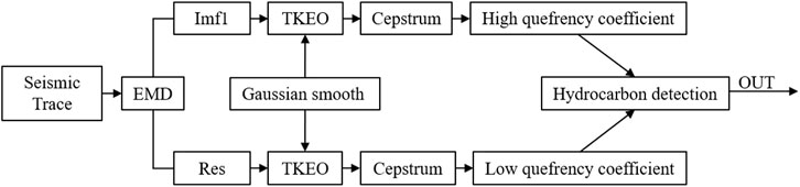
FIGURE 1. The algorithm flow chart.
Examples
Marmousi2 model
Low-frequency shadowing technology can effectively indicate the gas content of sandstone, that is, the difference between high and low frequencies. This phenomenon lays the foundation for the method proposed in this paper. Here, the Marmouis2 model was used as an example to verify the feasibility of the proposed EMD-TKE-Cepstrum method. The gas zone indicated by the arrow in Figure 2 exhibits a Class III gas-filled sand reservoir, which is brighter than the nearby events.
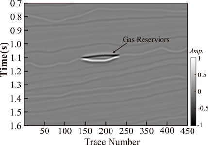
FIGURE 2. Seismic section.
In order to explain the principle and process of the algorithm step by step, we select the 180th seismic data as an example. As shown in Figure 3A, there was a strong gas-bearing response feature at 1.1 s. The IMF1 component shown in Figure 3B and the residual component shown in Figure 3C were decomposed by EMD. Spectral analysis was carried out for these three data sets, as shown in Figures 3D–F, respectively. The IMF1 component obviously contained the most high-frequency information, while the residual contained low-frequency information.
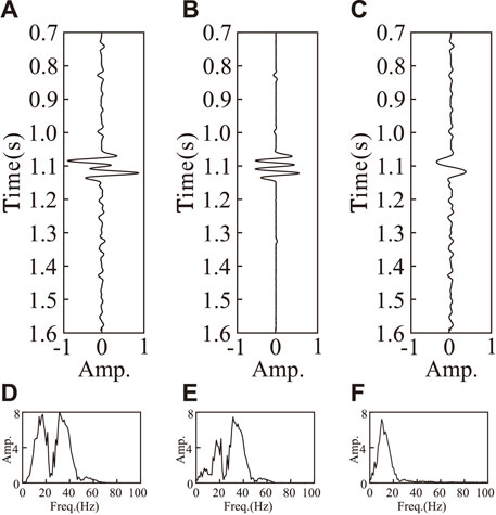
FIGURE 3. (A): Original seismic data, (B): IMF1 component, (C): residual, (D): spectrum diagram of a, (E): spectrum diagram of b, and (F): spectrum diagram of c.
The TKEO calculation was then performed. Figure 4A shows the IMF1 component calculated by TKEO, which was more instantaneous than the original data and was more focused to the target area. Figure 4B shows the result of the TKEO calculation. It is worth noting that the TKEO is sensitive to the instantaneous signal, so here it showed low-frequency noise in the quantity.
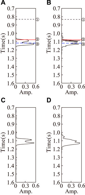
FIGURE 4. (A): Calculation results of IMF1 component TKEO, (B): calculation results of residual component TKEO, (C): calculation results of cepstrum coefficient of a, and (D): calculation results of cepstrum coefficient of c.
The cepstrum coefficient was calculated for the data after the TKEO calculation. First, we use the time window length of 8 sampling points; the data points are framed to obtain multiple signals. Each signal corresponds to a time point; we selected three different characteristics of the time point for experimental analysis. In Figures 4A,B, for ①②③ points, ① is the time point without gas, ② is the time point of the gas edge, and ③ is the time point of gas region; the frame length is eight. Figure 5A shows the single frame signal schematic of the IMF1-corresponding time point, while Figure 5C shows the single frame signal schematic of the residual-corresponding time point. The cepstrum calculation was then carried out, where Figure 5B shows the IMF1 component single-frame cepstrum result. It can be seen that the cepstrum domain transformation was slower without gas, and that the change with gas was faster than that without gas. Figure 5D shows the result of the residual component single frame cepstrum domain; the gas-free region showed the same result, whereas the gas content changed faster than the gas-free region, opposite to the result shown in Figure 5B. The first and second points in the cepstrum domain were selected for slope extraction to characterize the cepstrum coefficient. The cepstrum coefficient calculated by the IMF1 component is shown in Figure 4C; it exhibited relatively low results in the gas-bearing area, with relatively high results at the gas-bearing edge. The residual results are shown in Figure 4D, revealing that the cepstrum coefficient was relatively high in the gas region and relatively low in the non-gas region. This result is consistent with the currently accepted fluid theory of “pass low frequency, block high frequency,” which provides a basis for gas-bearing interpretations.
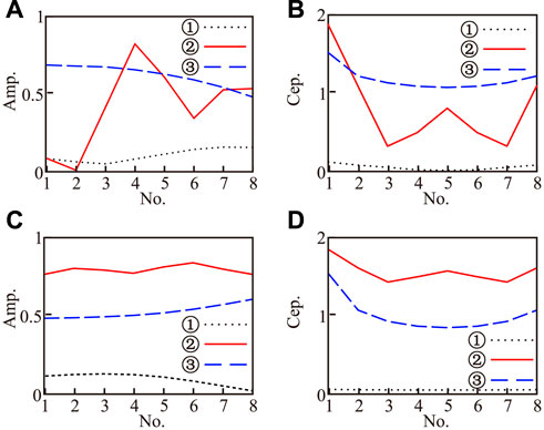
FIGURE 5. (A): Single frame of IMF1 after TKEO, (B). cepstrum coefficient of a, (C): single frame of residual after TKEO, and (D). cepstrum coefficient of c.
On the basis of the method presented above, the whole profile was calculated. Figure 6A shows the result of the IMF1 cepstrum coefficient, while Figure 6B shows the result of the cepstrum calculation of the residual profile. These results further confirm the phenomenon that the high frequency cepstrum coefficient was low and the low frequency cepstrum coefficient was high in the gas bearing area. At the same time, the high and low frequency sections of the model were extracted using the SCWT algorithm. Figure 7A shows the high frequency (45 Hz) result, while Figure 7B shows the low frequency (15 Hz) result. These calculation results also indicated the gas-bearing area, but the accuracy of this method was relatively low, and the edge and internal information of the gas-bearing reservoir were not marked.
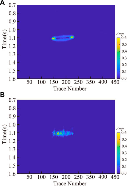
FIGURE 6. (A): IMF1 component cepstrum coefficient result profile and (B): residual component cepstrum coefficient result profile.
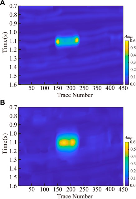
FIGURE 7. (A): 45 Hz common frequency sections obtained using SCWT method and (B): 15 Hz common frequency sections obtained using SCWT method.
Field data example
To further assess the ability of the proposed method to detect hydrocarbons, applied our approach to field data, as shown in Figure 8. These field data consisted of 1,400 traces, with 250 samples per trace and a time sampling interval of 2 ms. The profile data included well A and well B, and target layers T1 to T2. Well B contained gas wells, which were drilled into the gas layer as shown by the location of red ring (Figure 8.); well A was not drilled into the gas layer. The structural difference between these two wells was small, with similar seismic characteristics; these conditions greatly complicate the prediction of gas-bearing strata.
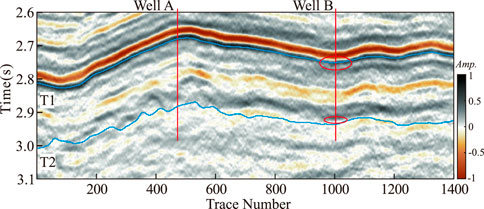
FIGURE 8. Seismic section.
Test and calculate the actual seismic data profile. The EMD algorithm separates the relatively high-frequency data from the relatively low-frequency data. Figure 9A shows the high-frequency components. It can be seen that the data phase axis is relatively fine, and the signal scale is small; Figure 9B shows the relatively low-frequency components. It can be seen that the signal scale is relatively large, mainly including the low-frequency components of the signal. TKEO calculation is carried out to improve the instantaneity of the signal. The high-frequency results are shown in Figure 9C, and the low-frequency results are shown in Figure 9D. It shows that the instantaneity of the signal is enhanced after TKEO calculation, and the difference between high and low frequencies is obvious, which is the subsequent cepstrum coefficient.

FIGURE 9. (A):IMF1 component, (B): Residual component, (C): TKEO of a, (D): TKEO of b.
Based on the above calculation, the cepstral coefficients of the actual data are calculated. The frame time window is selected as 16, and the number of coefficients is chosen as 3 to obtain the corresponding results. Figure 10A shows the calculation result of the high frequency component, while Figure 10B shows the calculation result of the section. These results show that in target layer T1, without gas well A, the high frequency cepstrum coefficient was strong. The low frequency cepstrum coefficient showed weak characteristics, meanwhile, and target layer T1 showed a weak response. Well B showed a strong high frequency cepstrum coefficient and a weak low frequency cepstrum coefficient at both the T1 and T2 target layers. The gas-bearing indication showed a strong high frequency cepstrum coefficient and a weak low frequency cepstrum coefficient, consistent with the overall gas-bearing distribution; this further confirms the effectiveness of the proposed method.
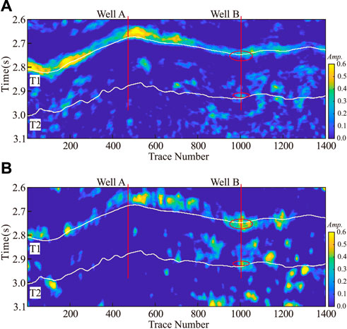
FIGURE 10. (A): Cepstrum coefficient profile of IMF1 component and (B): Cepstrum coefficient profile of Residual component.
At the same time, the SCWT method was used to extract high frequency sections (45 Hz), such as Figure 11A, and low frequency (15 Hz) sections, such as Figure 11B. The high and low frequency profiles show similar features to the results obtained using the proposed method, but the accuracy was relatively low. Especially in target layer T2, the gas content of well b was not shown, and the comparison showed the rationality and accuracy of the proposed method.
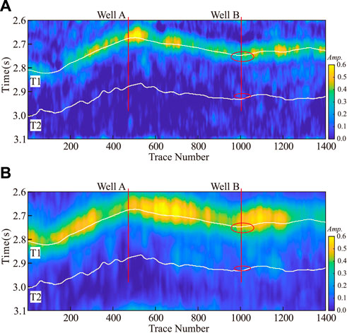
FIGURE 11. (A): 45 Hz common frequency sections obtained using SCWT method and (B): 15 Hz common frequency sections obtained using SCWT method.
Conclusion
We proposed a novel hydrocarbon detection approach using EMD-TKEO and cepstrum, termed EMD-TKE-Cepstrum. In this method, EMD adaptively decomposes the signal into the first component and the residual, representing the high and low frequency components, respectively. The TKEO, meanwhile, can directly enhance the instantaneousness of the component signal by focusing on its instantaneous characteristics. The cepstrum calculation then converts the signal into the cepstrum domain to improve the sensitivity of the signal-to-gas content. The cepstral coefficient transformation rate (slope) was here innovatively used as the cepstral coefficient to characterize the different characteristics of the gas content in high and low frequency components. This method is based on low-frequency shadow technology, which has higher focusing and clarity; it can highlight differences between high and low frequencies in gas-bearing areas while also improving the prediction accuracy. Here, model and field examples were used to validate the proposed method, with these results showing EMD-TKE-Cepstrum’s potential as a reservoir depiction tool for highlighting anomalies associated with hydrocarbons.
Data availability statement
The raw data supporting the conclusion of this article will be made available by the authors, without undue reservation.
Author contributions
All authors listed have made a substantial, direct, and intellectual contribution to the work and approved it for publication.
Funding
This work was supported by the National Natural Science Foundation of China (Grant Nos. 42030812, 41974160 and 42042046), China Postdoctoral Science Foundation (Grant No. 2022M710495), project of the SINOPEC Science and Technology Department (Grant No. P20055-6).
Conflict of interest
The authors declare that the research was conducted in the absence of any commercial or financial relationships that could be construed as a potential conflict of interest.
Publisher’s note
All claims expressed in this article are solely those of the authors and do not necessarily represent those of their affiliated organizations, or those of the publisher, the editors and the reviewers. Any product that may be evaluated in this article, or claim that may be made by its manufacturer, is not guaranteed or endorsed by the publisher.
References
Boudraa, A.-O., and Salzenstein, F. (2018). Teager–kaiser energy methods for signal and image analysis: A review. Digit. Signal Process. 78, 338–375. doi:10.1016/j.dsp.2018.03.010
Chen, Y., and Fomel, S. (2018). EMD-seislet transform. Geophysics 83, A27–A32. doi:10.1190/geo2017-0554.1
de Matos, M. C., Marfurt, K. J., Johann, P. R. S., Rosseto, J. A., Lourenço, A. T. A., and Diniz, J. L. (2009). Wavelet transform teager-kaiser energy applied to a carbonate field in Brazil. Lead. Edge 28, 708–713. doi:10.1190/1.3148413
Dragomiretskiy, K., and Zosso, D. (2014). Variational mode decomposition. IEEE Trans. Signal Process. 62, 531–544. doi:10.1109/tsp.2013.2288675
Fawad, M., Hansen, J. A., and Mondol, N. H. (2020). Seismic-fluid detection-a review. Amsterdam: Earth-Science Reviews, 210, 103347. doi:10.1016/j.earscirev.2020.103347
Gao, J., Song, Z., Gui, J., and Yuan, S. (2020). Gas-bearing prediction using transfer learning and cnns: An application to a deep tight dolomite reservoir. IEEE Geosci. Remote Sens. Lett. 19, 1–5. doi:10.1109/lgrs.2020.3035568
Hu, J.-s., Yang, S.-X., and Ren, D.-q. (2008). Study on the method of emd-based vibration signal time-frequency analysis. J. Vib. Shock 27, 71–154.
Jiang, X.-d., Cao, J.-x., Hu, J.-t., Xiong, X.-c., and Liu, J. (2020b). Pre-stack gather optimization technology based on an improved bidimensional empirical mode decomposition method. J. Appl. Geophys. 177, 104026. doi:10.1016/j.jappgeo.2020.104026
Jiang, X., Cao, J., Yang, J., Liu, J., and Zhou, P. (2020a). Avo analysis combined with teager-kaiser energy methods for hydrocarbon detection. IEEE Geosci. Remote Sens. Lett. 19, 1–5. doi:10.1109/lgrs.2020.3029170
Li, R., and He, D. (2012). Rotational machine health monitoring and fault detection using emd-based acoustic emission feature quantification. IEEE Trans. Instrum. Meas. 61, 990–1001. doi:10.1109/tim.2011.2179819
Liu, W., Cao, S., Wang, Z., Kong, X., and Chen, Y. (2017). Spectral decomposition for hydrocarbon detection based on vmd and teager–kaiser energy. IEEE Geosci. Remote Sens. Lett. 14, 539–543. doi:10.1109/lgrs.2017.2656158
Patil, A. T., Acharya, R., Patil, H. A., and Guido, R. C. (2022). Improving the potential of enhanced teager energy cepstral coefficients (etecc) for replay attack detection. Comput. Speech & Lang. 72, 101281. doi:10.1016/j.csl.2021.101281
Tian, R.-f., and Cao, J.-x. (2012). Seismic cepstral decomposition progressing technique. Prog. Geophys. 27, 1183–1188.
Tong, Z. Y., Dong, Z. Y., and Li, M. (2016). A new entropy bi-cepstrum based-method for dc motor brush abnormality recognition. IEEE Sens. J. 17, 745–754. doi:10.1109/jsen.2016.2635641
Wang, J., Fu, J., Xie, J., and Wang, J. (2020). Quantitative characterisation of gas loss and numerical simulations of underground gas storage based on gas displacement experiments performed with systems of small-core devices connected in series. J. Nat. Gas Sci. Eng. 81, 103495. doi:10.1016/j.jngse.2020.103495
Wang, Y., Huang, H., Yuan, S., Zhang, S., and Li, B. (2016). Gas prediction using low-frequency components of variable-depth streamer seismic data applied to the deepwater area of the south China sea. J. Nat. Gas Sci. Eng. 34, 1310–1320. doi:10.1016/j.jngse.2016.07.071
Xie, T., Zheng, X.-D., and Zhang, Y. (2016). Seismic facies analysis based on linear prediction cepstrum coefficients. Chin. J. Geophys. 59, 4266–4277.
Xue, Y.-j., Cao, J.-x., and Tian, R.-f. (2013). A comparative study on hydrocarbon detection using three emd-based time–frequency analysis methods. J. Appl. Geophys. 89, 108–115. doi:10.1016/j.jappgeo.2012.11.015
Xue, Y.-j., Cao, J.-x., Tian, R.-f., Du, H.-k., and Yao, Y. (2016). Wavelet-based cepstrum decomposition of seismic data and its application in hydrocarbon detection. Geophys. Prospect. 64, 1441–1453. doi:10.1111/1365-2478.12344
Xue, Y.-J., Du, H.-K., Cao, J.-X., Jin, D., Chen, W., and Zhou, J. (2018). Application of a variational mode decomposition-based instantaneous centroid estimation method to a carbonate reservoir in China. IEEE Geosci. Remote Sens. Lett. 15, 364–368. doi:10.1109/lgrs.2017.2788467
Xue, Y., Cao, J. x., and Tian, R. f. (2014). Emd and teager–kaiser energy applied to hydrocarbon detection in a carbonate reservoir. Geophys. J. Int. 197, 277–291. doi:10.1093/gji/ggt530
Yang, J., Lin, N., Zhang, K., Zhang, C., Fu, C., Tian, G., et al. (2021). Reservoir characterization using multi-component seismic data in a novel hybrid model based on clustering and deep neural network. Nat. Resour. Res. 30, 3429–3454. doi:10.1007/s11053-021-09863-z
Zayrit, S., Drissi, T. B., Ammoumou, A., and Nsiri, B. (2020). Daubechies wavelet cepstral coefficients for Parkinson’s disease detection. ComplexSystems. 29, 729–739. doi:10.25088/complexsystems.29.3.729
Keywords: hydrocabon, emd, cepstrum analysis, teager kaiser energy operator, reservioir
Citation: Jiang X, Cao J, Su Z, Fu J and Shi S (2022) Hydrocarbon detection based on empirical mode decomposition, teager-kaiser energy, and the cepstrum. Front. Earth Sci. 10:923173. doi: 10.3389/feart.2022.923173
Received: 19 April 2022; Accepted: 21 July 2022;
Published: 13 September 2022.
Edited by:
Tariq Alkhalifah, King Abdullah University of Science and Technology, Saudi ArabiaReviewed by:
Kamel Rahouma, Minia University, EgyptWei Liu, Beijing University of Chemical Technology, China
Copyright © 2022 Jiang, Cao, Su, Fu and Shi. This is an open-access article distributed under the terms of the Creative Commons Attribution License (CC BY). The use, distribution or reproduction in other forums is permitted, provided the original author(s) and the copyright owner(s) are credited and that the original publication in this journal is cited, in accordance with accepted academic practice. No use, distribution or reproduction is permitted which does not comply with these terms.
*Correspondence: Junxing Cao, Y2FvanhAY2R1dC5lZHUuY24=