Modeling Mesoscale Eddies Generated Over the Continental Slope, East Antarctica

Mesoscale eddies are abundant over the Antarctic continental slope, with the potential to regulate the water masses transport, mixing, and energy transfer. Over the relatively cold and fresh shelf regions around the Antarctic margins, in the absence of dense overflows, the baroclinic instability of the Antarctic Slope Current is still favorable in the generation of mesoscale eddies. However, mesoscale eddies are barely observed over the fresh shelf regions due to the sparsity of in situ hydrographic observations. Based on an idealized eddy-resolving coupled ocean-ice shelf model, this study investigates the characteristics of mesoscale eddies and corresponding influences on the local hydrographic properties over the continental slope, East Antarctica. With the aid of an automated eddy detection algorithm, bowl-shaped eddies are identified from the simulated velocity vector geometry. The Cyclonic Eddies (CE) has a barotropic vertical structure extending to more than 2,500 m depth, while the vertical shear of the Anticyclonic Eddies (AE) velocity is strong at the upper 200 m layer. Mesoscale eddies can trap the cold and fresh water in the southern flank of the Antarctic slope front and flow offshore to the relatively warm and saline region. Therefore, the influences of eddies on the hydrographic properties are not only governed by the eddy polarities but also the eddy-induced heat and salt transport.

1 Introduction

Mesoscale eddies are ubiquitous in the World Ocean (Mcwilliams, 2008), with unique features in the Antarctic marginal sea. Based on the sea-surface height constructed from the merged TOPEX/Poseidon (T/P) and ERS-1/2 altimeter datasets, the observed mesoscale eddies account for more than 50% of the variability of the sea-surface height over much of the World Ocean (Chelton et al., 2007), with the time-scale ranging from just a few days to several months and the spatial-scale ranging from a few kilometers to more than 100 km (Mcwilliams, 2008; St-Laurent et al., 2013; Gunn et al., 2018). According to the direction of rotation, mesoscale eddies are classified as Cyclonic Eddies (CE) and Anticyclonic Eddies (AE). In the southern hemisphere, mesoscale eddies with larger amplitude and stronger rotational speeds are preferentially cyclonic (Chelton et al., 2011). The horizontal spatial-scale of mesoscale eddies is largely determined by the first baroclinic Rossby radius of deformation R₁, which is the ratio of the long gravity wave speed to the Coriolis frequency. Since R₁ can be less than 10 km around the Antarctic continental slope (Chelton et al., 1998), mesoscale eddies intend to have a relatively small spatial-scale in the Antarctic marginal sea.

Around the Antarctic marginal sea, the westward Antarctic Slope Current (ASC) almost encircles the Antarctic continent (Thompson et al., 2018), coupled with a sharp frontal zone, the Antarctic Slope Front (ASF). Over the steep continental slope, the isopycnal tilting of the ASF is typically largest at the shelf break, acting as an effective potential vorticity barrier to prevent the cross-slope exchanges of water masses (Bower et al., 1985). Meanwhile, as an extensive and coherent current, the ASC also has the potential to mediate the exchanges of water masses across the ASF. The onshore heat transport across the ASF can increase the heat content of shelf waters and accelerate the basal melting of the ice shelves (Shepherd et al., 2004; Pritchard et al., 2012; Rignot et al., 2013), whereas the offshore export of dense shelf water directly sets the production and properties of Antarctic Bottom Water that supplies the deep branch of the global overturning circulation (Moffat et al., 2009; Nøst et al., 2011). In addition, the ASC can regulate the cross-slope transport of nutrients and phytoplankton in the Antarctic continental slope area (Prézelin et al., 2000; Prézelin et al., 2004; Heywood et al., 2014; Wadley et al., 2014). Such cross-slope exchanges of water masses are closely associated with the structure and variability of the ASC. The ASC features a turbulent frontal current, with its abundance of jets and mesoscale eddies (Stern et al., 2015; Stewart and Thompson, 2015; Peña-Molino et al., 2016; Stewart and Thompson, 2016; Azaneu et al., 2017). The jets in the ASC are generally constrained by the gradient of the slope, yet these jets can be very unstable and drift northward when the vertical velocity shear reaches the critical condition for the baroclinic instability (Stern et al., 2015). The energetic mesoscale eddies over the shelf break are closely associated with the dense shelf water outflows across the ASF and substantially contribute to the Antarctic overturning circulation in the Weddell and Ross Seas (Stewart and Thompson, 2015; Stewart and Thompson, 2016).

The formation and migration of mesoscale eddies can trap the source water in their interior and transport the water downstream, with great significance in the cross-slope exchanges around the Antarctic margins. In the Southern Ocean, mesoscale eddies are a prevalent feature in the Antarctic Circumpolar Current (ACC) regime (Rintoul et al., 2001), with Circumpolar Deep Water (CDW) retained and transported southward across the ocean fronts to higher latitudes (Phillips and Rintoul, 2000). As warm CDW approaches the Antarctic continental slope, mesoscale eddies are favorable in the onshore advection of CDW onto the continental shelf (Moffat et al., 2009; Martinson and McKee, 2012; St-Laurent et al., 2013; St-Laurent et al., 2013). Meanwhile, mesoscale eddies also favor the offshore overflows of dense shelf water from the Antarctic continental shelf (Stewart and Thompson, 2012; Stewart and Thompson, 2013; Su et al., 2014; Dufour et al., 2017). The residual-mean theories suggest a leading-order balance between wind-induced and eddy-induced overturning circulations in the Southern Ocean (Marshall and Speer, 2012), and such a structure is also active at the Antarctic marginal seas (Nøst et al., 2011; Stewart and Thompson, 2013; Hattermann et al., 2014). Based on the hydrographic observations from ocean gliders, the eddy-induced overturning circulation is almost comparable to the wind-forced overturning cell in the northwestern Weddell Sea (Thompson et al., 2014). Therefore, the eddy-resolving horizontal resolution of numerical models is needed to simulate the contribution of mesoscale eddies to cross-slope exchanges of water masses (St-Laurent et al., 2013).

The rotations of mesoscale eddies can laterally stir the nearby waters and result in significant mixing and energy transfer. The lateral stirring of mesoscale eddies is expected to play a role in eroding the ocean fronts, e.g., the ASF, converting the available potential energy to kinetic energy. The cyclonic (anticyclonic) rotational eddies also contribute to the vertical mixing by giving rise to the upwelling (downwelling), and thereby eddies can enhance the primary production by bringing nutrient-rich water from the deeper layer to the sea surface (Kahru et al., 2007; Gaube et al., 2014; McGillicuddy, 2016). Generally, the energy cascade is from large scales to small scales, yet mesoscale eddies can also transfer energy from high baroclinic mode to low baroclinic and barotropic modes (Charney, 1971; Ferrari and Wunsch 2009). The eddy kinetic energy stems from the mean kinetic energy and the eddy potential energy by the barotropic conversion and baroclinic conversion (Lorenz, 1955; Kang and Curchitser, 2015). Over the Antarctic continental slope in Prydz Bay, the source of eddy kinetic energy is found to be provided by the baroclinic conversion rather than the barotropic conversion (Liu et al., 2018).

Mesoscale eddies mostly arise from the barotropic and baroclinic instabilities (Charney 1947; Eady 1949). In the western Weddell Sea, the observed dense overflows on the continental slope are found to be responsible for the generation of eddies (Baines and Condie 1998), and such effects of the dense fluid descending on a slope have been replicated in a variety of laboratory experiments (Lane-Serff and Baines 1998). High-resolution regional models have subsequently captured the periodic formation of eddies induced by dense water plumes over the Antarctic continental slope by resolving the mesoscale processes (Wang et al., 2009; Nakayama et al., 2014). Therefore, both observational and modeling studies have documented the energetic mesoscale eddy field hosted by the Antarctic continental slope. However, despite the baroclinic instability induced by dense overflows (Stewart and Thompson, 2016), the ASC may evolve in a baroclinically unstable state (Stern et al., 2015). As a frontal current steered by the steep continental slope, the velocity field of the ASC has strong lateral and vertical shear in facilitating the genesis of mesoscale eddies (Nøst et al., 2011; Hattermann et al., 2014). Compared to the mesoscale eddies induced by the dense overflows, our understanding of the mesoscale eddies directly fueled by the baroclinic instability of the ASC remains remarkably unknown.

In order to investigate the mesoscale eddies generated by the baroclinic instability of the ASC, we intend to focus on the Antarctic marginal sea where there are no dense water plumes over the continental slope. Based on the hydrographic properties, a classification of the ASC/ASF structure has been introduced as three cases: (I) Fresh Shelf, (II) Dense Shelf, and (III) Warm Shelf (Thompson et al., 2018). The mesoscale eddies induced by dense overflows over the slope are concentrated over the Dense Shelf regions where the Antarctic Bottom Water are produced (Orsi et al., 1999; Whitworth and Orsi, 2006). To exclude the influences of such dense overflows, this study focuses on the mesoscale eddies over Fresh Shelf regions. Over Fresh Shelf regions, the ASF is characterized by the intense lateral density gradient over the slope, and such a strong frontal structure can effectively separate the warm deep water from the cold shelf water. The strong ASF over Fresh Shelf regions stems from a combination of weak cross-slope exchange, Ekman downwelling, and the presence of cold shelf waters (Thompson et al., 2018). Therefore, the Fresh Shelf can exhibit the influences of ASC baroclinic instability and corresponding eddy generation, without the influences of dense overflows.

The spatial structure of mesoscale eddies and corresponding influences on the hydrographic parameters reveal the dominant characteristics of mesoscale eddies. Three different types of mesoscale eddies are classified based on the vertical shapes: (I) bowl-shaped eddies with the maximal radius at the surface, (II) lens-shaped eddies with the maximal radius at the middle depth, and (III) cone-shaped eddies with the maximal radius at the eddy bottom (Dong et al., 2012). The analysis of the eddy spatial structure has been extensively used in both observational studies and numerical simulations, and bowl-shaped eddies are widely prevalent (Martin et al., 1998; Qiu and Chen, 2010; Zhang et al., 2014; Lin et al., 2015). However, due to the limited hydrographic observations and the relatively small R₁ over the Antarctic continental slope, it is not easy to directly uncover the spatial structure of mesoscale eddies based on in situ observations. For example, over the continental shelf of the Ross Sea, the simulated spatial-scale of mesoscale eddies can have a minimum of ∼5 km (Mack et al., 2019). So far, Williams et al. (2010) documented a bowl-shaped eddy observed within the Prydz Bay Gyre region that is a typical Fresh Shelf case in East Antarctica. High-resolution numerical models shed light on the details of the dynamic structure of mesoscale eddies. With the aid of an idealized eddy-resolving model, this study intends to delineate the spatial structure of mesoscale eddies generated by the baroclinic instability of the ASC over Fresh Shelf regions.

In this study, an idealized eddy-resolving model is designed for a fresh shelf case in an effort to characterize the mesoscale eddies and associated hydrographic properties over the Antarctic continental slope. In Section 2, we describe the model configuration and the methods. The characteristics of mesoscale eddies and the eddy-induced anomalies in the hydrographic properties are illustrated in Section 3. Conclusions and discussions are provided in Section 4.

2 Model Configuration and Methodology

2.1 Model Configuration

Based on the Massachusetts Institute of Technology General Circulation Model (Marshall et al., 1997; Losch et al., 2010), our experiments are conducted with an idealized eddy-resolving coupled ocean-ice shelf model. The idealized topography configuration consists of a deep ocean area, a steep continental slope, a shallow continental shelf, a submarine trough, and an ice cavity (Figure 1A), with the geographic coordinate representing a typical Fresh Shelf region in East Antarctica. The orange boxes in Figure 1B show the locations of Prydz Bay (60°E–90°E) and the Sabrina Coast (110°E–125°E) that are the typical Fresh Shelf cases around East Antarctica (Figures 1C,D). The model horizontal resolution is 0.0125° and 0.005° in the zonal and meridional directions, respectively. Accordingly, the averaged zonal grid spacing is ∼554 m, and the meridional grid spacing is ∼555 m. Although R₁ could be less than 10 km over the continental slope, this high horizontal resolution is still able to properly resolve the mesoscale eddies. To capture the vertical structure of mesoscale eddies over the continental slope, the model has 70 levels in upper 700 m depth, 20 levels from 700 m depth to 1,700 m depth, and 10 levels from 1,700 m depth to 3,000 m depth, with uniform intervals of 10, 50 and 130 m, respectively.

FIGURE 1

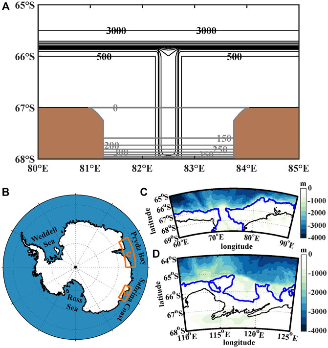
FIGURE 1. (A) Topographical features of the idealized coupled ocean-ice shelf model. The black lines are the seafloor depth (at 50 m intervals from 500 to 1,000 m, and 500 m intervals from 1,000 m to 3,000 m), and the grey lines are the ice shelf draft in contour intervals of 50 m. (B) The orange boxes in the map show the typical Fresh Shelf regions around East Antarctica, corresponding to (C) and (D), respectively. (C) The topography (m) in Prydz Bay, with the coastal line (black line) and the 500 m isobath (blue line). (D) Same as (C), but for the Sabrina Coast.

The open boundary conditions are used to force the ocean by prescribing the velocity, the potential temperature, and the salinity fields on the eastern, western, and northern boundaries (Figure 2). In order to focus on mesoscale eddies generated by the ASC and exclude the sea surface influences, e.g., eddies generated by sea ice leads (Cohanim et al., 2021), the sea ice model and the atmospheric forcing are not included. On the zonal open boundaries, the ASC is represented by a westward jet over the continental slope (Figure 2A). The jet velocity ranges from −0.3 m s⁻¹ at the surface layer to 0 at the bottom layer, and the meridional extension of the jet is confined within the continental slope. Such strong vertical and lateral shear of the ASC is in accordance with the geostrophic balance with the ASF. The ASF is represented by a sharp thermohaline front over the slope, with the thermocline and the halocline intersecting the upper slope. The values of the open boundary conditions are set to represent the typical hydrographic characteristics of a Fresh Shelf case on the basis of comprehensive observational data sets, including the mooring observations (Heywood et al., 1999; Peña-Molino et al., 2016), the instrumented southern elephant seal data (Treasure et al., 2017), and the Conductivity-Temperature-Depth vertical profile stations (Williams et al., 2010).

FIGURE 2

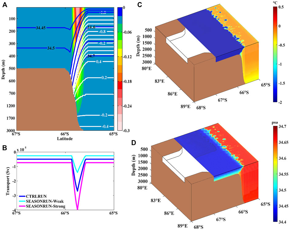
FIGURE 2. (A) The cross-section of the zonal open boundary conditions in the CTRLRUN. The color shading is the zonal velocity (negative westward/into the page); white lines are the potential temperature (°C) in contour intervals of 0.2°C; blue lines are the salinity (psu) in contour intervals of 0.05. (B) Cross-shelf variation of the vertical integrated zonal transport (Sv). (C) A snapshot of the potential temperature (°C) in the CTRLRUN, the top layer is at 100 m depth. (D) Same as (C), but for the salinity (psu).

The model is integrated for 3 years with the open boundary forcing that is held constant, denoted the CTRLRUN. In the CTRLRUN, the initial conditions are zonally uniform for each depth level, with values equal to that on the zonal open boundaries. After integration of 2 years, the simulation reaches the quasi-equilibrium status, and we use the 6-h mean outputs in the third year to investigate the structure of mesoscale eddies over the slope. A sensitivity experiment is initialized from the final output of the CTRLRUN, denoted by the SEASONRUN, with the same open boundary conditions for the potential temperature and salinity. In the SEASONRUN, a sinusoidal pulsing with a yearly period is added to the original zonal velocity to represent the seasonal cycle of the ASC on the basis of mooring observations (Heywood et al., 1999; Mathiot et al., 2011; Peña-Molino et al., 2016). The amplitude of the sinusoidal pulsing is half of the original zonal velocity in the CTRLRUN, and the maximal magnitude of the ASC is set on June 30th. The SEASONRUN is integrated for 3 years and reaches the quasi-equilibrium status in the second year, and the 6-h mean outputs in the third year are saved to investigate the influences of the ASC seasonality on mesoscale eddies. The simulated results during the period from June to July in the SEASONRUN are used to represent the strong ASC in winter, denoted by the SEASONRUN-Strong, and the period from Dec to Jan in the SEASONRUN is used to represent the weak ASC in summer, denoted by the SEASONRUN-Weak (Figure 2B).

The presence of mesoscale eddies can be directly revealed via the eddy eroding effects on the ASF. The ASF in this idealized model is characterized by a sharp front separating the warm and saline modified Circumpolar Deep Water (mCDW) from the cold and fresh Shelf Water (SW). The lateral eddy stirring between the mCDW and SW is clearly visible from the snapshots of the potential temperature and the salinity, with cold and fresh eddy boluses of SW in the northern flank of the ASF (Figures 2C,D).

2.2 Eddy Detection Scheme

In this study, we adopt an automated eddy detection algorithm that is based on the vector geometry method (Nencioli et al., 2010). This algorithm has been extensively used to detect eddies in the open ocean and marginal seas (Couvelard et al., 2012; Peliz et al., 2013; Dong et al., 2014; Sun et al., 2017; Sun et al., 2021a, 2021b). From the perspective of an observer moving with the temporal-averaged current, an eddy can be recognized as a flow structure that the relative velocity vectors encircle a center of the minimum magnitude. Within such a circle, the tangential velocity should increase with distance from the eddy center and then decays after reaching a maximum.

To be in accordance with the characteristics of the eddy velocity field, four constrains are proposed by the vector geometry method: (I) the minimal velocity magnitude should be located in the eddy center; (II) along a zonal cross-section, the meridional velocity should have opposite signs over the different sides of the eddy center; (III) along a meridional cross-section, the zonal velocity should have opposite signs over the different sides of the eddy center, with the same rotational direction as the meridional velocity; (IV) the rotational direction of the velocity vector should be constant around the eddy center, and the two neighboring velocity vectors should point to the same or two adjacent quadrants. Two parameters need to be specified for the application of the vector geometry method. The first parameter, a, determines the grid numbers that will be checked away the increases in the magnitude of the zonal velocity along the meridional axis and the meridional velocity along the zonal axis. The parameter a also determines a counter along which the changes in the velocity vector direction are checked. The second parameter, b, determines the dimension of a domain used to locate the local minimal velocity magnitude. Optimal values for a and b are largely dependent on the spatial resolution of the dataset. In order to reduce the failure and excess rate of the eddy detection, we conduct a series of sensitivity tests and specify a = 7 and b = 6 for an optimal algorithm performance. When an eddy center is located, the boundary of the eddy is computed as the largest local stream function counter encircling the eddy center. The eddy radius is computed as the averaged distance from the outmost boundary points to the eddy center. Compared with the Okubo–Weiss and Winding Angle methods (Nencioli et al., 2010), this vector geometry method has a better successful identification rate and a lower excessive identification rate.

2.3 Eddy Composition and Statistical Analysis

In order to reveal the typical characteristic of mesoscale eddies over the continental slope, the composite analysis method is used to derive a uniform eddy structure (Sun et al., 2018). According to the polarity, mesoscale eddies are classified as two different types: the CE and the AE. Based on the eddy detection results, the detected eddy domain is converted from the geographic coordinate (∇x, ∇y) to a normalized coordinate system (∇X, ∇Y) as:

$\nabla X=\frac{\nabla x}{R_e} (1)$

$\nabla Y=\frac{\nabla y}{R_e} (2)$

where ∇x and ∇y are the zonal and meridional geographic distance of the grid to the eddy center, ∇X and ∇Y are the normalized distance of the grid to the eddy center, and R_e is the corresponding eddy radius. The resolution for the normalized coordinate is set as 0.05 in this study. As the eddy centers are all placed at the origin point of the normalized coordinate, we can construct a composite eddy field for the CE/AE by averaging the values at the same normalized location. By conducting such a composite analysis for every vertical level, a composite spatial structure of mesoscale eddies can be derived for the CE/AE.

In order to have a clear statistical analysis of the eddy field, we also calculate the averaged values along a set of concentric circles around the composite eddy center as follows: (I) the composite eddy domain is further discrete by a set of concentric circles with a uniform increase of 0.1 in the radius; (II) the grids in a track bounded by two adjacent concentric circles are selected for every track; (III) the averaged value over the selected grids in a track is calculated and assigned to the corresponding track. Such a statistical analysis of the eddy field serves to smooth out the local disturbances and preset the more straightforward horizontal structure of a composite eddy.

The study uses the anomalies of the simulated outputs for the eddy detection and composition. The anomalies of the CTRLRUN are derived by the deviation from the annual mean. The anomalies of the SEASONRUN-Strong are derived by the deviation from the temporal average from December and January, and the anomalies of the SEASONRUN-Strong are derived by the deviation from the temporal average from June and July.

3 Results

3.1 Eddy Detection

From the snapshots of the potential temperature and the salinity, mesoscale eddies are mostly active in the northern flank of the ASC over the lower continental slope (Figures 2C,D). For a Fresh Shelf case where there are no dense overflows, it is reasonable to expect that the mesoscale eddies are less evident over the upper continental slope due to the suppression of the strong topographic vorticity gradient (Isachsen, 2011; Stewart and Thompson, 2013). Since the mesoscale eddies generated by the baroclinic instability of the ASC are concentrated along the northern flank of the ASC (Figures 2C,D), the alternatively positive and negative values dominate the horizontal velocity over the lower slope (Figures 3A,B), resulting in the water swirling around the eddy center. In good agreement with the velocity field, the potential temperature (salinity) also shows alternatively warm (saline) and cold (fresh) water boluses over the lower slope, implying the eddy-induced cross-front transport (Figures 3C,D).

FIGURE 3

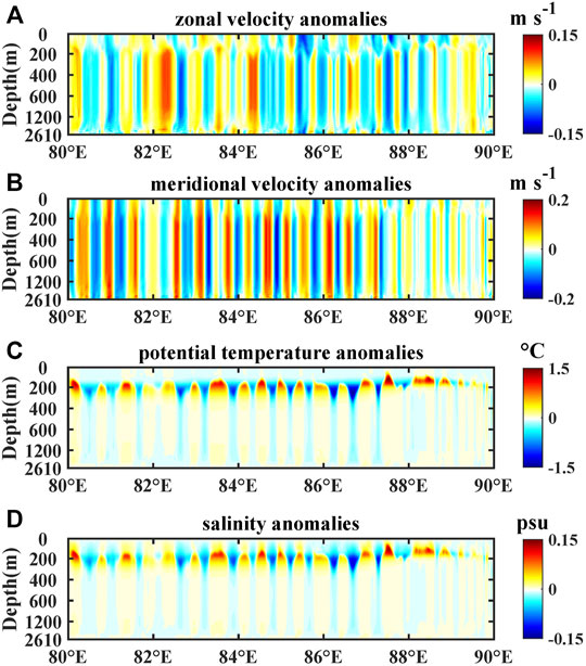
FIGURE 3. (A) A snapshot of the zonal cross-section (65.7°S) of the zonal velocity anomalies (m s⁻¹) at the lower continental slope (seafloor depth is 2,610 m). (B–D) Same as (A), but for the meridional velocity anomalies (m s⁻¹), the potential temperature anomalies (°C), and the salinity anomalies (psu), respectively.

With the aid of the eddy detection scheme, energetic mesoscale eddies are identified from the surface velocity fields (Figure 4A), and the sea surface height also shows a quite good congruence with the polarities of mesoscale eddies, with negative (positive) anomalies corresponding to the CE (AE). For a specific identified mesoscale eddy (Figure 4B), the detection scheme provides the location of the eddy center, the eddy shape, the eddy lifetime from its generation to termination, and the eddy trajectory.

FIGURE 4

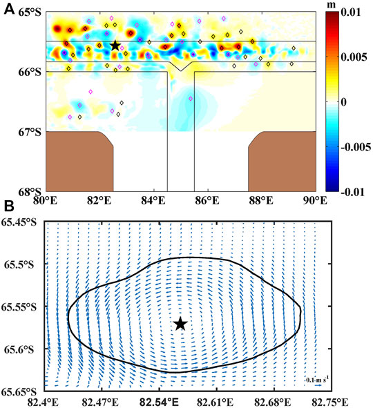
FIGURE 4. (A) A snapshot of eddy centers detected by the vector geometry method. The black diamonds are the detected CE, and the magenta diamonds are the detected AE. The color shading is sea surface height anomalies. The thin black lines denote the isobaths of 500, 700, and 3,000 m from south to north. The black star denotes an anticyclonic eddy shown in (B). (B) The snapshot of an anticyclonic eddy with sea surface velocity vectors in units of m s⁻¹. The black line denotes the boundary of the detected anticyclonic eddy.

3.2 Spatial Structures of Composite Eddies

Based on the eddy composition method, the spatial structures of the composite eddies are derived from all the CE and the AE detected by the vector geometry method. Both the composite CE and AE show bowl-shaped structures in the CTRLRUN, with an almost symmetric structure to the eddy center (Figures 5A,B). Both the composite CE and AE have a similar thickness of ∼2,500 m. However, the composite eddy velocity of the CE almost does not change from the sea surface to more than 2,500 m depth, while the composite eddy velocity of the AE rapidly decreases in the upper 200 m layer. As expected, the minimal velocity magnitude is still located at the composite eddy centers from the surface layer to the bottom layer (Figures 5A,B). At the sea surface layer, the magnitude of the composite velocity vectors gradually increases with the distance to the eddy center to a maximum and then decreases toward the eddy boundary (Figures 5C,D). The averaged radius of CE is ∼8.5 km, and the averaged radius of AE slightly larger than that of CE, with an averaged value of ∼9.8 km.

FIGURE 5

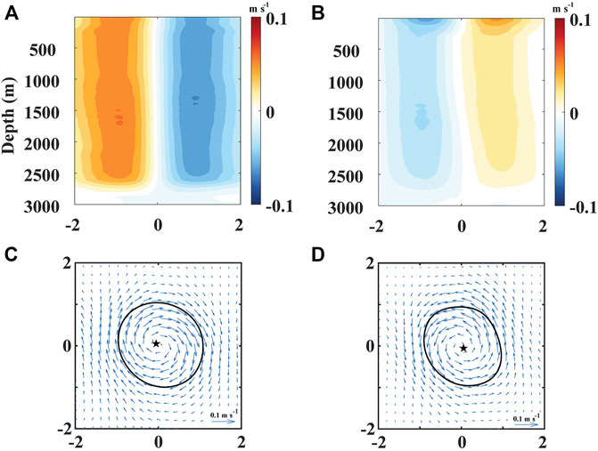
FIGURE 5. (A) The zonal cross-section of composite meridional velocity anomalies of the CE across the eddy center in the CTRLRUN. (B) Same as (A), but for the composite eddy of AE. (C) Horizontal distribution of composite velocity vector anomalies of the CE at the surface layer in the CTRLRUN. (D) Same as (C), but for the composite eddy of AE.

3.3 Hydrographic Anomalies Associated With Composite Eddies

Mesoscale eddies can induce significant changes in the potential temperature, the salinity, and the potential density of water masses. Since the rotation of mesoscale eddies can lead to local upwelling or downwelling, the vertical structure of hydrographic properties should change in response to the polarity of mesoscale eddies. As the deep water is warmer, saltier, and denser than the water in the upper layer over the continental slope (Figures 6A–C), the composite eddy of CE is expected to be associated with the positive potential temperature and salinity anomalies, while the composite eddy of AE is expected to be associated with the negative anomalies. However, the transport of the water masses trapped within the eddy can also induce hydrographic anomalies downstream. Therefore, it is reasonable to find that hydrographic properties may have complex changes in response to mesoscale eddies, especially near a sharp frontal zone.

FIGURE 6

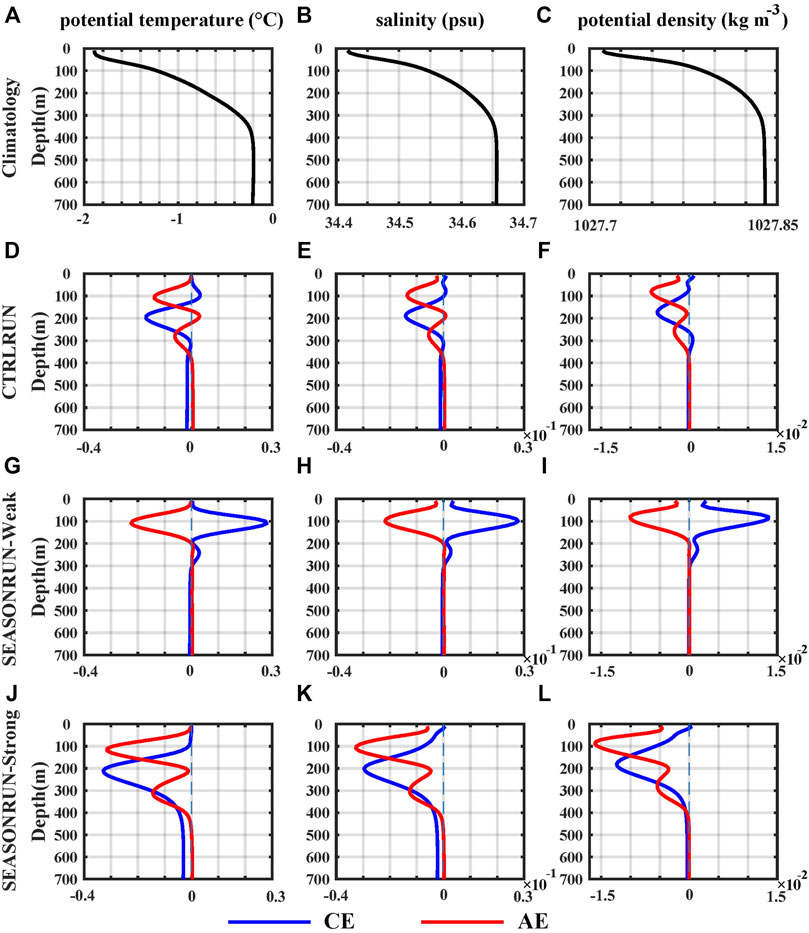
FIGURE 6. (A–C) Vertical profiles of the temporal averaged potential temperature (°C), salinity (× 10⁻¹ psu), and potential density (× 10⁻² kg m⁻³) in the CTRLRUN over the lower continental slope. Vertical profiles of the anomalies within the composite eddies in the CTRLRUN, for the potential temperature (D), the salinity (E), and the potential density (F). (G–I) Same as (D–F), but for the composite eddies in the SEASONRUN-Weak. (J–L) Same as (D–F), but for the composite eddies in the SEASONRUN-Strong. Blue lines are the anomalies of the composite eddies of the CE, and red lines are the anomalies of the composite eddies of the AE.

Within the composite eddy of the CE from the CTRLRUN, a cooling peak of ∼−0.17°C presents at 200 m depth (Figure 6D), with a maximal salinity change of ∼−0.14 × 10⁻¹ psu at 190 m depth (Figure 6E). Accordingly, the maximal potential density change of ∼−0.5 × 10⁻² kg m⁻³ also presents at 180 m depth (Figure 6F). Compared to the CE, the composite eddy of AE has two cooling peaks (Figure 6D). The maximal potential temperature change of ∼−0.14°C is at 110 m depth (Figure 6D), with a maximal salinity change of ∼−0.14 × 10⁻¹ psu at 100 m depth (Figure 6E). The second cooling peak of ∼−0.6 × 10⁻¹°C is at ∼280 m depth (Figure 6D), with a maximal salinity change of ∼0.6 × 10⁻² psu at ∼280 m depth (Figure 6E). Two negative peaks of the potential density anomalies are also present at 80 and 260 m depths (Figure 6F), closely consistent with the potential temperature and the salinity anomalies. As the transport of the ASC decreases in the SEASONRUN-Weak, for the composite eddy of CE, a warm peak of ∼0.28°C presents at ∼110 m depth (Figure 6G), with a maximal salinity change of ∼0.27 × 10⁻¹ psu at ∼100 m depth (Figure 6H). Accordingly, the maximal potential density change of 0.14 × 10⁻¹ kg m⁻³ presents at ∼90 m depth (Figure 6I). For the composite eddy of AE from the SEASONRUN-Weak, the negative peaks of the potential temperature, salinity, and potential temperature in the deeper layer vanish. An intensified cold peak of ∼−0.23°C presents at ∼110 m depth (Figure 6G), with a maximal salinity change of ∼−0.22 × 10⁻¹ psu at 100 m depth (Figure 6H). The maximal potential density change of ∼−0.1 × 10⁻¹ kg m⁻³ presents at 80 m depth (Figure 6I). As the transport of the ASC increases in the SEASONRUN-Strong, a cooling peak of ∼−0.33°C presents at 210 m depth (Figure 6J), with a maximal salinity change of ∼−0.3 × 10⁻¹ psu at 200 m depth (Figure 6K). Accordingly, the maximal potential density change of ∼−0.12 × 10⁻¹ kg m⁻³ also presents at 180 m depth (Figure 6L). For the composite eddy of AE in the SEASONRUN-Strong, two negative peaks are present in the anomalies of the potential temperature, the salinity, and the potential density (Figures 6J–L). The maximal change of potential temperature is ∼−0.32°C is at 120 m depth (Figure 6J), with a maximal salinity change of ∼−0.33 × 10⁻¹ psu at 110 m depth. The second peak of ∼−0.14°C is at ∼310 m depth (Figure 6K), with a maximal salinity change of ∼0.13 × 10⁻¹ psu at ∼300 m depth (Figure 6K). Two negative peaks of the potential density anomalies are present at 90 and 280 m depths (Figure 6L), with a maximal of ∼−0.16 × 10⁻¹ kg m⁻³ at 90 m depth.

Since the influences of the composite eddies on hydrographic properties are almost negligible below 500 m depth (Figure 6), we show the vertical structure of the composite eddies in the upper 500 m layer (Figure 7). In the CTRLRUN, the zonal cross-sections across the composite eddy centers show that the influences of mesoscale eddies on hydrographic properties are mainly limited to the upper 300 m layer (Figures 7A–F). In consistent with the vertical profiles shown in Figure 6, the composite negative centers of the CE are located around the 200 m depth (Figures 7A–C), while the composite anomalies of the AE have double negative centers sitting at ∼100 and ∼300 m depths for all hydrographic properties (Figures 7D–F). The horizontal extensions of these anomalies are mainly confined with 1 radius of the composite eddies for both the CE and the AE. In the SEASONRUN-Weak, the remarkable warmer, saltier, and denser anomalies are present in the composite eddy of the CE at ∼100 m depth (Figures 7G–I), with upward-pointing triangle structures. In contrast, the remarkable colder, fresher, and lighter anomalies present in the composite eddy of AE at ∼100 m depth (Figures 7J–L), with downward-pointing triangle structures. The horizontal extension of the AE is still confined with 1 radius, yet the composite influences of the CE can reach 2 radii. In the SEASONRUN-Strong, the composite negative anomalies of the CE dominate the maximal changes of potential temperature, the salinity, and the potential density at ∼200 m depth, with downward-pointing triangle structures (Figures 7M–O). Similar to the composite eddy of AE in the CTRLRUN, double negative centers are present in the composite anomalies of the AE in the SEASONRUN-Strong, with downward-pointing triangle structures centered at ∼100 and ∼300 m depths (Figures 7P–R). The spatial structures of the eddy-induced anomalies in the SEASONRUN-Strong are analogous to that in the CTRLRUN, but the responses of hydrographic properties are more significant when the transport of the ASC is stronger.

FIGURE 7

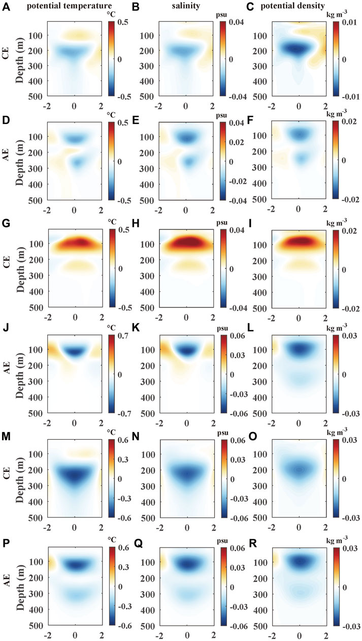
FIGURE 7. (A) The zonal cross-section of the potential temperature (°C) anomalies of the composite eddy of the CE across the eddy center in the CTRLRUN. (B) Same as (A), but for the salinity (psu) anomalies. (C) Same as (A), but for the potential density (kg m⁻³) anomalies. (D–F) Same as (A–C), but for the composite eddy of the AE at 100 m depth in the CTRLRUN. (G–L) Same as (A–F), but for the composite eddies of the CE and the AE in the SEASONRUN-Weak. (M–R) Same as (A–F), but for the composite eddies of the CE in the SEASONRUN-Strong.

Based on the statistical analysis that averages the values along a set of concentric circles around the composite eddy center at a constant depth, the local disturbances are smoothed out to further depict the horizontal structure of the composite eddies (Figure 8). Generally, the influences of the composite eddies should weaken with the increasing distance from the eddy centers and almost vanish at the eddy boundaries; however, the anomalies may not decay linearly from the composite eddy center to the eddy boundary.

FIGURE 8

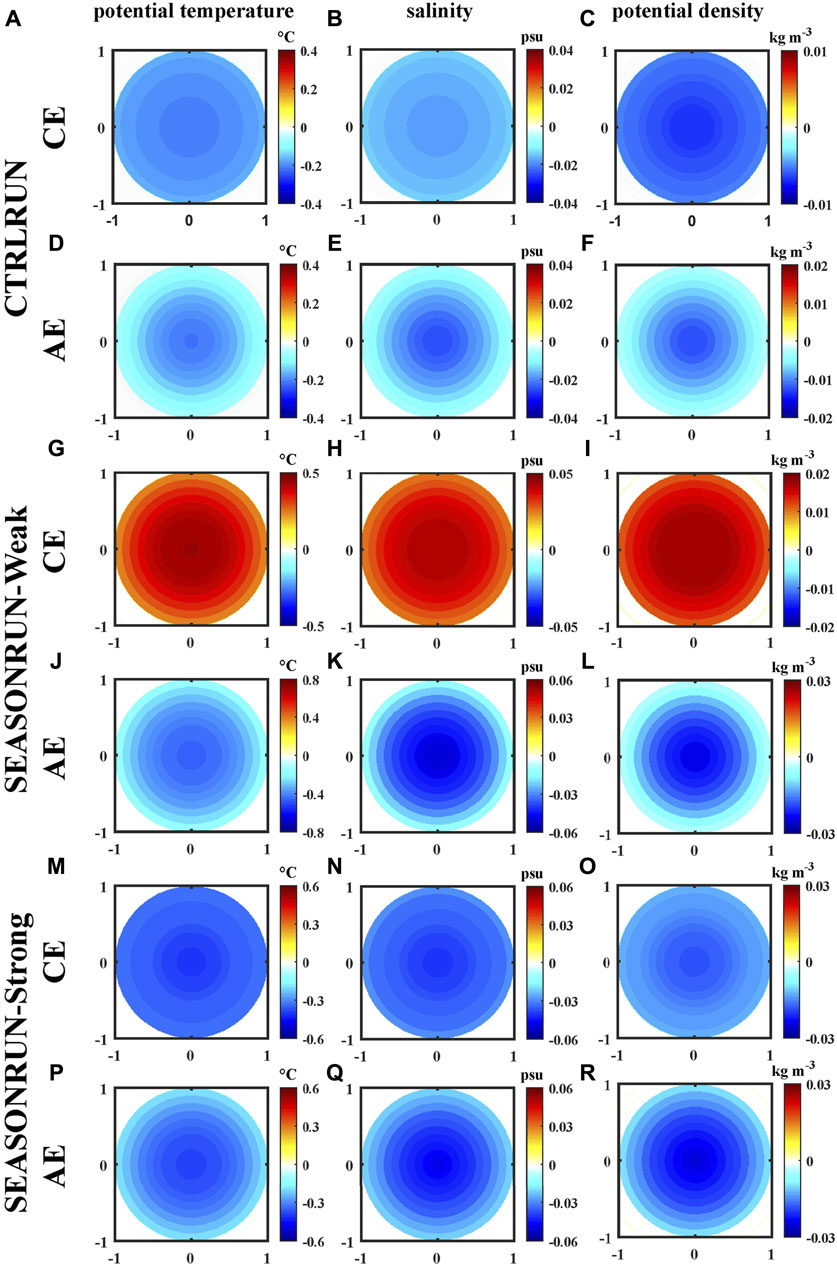
FIGURE 8. (A) The averaged values of potential temperature anomalies (°C) along a set of concentric circles around the composite eddy center of CE at 200 m depth in the CTRLRUN. (B) Same as (A), but for the salinity anomalies (psu). (C) Same as (A), but for the potential density anomalies (kg m⁻³). (D–F) Same as (A–C), but for the composite eddy of AE at 100 m depth. (G–L) Same as (A–F), but for the composite eddies at 100 m depth in the SEASONRUN-Weak. (M–R) Same as (A–F), but for the composite eddies in the SEASONRUN- Strong.

For the composite eddies of the CE and the AE in all the experiments, we intend to show the vertical levels where the anomaly peaks are identified (Figure 6). In the CTRLRUN, the analytical anomalies of CE still have relatively large values at ∼0.5 radius at 200 m depth (Figures 8A–C). Positive anomalies are only present in the composite eddy of the CE in the SEASONRUN-Weak (Figures 8G–I), with strong influences extending to ∼0.5 radius at 100 m depth. Compared to the CE in the CTRLRUN and the SEASONRUN-Weak, the analytical influences of the composite eddy of the CE in the SEASONRUN-Strong are more concentrated around the eddy center (Figures 8M–O). The analytical anomalies of all AE show that the influences of the composite eddies tend to decay linearly with the increasing distance from the eddy centers, regardless of the CTRLRUN (Figures 8D–F), the SEASONRUN-Weak (Figures 8J–L), or the SEASONRUN-Strong (Figures 8P–R).

4 Conclusion With Remarks

In this study, we focus on mesoscale eddies generated by the ASC over a Fresh Shelf case, East Antarctica. Based on an idealized eddy-resolving coupled ocean-ice shelf model, we conducted two sensitivity experiments to reveal the spatial structure and hydrographic properties of mesoscale eddies formed over the continental slope. The first experiment, the CTRLRUN, is driven by a constant transport of the ASC, and the simulated results are used to show the general characteristics of mesoscale eddies and the corresponding influences on the hydrographic properties of the local water masses. The second experiment, the SEASONRUN, is driven by the ASC with a seasonal cycle. The simulated results from the SEASONRUN are used to study the changes of mesoscale eddies in response to the ASC seasonality and the corresponding anomalies in the hydrographic properties. Two typical periods from the SEASONRUN are selected to represent the conditions of a strong ASC in winter and a weak ASC in summer, respectively.

Since this idealized coupled ocean-ice shelf model has not simulated the dense overflows over the continental slope, we can study mesoscale eddies generated by the baroclinic instability of the ASC over the lower slope by excluding the potential influences of dense overflows. With the aid of an eddy detection algorithm based on the vector geometry, the simulated mesoscale eddies are identified from the surface velocity fields. According to the rotational direction, the detected mesoscale eddies are classified as the CE and the AE. For mesoscale eddies with the same polarity from an experiment, we use the composite analysis to derive the typical spatial structure and the anomalies of hydrographic properties, including the potential temperature, the salinity, and the potential density. In addition, we calculated the spatially averaged anomalies of hydrographic properties along a set of concentric circles over the composite eddies to assess the horizontal extension of the influences of mesoscale eddies.

Over the continental slope, the upper layer is the cold and fresh Antarctic Surface Water, and the lower layer is the warm and saline modified Circumpolar Deep Water. Therefore, the rotation of the CE can induce the upwelling associated with the warmer and saltier anomalies at the thermocline and the halocline, and the AE should contribute to the colder and fresher anomalies by the downwelling effects. However, such responses of hydrographic properties within the CE and the AE are only present in the SEASONRUN-Weak. When the transport of the ASC is strengthened in the SEASONRUN-Strong and the CTRLRUN, the composite eddy of the CE results in colder and fresher anomalies in the potential temperature and the salinity, respectively. The negative anomalies of potential density indicate the dominant role of salinity in determining the potential density at higher latitudes. Furthermore, two colder and fresher peaks are present in the anomalies induced by the AE at ∼100 and ∼300 m depths in the CTRLRUN and the SEASONRUN-Strong, with decreasing in the potential density. Indeed, the anomalies of hydrographic properties are not only determined by the rotation of mesoscale eddies but also the discrepancy of the properties between the eddy-trapped water and the local water mass. Since mesoscale eddies are generated from the sharp ASF, the complex responses of the hydrographic properties within the composite eddies are also regulated by the eddy-induced heat and salt transport.

Compared to the relative deep extension of the anomalies of velocity fields, the anomalies of hydrographic properties are confined above 500 m depth. The vertical shapes of hydrographic anomalies are characterized by triangular cores. In addition, a sandwich structure presents in the anomalies induced by the AE in the CTRLRUN and the SEASONRUN-Strong, with two colder, fresher, and lighter cores at ∼100 and ∼300 m depths. The horizontal structures of the composite eddies show that the centers of the CE have relatively larger influences than that of the AE, with relatively uniform anomalies of hydrographic properties to ∼0.5 radius, while the composite anomalies of the AE generally decrease linearly with the distance from the eddy centers.

The mesoscale eddies induced by the dense overflows are found to be favorable in the generation of Antarctic bottom water (AABW). As the dense overflows occur over the continental slope, the generation of mesoscale eddies is accompanied by bringing warm deep water onto the continental shelf. Thus, such eddy activities are characterized by cross-slope warm CDW intrusions. Mesoscale eddies directly fueled by the baroclinic instability of the ASC are expected to be more active in the northern flank of the ASC, without significant contribution to the cross-slope exchanges. Consequently, the cold and fresh water in the southern flank of the ASC are expected to be trapped by mesoscale eddies and transported offshore, and thereby the ASC may be eroded by the eddy-induced lateral mixing.

It is worth noting that the upward-pointing triangle structures of the composite anomalies of the CE in the SEASONRUN-Weak closely resemble the vertical structure of an observed eddy in Prydz Bay (Williams et al., 2010), with warmer, saltier, and denser anomalies in the potential temperature, the salinity, and the potential density. The in situ observation of this eddy was conducted in January–March 2006, coinciding with a weak transport of the ASC represented by the SEASONRUN-Weak in the astral summer. The good agreement between the in situ hydrographic observations and the simulated results indicates that this idealized eddy-resolving model is qualitatively robust to capture the typical characteristics of mesoscale eddies over the lower continental shelf slope, East Antarctica. Since the simulated mesoscale eddies intend to travel offshore from the southern flank of the ASC, mesoscale eddies generated over the lower continental slope are not expected to play an important role in the onshore cross-slope volume or heat transport over Fresh Shelf regions. However, to our knowledge, mesoscale eddies over Fresh Shelf regions are barely captured in observations except that in Williams et al. (2010). Therefore, it will be interesting to revisit mesoscale eddies over Fresh Shelf regions by more comprehensive in situ observations focused on the continental slope, East Antarctica.

Data Availability Statement

The original contributions presented in the study are included in the article/supplementary material, further inquiries can be directed to the corresponding authors.

Author Contributions

LZ analyzed the simulated results and wrote the original draft. CL led the conception of the manuscript. WS contributed to the application of methodology. ZW designed the structure of the manuscript. XiL contributed to the model development. XL contributed to the experimental design. CC conducted the data visualization.

Funding

This work is supported by the China National Natural Science Foundation (NSFC) Projects (41941007; 41876220; 41906008), by the innovation Group Project of Southern Marine Science and Engineering Guangdong Laboratory (Zhuhai) (311021008; 311020004), and by the Independent Research Foundation of Southern Marine Science and Engineering Guangdong Laboratory (Zhuhai) (SML2021SP306).

Conflict of Interest

The authors declare that the research was conducted in the absence of any commercial or financial relationships that could be construed as a potential conflict of interest.

Publisher’s Note

All claims expressed in this article are solely those of the authors and do not necessarily represent those of their affiliated organizations, or those of the publisher, the editors and the reviewers. Any product that may be evaluated in this article, or claim that may be made by its manufacturer, is not guaranteed or endorsed by the publisher.

Acknowledgments

The authors are grateful to Professor Changming Dong for his technical teaching lessons.

References

Azaneu, M., Heywood, K. J., Queste, B. Y., and Thompson, A. F. (2017). Variability of the Antarctic Slope Current System in the Northwestern Weddell Sea. J. Phys. Oceanogr. 47 (12), 2977–2997. doi:10.1175/JPO-D-17-0030.1

CrossRef Full Text | Google Scholar

Baines, P. G., and Condie, S. (1998). “Observations and Modelling of Antarctic Downslope Flows: A Review,” in The Ocean, Ice, and Atmosphere: Interactions at the Antarctic Continental Margin. Editors S. S. Jacobs, and R. F. Weiss (Washington, DC: American Geophysical Union), 29–49. doi:10.1029/AR075p0029

CrossRef Full Text | Google Scholar

Bower, A. S., Rossby, H. T., and Lillibridge, J. L. (1985). The Gulf Stream-Barrier or Blender? J. Phys. Oceanogr. 15 (1), 24–32. doi:10.1175/1520-0485(1985)015<0024:tgsob>2.0.co;2

CrossRef Full Text | Google Scholar

Charney, J. G. (1971). Geostrophic Turbulence. J. Atmos. Sci. 28 (6), 1087–1095. doi:10.1175/1520-0469(1971)028<1087:gt>2.0.co;2

CrossRef Full Text | Google Scholar

Charney, J. G. (1947). The Dynamics of Long Waves in a Baroclinic Westerly Current. J. Meteor. 4 (5), 136–162. doi:10.1175/1520-0469(1947)004<0136:tdolwi>2.0.co;2

CrossRef Full Text | Google Scholar

Chelton, D. B., DeSzoeke, R. A., Schlax, M. G., El Naggar, K., and Siwertz, N. (1998). Geographical Variability of the First Baroclinic Rossby Radius of Deformation. J. Phys. Oceanogr. 28 (3), 433–460. doi:10.1175/1520-0485(1998)028<0433:gvotfb>2.0.co;2

CrossRef Full Text | Google Scholar

Chelton, D. B., Schlax, M. G., Samelson, R. M., and de Szoeke, R. A. (2007). Global Observations of Large Oceanic Eddies. Geophys. Res. Lett. 34 (15), L15606. doi:10.1029/2007GL030812

CrossRef Full Text | Google Scholar

Chelton, D. B., Schlax, M. G., and Samelson, R. M. (2011). Global Observations of Nonlinear Mesoscale Eddies. Prog. Oceanogr. 91 (2), 167–216. doi:10.1016/j.pocean.2011.01.002

CrossRef Full Text | Google Scholar

Cohanim, K., Zhao, K. X., and Stewart, A. L. (2021). Dynamics of Eddies Generated by Sea Ice Leads. J. Phys. Oceanogr. 51 (10), 3071–3092. doi:10.1175/JPO-D-20-0169.1

CrossRef Full Text | Google Scholar

Couvelard, X., Caldeira, R. M. A., Araújo, I. B., and Tomé, R. (2012). Wind Mediated Vorticity-Generation and Eddy-Confinement, Leeward of the Madeira Island: 2008 Numerical Case Study. Dyn. Atmos. Oceans 58, 128–149. doi:10.1016/j.dynatmoce.2012.09.005

CrossRef Full Text | Google Scholar

Dong, C., Lin, X., Liu, Y., Nencioli, F., Chao, Y., Guan, Y., et al. (2012). Three-dimensional Oceanic Eddy Analysis in the Southern California Bight from a Numerical Product. J. Geophys. Res. 117 (C7), a–n. doi:10.1029/2011JC007354

CrossRef Full Text | Google Scholar

Dong, C., McWilliams, J. C., Liu, Y., and Chen, D. (2014). Global Heat and Salt Transports by Eddy Movement. Nat. Commun. 5 (1), 1–6. doi:10.1038/ncomms4294

CrossRef Full Text | Google Scholar

Dufour, C. O., Morrison, A. K., Griffies, S. M., Frenger, I., Zanowski, H., and Winton, M. (2017). Preconditioning of the Weddell Sea Polynya by the Ocean Mesoscale and Dense Water Overflows. J. Clim. 30 (19), 7719–7737. doi:10.1175/JCLI-D-16-0586.1

CrossRef Full Text | Google Scholar

Eady, E. T. (1949). Long Waves and Cyclone Waves. Tellus 1 (3), 33–52. doi:10.3402/tellusa.v1i3.8507

CrossRef Full Text | Google Scholar

Ferrari, R., and Wunsch, C. (2009). Ocean Circulation Kinetic Energy: Reservoirs, Sources, and Sinks. Annu. Rev. Fluid Mech. 41, 253–282. doi:10.1146/annurev.fluid.40.111406.102139

CrossRef Full Text | Google Scholar

Gaube, P., McGillicuddy, D. J., Chelton, D. B., Behrenfeld, M. J., and Strutton, P. G. (2014). Regional Variations in the Influence of Mesoscale Eddies on Near-Surface Chlorophyll. J. Geophys. Res. Oceans 119 (12), 8195–8220. doi:10.1002/2014JC010111

CrossRef Full Text | Google Scholar

Gunn, K. L., White, N. J., Larter, R. D., and Caulfield, C. P. (2018). Calibrated Seismic Imaging of Eddy‐Dominated Warm‐Water Transport across the Bellingshausen Sea, Southern Ocean. J. Geophys. Res. Oceans 123 (4), 3072–3099. doi:10.1029/2018JC013833

CrossRef Full Text | Google Scholar

Hattermann, T., Smedsrud, L. H., Nøst, O. A., Lilly, J. M., and Galton-Fenzi, B. K. (2014). Eddy-resolving Simulations of the Fimbul Ice Shelf Cavity Circulation: Basal Melting and Exchange with Open Ocean. Ocean. Model. 82, 28–44. doi:10.1016/j.ocemod.2014.07.004

CrossRef Full Text | Google Scholar

Heywood, K. J., Schmidtko, S., Heuzé, C., Kaiser, J., Jickells, T. D., Queste, B. Y., et al. (2014). Ocean Processes at the Antarctic Continental Slope. Phil. Trans. R. Soc. A 372, 20130047. doi:10.1098/rsta.2013.0047

PubMed Abstract | CrossRef Full Text | Google Scholar

Heywood, K. J., Sparrow, M. D., Brown, J., and Dickson, R. R. (1999). Frontal Structure and Antarctic Bottom Water Flow through the Princess Elizabeth Trough, Antarctica. Deep Sea Res. Part I Oceanogr. Res. Pap. 46 (7), 1181–1200. doi:10.1016/S0967-0637(98)00108-3

CrossRef Full Text | Google Scholar

Isachsen, P. E. (2011). Baroclinic Instability and Eddy Tracer Transport across Sloping Bottom Topography: How Well Does a Modified Eady Model Do in Primitive Equation Simulations? Ocean. Model. 39 (1), 183–199. doi:10.1016/j.ocemod.2010.09.007

CrossRef Full Text | Google Scholar

Kahru, M., Mitchell, B. G., Gille, S. T., Hewes, C. D., and Holm-Hansen, O. (2007). Eddies Enhance Biological Production in the Weddell-Scotia Confluence of the Southern Ocean. Geophys. Res. Lett. 34 (14), L14603. doi:10.1029/2007GL030430

CrossRef Full Text | Google Scholar

Kang, D., and Curchitser, E. N. (2015). Energetics of Eddy-Mean Flow Interactions in the Gulf Stream Region. J. Phys. Oceanogr. 45 (4), 1103–1120. doi:10.1175/JPO-D-14-0200.1

CrossRef Full Text | Google Scholar

Lane-Serff, G. F., and Baines, P. G. (1998). Eddy Formation by Dense Flows on Slopes in a Rotating Fluid. J. Fluid Mech. 363, 229–252. doi:10.1017/S0022112098001013

CrossRef Full Text | Google Scholar

Lin, X., Dong, C., Chen, D., Liu, Y., Yang, J., Zou, B., et al. (2015). Three-dimensional Properties of Mesoscale Eddies in the South China Sea Based on Eddy-Resolving Model Output. Deep Sea Res. Part I Oceanogr. Res. Pap. 99, 46–64. doi:10.1016/j.dsr.2015.01.007

CrossRef Full Text | Google Scholar

Liu, C., Wang, Z., Cheng, C., Wu, Y., Xia, R., Li, B., et al. (2018). On the Modified Circumpolar Deep Water Upwelling over the Four Ladies Bank in Prydz Bay, East Antarctica. J. Geophys. Res. Oceans 123 (11), 7819–7838. doi:10.1029/2018JC014026

CrossRef Full Text | Google Scholar

Lorenz, E. N. (1955). Available Potential Energy and the Maintenance of the General Circulation. Tellus 7 (2), 157–167. doi:10.3402/tellusa.v7i2.8796

CrossRef Full Text | Google Scholar

Losch, M., Menemenlis, D., Campin, J.-M., Heimbach, P., and Hill, C. (2010). On the Formulation of Sea-Ice Models. Part 1: Effects of Different Solver Implementations and Parameterizations. Ocean. Model. 33 (1-2), 129–144. doi:10.1016/j.ocemod.2009.12.008

CrossRef Full Text | Google Scholar

Mack, S. L., Dinniman, M. S., Klinck, J. M., McGillicuddy, D. J., and Padman, L. (2019). Modeling Ocean Eddies on Antarctica's Cold Water Continental Shelves and Their Effects on Ice Shelf Basal Melting. J. Geophys. Res. Oceans 124 (7), 5067–5084. doi:10.1029/2018JC014688

CrossRef Full Text | Google Scholar

Marshall, J., Adcroft, A., Hill, C., Perelman, L., and Heisey, C. (1997). A Finite-Volume, Incompressible Navier Stokes Model for Studies of the Ocean on Parallel Computers. J. Geophys. Res. 102 (C3), 5753–5766. doi:10.1029/96JC02775

CrossRef Full Text | Google Scholar

Marshall, J., and Speer, K. (2012). Closure of the Meridional Overturning Circulation through Southern Ocean Upwelling. Nat. Geosci. 5 (3), 171–180. doi:10.1038/ngeo1391

CrossRef Full Text | Google Scholar

Martin, A. P., Wade, I. P., Richards, K. J., and Heywood, K. J. (1998). The PRIME Eddy. J. Mar. Res. 56 (2), 439–462. doi:10.1357/002224098321822375

CrossRef Full Text | Google Scholar

Martinson, D. G., and McKee, D. C. (2012). Transport of Warm Upper Circumpolar Deep Water onto the Western Antarctic Peninsula Continental Shelf. Ocean. Sci. 8 (4), 433–442. doi:10.5194/os-8-433-2012

CrossRef Full Text | Google Scholar

Mathiot, P., Goosse, H., Fichefet, T., Barnier, B., and Gallée, H. (2011). Modelling the Seasonal Variability of the Antarctic Slope Current. Ocean. Sci. 7 (4), 455–470. doi:10.5194/os-7-455-2011

CrossRef Full Text | Google Scholar

McGillicuddy, D. J. (2016). Mechanisms of Physical-Biological-Biogeochemical Interaction at the Oceanic Mesoscale. Annu. Rev. Mar. Sci. 8, 125–159. doi:10.1146/annurev-marine-010814-015606

PubMed Abstract | CrossRef Full Text | Google Scholar

McWilliams, J. C. (2008). “The Nature and Consequences of Oceanic Eddies,” in The Ocean Modeling in an Eddying Regime. Editors M. W. Hecht, and H. Hasumi (Washington, DC: American Geophysical Union), 5–15. doi:10.1029/177gm03

CrossRef Full Text | Google Scholar

Moffat, C., Owens, B., and Beardsley, R. C. (2009). On the Characteristics of Circumpolar Deep Water Intrusions to the West Antarctic Peninsula Continental Shelf. J. Geophys. Res. 114 (C5), C05017. doi:10.1029/2008JC004955

CrossRef Full Text | Google Scholar

Nakayama, Y., Ohshima, K. I., Matsumura, Y., Fukamachi, Y., and Hasumi, H. (2014). A Numerical Investigation of Formation and Variability of Antarctic Bottom Water off Cape Darnley, East Antarctica. J. Phys. Oceanogr. 44 (11), 2921–2937. doi:10.1175/JPO-D-14-0069.1

CrossRef Full Text | Google Scholar

Nencioli, F., Dong, C., Dickey, T., Washburn, L., and McWilliams, J. C. (2010). A Vector Geometry-Based Eddy Detection Algorithm and its Application to a High-Resolution Numerical Model Product and High-Frequency Radar Surface Velocities in the Southern California Bight. J. Atmos. Ocean. Technol. 27 (3), 564–579. doi:10.1175/2009JTECHO725.1

CrossRef Full Text | Google Scholar

Nøst, O. A., Biuw, M., Tverberg, V., Lydersen, C., Hattermann, T., Zhou, Q., et al. (2011). Eddy Overturning of the Antarctic Slope Front Controls Glacial Melting in the Eastern Weddell Sea. J. Geophys. Res. Oceans 116 (C11), C11014. doi:10.1029/2011JC006965

CrossRef Full Text | Google Scholar

Orsi, A. H., Johnson, G. C., and Bullister, J. L. (1999). Circulation, Mixing, and Production of Antarctic Bottom Water. Prog. Oceanogr. 43 (1), 55–109. doi:10.1016/S0079-6611(99)00004-X

CrossRef Full Text | Google Scholar

Peliz, A., Boutov, D., and Teles-Machado, A. (2013). The Alboran Sea Mesoscale in a Long Term High Resolution Simulation: Statistical Analysis. Ocean. Model. 72, 32–52. doi:10.1016/j.ocemod.2013.07.002

CrossRef Full Text | Google Scholar

Peña-Molino, B., McCartney, M. S., and Rintoul, S. R. (2016). Direct Observations of the Antarctic Slope Current Transport at 113° E. J. Geophys. Res. Oceans 121 (10), 7390–7407. doi:10.1002/2015JC011594

CrossRef Full Text | Google Scholar

Phillips, H. E., and Rintoul, S. R. (2000). Eddy Variability and Energetics from Direct Current Measurements in the Antarctic Circumpolar Current South of Australia. J. Phys. Oceanogr. 30 (12), 3050–3076. doi:10.1175/1520-0485(2000)030<3050:evaefd>2.0.co;2

CrossRef Full Text | Google Scholar

Prézelin, B. B., Hofmann, E. E., Mengelt, C., and Klinck, J. M. (2000). The Linkage between Upper Circumpolar Deep Water (UCDW) and Phytoplankton Assemblages on the West Antarctic Peninsula Continental Shelf. J. Mar. Res. 58 (2), 165–202. doi:10.1357/002224000321511133

CrossRef Full Text | Google Scholar

Prézelin, B. B., Hofmann, E. E., Moline, M., and Klinck, J. M. (2004). Physical Forcing of Phytoplankton Community Structure and Primary Production in Continental Shelf Waters of the Western Antarctic Peninsula. J. Mar. Res. 62 (3), 419–460. doi:10.1357/0022240041446173

CrossRef Full Text | Google Scholar

Pritchard, H. D., Ligtenberg, S. R. M., Fricker, H. A., Vaughan, D. G., van den Broeke, M. R., and Padman, L. (2012). Antarctic Ice-Sheet Loss Driven by Basal Melting of Ice Shelves. Nature 484 (7395), 502–505. doi:10.1038/nature10968

PubMed Abstract | CrossRef Full Text | Google Scholar

Qiu, B., and Chen, S. (2010). Interannual Variability of the North Pacific Subtropical Countercurrent and its Associated Mesoscale Eddy Field. J. Phys. Oceanogr. 40 (1), 213–225. doi:10.1175/2009JPO4285.1

CrossRef Full Text | Google Scholar

Rignot, E., Jacobs, S., Mouginot, J., and Scheuchl, B. (2013). Ice-shelf Melting Around Antarctica. Science 341 (6143), 266–270. doi:10.1126/science.1235798

PubMed Abstract | CrossRef Full Text | Google Scholar

Rintoul, S. R., Hughes, C. W., and Olbers, D. (2001). “The Antarctic Circumpolar Current System,” in Ocean Circulation and Climate Observing and Modelling the Global Ocean. Editors G. Siedler, J. Church, and J. Gould (Salt Lake City: Academic Press), 273–301. doi:10.1016/S0074-6142(01)80124-8

CrossRef Full Text | Google Scholar

Shepherd, A., Wingham, D., and Rignot, E. (2004). Warm Ocean Is Eroding West Antarctic Ice Sheet. Geophys. Res. Lett. 31 (23), L23402. doi:10.1029/2004gl021106

CrossRef Full Text | Google Scholar

St-Laurent, P., Klinck, J. M., and Dinniman, M. S. (2013). On the Role of Coastal Troughs in the Circulation of Warm Circumpolar Deep Water on Antarctic Shelves. J. Phys. Oceanogr. 43 (1), 51–64. doi:10.1175/JPO-D-11-0237.1

CrossRef Full Text | Google Scholar

Stern, A., Nadeau, L.-P., and Holland, D. (2015). Instability and Mixing of Zonal Jets along an Idealized Continental Shelf Break. J. Phys. Oceanogr. 45 (9), 2315–2338. doi:10.1175/jpo-d-14-0213.1

CrossRef Full Text | Google Scholar

Stewart, A. L., and Thompson, A. F. (2013). Connecting Antarctic Cross-Slope Exchange with Southern Ocean Overturning. J. Phys. Oceanogr. 43 (7), 1453–1471. doi:10.1175/JPO-D-12-0205.1

CrossRef Full Text | Google Scholar

Stewart, A. L., and Thompson, A. F. (2016). Eddy Generation and Jet Formation via Dense Water Outflows across the Antarctic Continental Slope. J. Phys. Oceanogr. 46 (12), 3729–3750. doi:10.1175/jpo-d-16-0145.1

CrossRef Full Text | Google Scholar

Stewart, A. L., and Thompson, A. F. (2015). Eddy-mediated Transport of Warm Circumpolar Deep Water across the Antarctic Shelf Break. Geophys. Res. Lett. 42 (2), 432–440. doi:10.1002/2014gl062281

CrossRef Full Text | Google Scholar

Stewart, A. L., and Thompson, A. F. (2012). Sensitivity of the Ocean's Deep Overturning Circulation to Easterly Antarctic Winds. Geophys. Res. Lett. 39 (18), L18604. doi:10.1029/2012GL053099

CrossRef Full Text | Google Scholar

Su, Z., Stewart, A. L., and Thompson, A. F. (2014). An Idealized Model of Weddell Gyre Export Variability. J. Phys. Oceanogr. 44 (6), 1671–1688. doi:10.1175/JPO-D-13-0263.1

CrossRef Full Text | Google Scholar

Sun, W., Dong, C., Tan, W., Liu, Y., He, Y., and Wang, J. (2018). Vertical Structure Anomalies of Oceanic Eddies and Eddy-Induced Transports in the South China Sea. Remote Sens. 10 (5), 795. doi:10.3390/rs10050795

CrossRef Full Text | Google Scholar

Sun, W., Dong, C., Wang, R., Liu, Y., and Yu, K. (2017). Vertical Structure Anomalies of Oceanic Eddies in the Kuroshio Extension Region. J. Geophys. Res. Oceans 122 (2), 1476–1496. doi:10.1002/2016JC012226

CrossRef Full Text | Google Scholar

Sun, W., Liu, Y., Chen, G., Tan, W., Lin, X., Guan, Y., et al. (2021b). Three-dimensional Properties of Mesoscale Cyclonic Warm-Core and Anticyclonic Cold-Core Eddies in the South China Sea. Acta Oceanol. Sin. 40 (10), 17–29. doi:10.1007/s13131-021-1770-x

CrossRef Full Text | Google Scholar

Sun, W., Yang, J., Tan, W., Liu, Y., Zhao, B., He, Y., et al. (2021a). Eddy Diffusivity and Coherent Mesoscale Eddy Analysis in the Southern Ocean. Acta Oceanol. Sin. 40 (10), 1–16. doi:10.1007/s13131-021-1881-4

CrossRef Full Text | Google Scholar

Thompson, A. F., Heywood, K. J., Schmidtko, S., and Stewart, A. L. (2014). Eddy Transport as a Key Component of the Antarctic Overturning Circulation. Nat. Geosci. 7 (12), 879–884. doi:10.1038/ngeo2289

CrossRef Full Text | Google Scholar

Thompson, A. F., Stewart, A. L., Spence, P., and Heywood, K. J. (2018). The Antarctic Slope Current in a Changing Climate. Rev. Geophys. 56 (4), 741–770. doi:10.1029/2018rg000624

CrossRef Full Text | Google Scholar

Treasure, A., Roquet, F., Roquet, F., Ansorge, I., Bester, M., Boehme, L., et al. (2017). Marine Mammals Exploring the Oceans Pole to Pole: a Review of the MEOP Consortium. Oceanogr 30 (2), 132–138. doi:10.5670/oceanog.2017.234

CrossRef Full Text | Google Scholar

Wadley, M. R., Jickells, T. D., and Heywood, K. J. (2014). The Role of Iron Sources and Transport for Southern Ocean Productivity. Deep Sea Res. Part I Oceanogr. Res. Pap. 87, 82–94. doi:10.1016/j.dsr.2014.02.003

CrossRef Full Text | Google Scholar

Wang, Q., Danilov, S., and Schröter, J. (2009). Bottom Water Formation in the Southern Weddell Sea and the Influence of Submarine Ridges: Idealized Numerical Simulations. Ocean. Model. 28 (1-3), 50–59. doi:10.1016/j.ocemod.2008.08.003

CrossRef Full Text | Google Scholar

Whitworth, T., and Orsi, A. H. (2006). Antarctic Bottom Water Production and Export by Tides in the Ross Sea. Geophys. Res. Lett. 33 (12), L12609. doi:10.1029/2006GL026357

CrossRef Full Text | Google Scholar

Williams, G. D., Nicol, S., Aoki, S., Meijers, A. J. S., Bindoff, N. L., Iijima, Y., et al. (2010). Surface Oceanography of BROKE-West, along the Antarctic Margin of the South-West Indian Ocean (30-80∘E). Deep Sea Res. Part II Top. Stud. Oceanogr. 57 (9-10), 738–757. doi:10.1016/j.dsr2.2009.04.020

CrossRef Full Text | Google Scholar

Zhang, Z., Wang, W., and Qiu, B. (2014). Oceanic Mass Transport by Mesoscale Eddies. Science 345 (6194), 322–324. doi:10.1126/science.1252418

PubMed Abstract | CrossRef Full Text | Google Scholar