 Maria Morvillo
 Jinwoo Im
 Felipe P. J. de Barros
- Sonny Astani Department of Civil and Environmental Engineering, University of Southern California, Los Angeles, CA, United States
Obtaining accurate and deterministic predictions of the risks associated with the presence of contaminants in aquifers is an illusive goal given the presence of heterogeneity in hydrological properties and limited site characterization data. For such reasons, a probabilistic framework is needed to quantify the risks in groundwater systems. In this work, we present a computational toolbox VisU-HydRA that aims to statistically characterize and visualize metrics that are relevant in risk analysis with the ultimate goal of supporting decision making. The VisU-HydRA computational toolbox is an open-source Python package that can be linked to a series of existing codes such as MODFLOW and PAR2, a GPU-accelerated transport simulator. To illustrate the capabilities of the computational toolbox, we simulate flow and transport in a heterogeneous aquifer within a Monte Carlo framework. The computational toolbox allows to compute the probability of a contaminant’s concentration exceeding a safe threshold value as well as the uncertainty associated with the loss of resilience of the aquifer. To ensure consistency and a reproducible workflow, a step-by-step tutorial is provided and available on a GitHub repository.
1 Introduction
Assessing the risks associated with the presence of pollutants in groundwater often times relies on the use of mathematical models. The key challenge is that model predictions in the subsurface environment are subject to significant amount of uncertainty. These uncertainties arise due to insufficient site characterization and our inability to fully resolve the spatial fluctuations of hydrological properties at multiple scales. The combined effect of these factors leads to uncertainty in model input parameters which render model outputs to be uncertain (Rubin, 2003). Quantifying this uncertainty and understanding how it propagates to quantities of interest, such as environmental performance metrics (de Barros et al., 2012), are critical in risk analysis as well as for decision makers to better allocate resources toward uncertainty reduction (de Barros and Rubin, 2008) and define optimal aquifer remediation strategies (Cardiff et al., 2010).
A number of computational approaches have been proposed to quantify the effects of aquifer heterogeneity on the spatiotemporal dynamics of a solute plume (see the following review articles, Dentz et al., 2011; Neuman and Tartakovsky, 2009; Fiori et al., 2015) and the associated uncertainty (e.g., Kapoor and Kitanidis, 1998; Fiori and Dagan, 2000; Dentz and Tartakovsky, 2010; Meyer et al., 2013; de Barros and Fiori, 2014; Boso and Tartakovsky, 2016; Ciriello and de Barros, 2020). The computational stochastic frameworks provided in most of the above-mentioned works are of analytical or semi-analytical nature (i.e. based on perturbation theory). Many of these analytical approaches have been applied to human health probabilistic risk analysis (Andričević and Cvetković, 1996; de Barros and Rubin, 2008) and successfully compared with concentration field data (i.e., de Barros and Fiori, 2021). Fully numerical approaches allow to relax on simplifying assumptions, and uncertainty is typically quantified through the Monte Carlo framework (e.g., Maxwell et al., 2008; Siirila et al., 2012; Henri et al., 2016; Im et al., 2020). An in-depth analysis of the reliability assessment of the computed statistical moments obtained from Monte Carlo simulations within the context of subsurface hydrology is provided in Ballio and Guadagnini (2004). In addition to Monte Carlo methods, other approaches for uncertainty quantification are reported in the literature (see Oladyshkin and Nowak, 2012; Ciriello et al., 2017, and references therein). A review comparing the advantages of different numerical stochastic methodologies used for uncertainty quantification can be found in Zhang et al. (2010).
Despite significant contributions in computational methods in the field of stochastic hydrogeology (see Rubin, 2003), many of the developed computational tools are not easily accessible to the hydrological community. With the exception of few tools (e.g. Li and Liu, 2006; Maxwell et al., 2015; Hammond et al., 2014, amongst others), most existing computational tools are difficult to access and are not open source. There is an ever-increasing need within the hydrological community for models’ transparency and reproducibility. Being able to reproduce numerical results is, nowadays, an essential feature that needs to be present in tools used for environmental modeling, risk analysis and data management (e.g., Fienen and Bakker, 2016; Fienen et al., 2022). The usage of collaborative coding environments (such as GitHub, Dabbish et al., 2012), where scripts are written in open-source languages (e.g., Python, vanRossum, 1995), has the potential of creating clear, shareable and reproducible knowledge. As stated by White et al. (2020), the absence of those characteristics can reduce the credibility of the model as a decision support tool and hamper resource management efforts.
In this work, we present a computational toolbox that links the various components relevant for the estimation of the pollutant concentration at an environmentally sensitive target and its associated uncertainty. The computational framework builds upon existing computational tools such as HYDRO_GEN (Bellin and Rubin, 1996), FloPy (Bakker et al., 2016), and a GPU-based random walk particle tracking code (Rizzo et al., 2019). The key features of this computational toolbox are as follows:
• The proposed computational toolbox is fully open source, including coding language and utilized software, to enhance accessibility of the modeling workflow.
• All the utilized software are run through Python scripts, to provide a complete, transparent and repeatable record of the modeling process following the ideas put forth in Bakker et al. (2016).
• All the steps necessary to construct the model, compute risks and uncertainty, are smoothly connected in a unified script, to ensure efficiency in computing the Monte Carlo iterations, for uncertainty quantification.
• All the software have been selected for their precision, robustness, compatibility among each other, user-friendliness and transparency.
• All files are shared on a GitHub repository, to be constantly accessible, editable and expandable as a communal effort in creating a consistent and efficient modeling framework.
As mentioned in Bakker et al. (2016), models are commonly constructed with a graphical user interface (GUI), due to their interactive environment and guided structure in populating the model and post processing the results. However, when GUIs are utilized for constructing and post processing numerical groundwater flow and transport models, no records of the modeling process are available, limiting repeatability and accessibility of the employed modeling framework. On the other hand, Python scripts can be seen as a complete, clear, easy and readable structure of the modeling approach. It serves as a documentation of the model input data and provides the hydrological community a cooperative script-based workflow that is easy to access (Peñuela et al., 2021). The visual and interactive nature of our workflow and software package enhance the accessibility and understanding of model predictions, overcoming the communication limits of static documentation, with the final goal of assisting decision makers (Woodruff et al., 2013). For such reasons, we provide a step-by-step tutorial on how to utilize the proposed computational toolbox and illustrate how this toolbox can be employed to 1) perform risk assessment and 2) improve our fundamental understanding of the role of aquifer heterogeneity in the physics of contaminant transport.
2 Problem Statement
We start by considering a scenario where an hazardous substance is released into an aquifer with ambient base flow rate Qb. The contaminant plume originating from the source zone will undergo a series of physical and (bio)chemical processes until it reaches a receptor, e.g. a compliance plane or pumping wells. Due to limited site characterization of the subsurface environment, the spatiotemporal dynamics of the solute plume is subject to uncertainty. In this work, the main source of uncertainty stems from the randomness of the hydraulic conductivity field, denoted by K. Under these conditions, decision makers are interested in determining the probability that the contaminant concentration C at an environmentally sensitive location will exceed a threshold value C* established by a regulatory agency, namely Prob[C > C*]. The concentration estimate C at a given location x = [x1, … , xd], with d denoting the dimensionality of the flow domain, and time t is typically obtained by solving the partial differential equations governing the physics of transport.
The concept of reliability, traditionally defined as the probability of non-failure, can be employed to formulate this problem. Let ξ(t) denote the aquifer reliability [-] evaluated at an environmentally sensitive target exposed to contamination for a given realization of the hydraulic conductivity field. In this work, we define that aquifer reliability function at the environmentally sensitive target as follows:
where t is time and
where
Due to the inherent uncertainty in the parameters characterizing the aquifer system, such as the K-field, the functions C, ξ and RL are regarded as random functions. As a consequence, both Ψ and RL are characterized in terms of their statistical moments and their probability density functions (or cumulative density functions). For this work, we will compute uncertainty in Ψ and RL through Monte Carlo framework. With the goal of ensuring transparency and reproducibility of the results presented in this work, we provide all the codes necessary to compute Eqs 2, 3 for a fully worked illustration. We include a detailed description of the files and scripts for the illustrations, following the mindset presented in some works within the hydrological community (e.g., Fienen and Bakker, 2016; White et al., 2020).
3 Methods and Implementation
Our approach for modeling the resilience loss of an aquifer consists of following four components: the generation of the hydraulic conductivity fields, a groundwater flow and contaminant transport model accompanied by an initially known contaminant injection zone, the computation of Eq. 2 and a Monte Carlo framework to evaluate the uncertainty associated with the resilience loss. For our computational illustrations, we will assume that groundwater flow and contaminant transport take place in a hypothetical two-dimensional (2D) aquifer. The computational domain has dimensions ℓi along the ith direction where i = 1, 2. Below we provide details regarding each step.
1. Geology and Geostatistics: First, a description of the site geology is needed. This description is based on a grid of hydraulic conductivity values that will serve as input for the groundwater flow model. The log-conductivity field is assumed to be isotropic and spatially heterogeneous Y(x) = log K(x). As previously mentioned, Y is uncertain given the incomplete information of the hydrogeological system. Therefore, Y is regarded as a random space function (RSF) (Kitanidis, 1997; Rubin, 2003) and considered here as statistically stationary and multi-variate Gaussian. The RSF model for Y is therefore characterized by the mean (μY), variance
2. Groundwater Flow Field: Groundwater flow is assumed to be at steady-state and far from the presence of sinks and sources. The governing equation for the flow field is provided in Appendix A, see Eq. A1. Permeameter-like boundary conditions are assumed, i.e. prescribed hydraulic heads at the inlet (hin) and outlet (hout) along the longitudinal direction of the computational domain and no-flux conditions at the remaining boundaries. The groundwater balance equations are solved numerically and the solution of hydraulic head in the computational domain is obtained. Groundwater fluxes are computed using MODFLOW (Harbaugh, 2005) together with the Python library FloPy (Bakker et al., 2016). The dimensions of the numerical grid block are Δxi, with i = 1, 2. The velocity field can be calculated through Darcy’s law by combining the computed hydraulic head with the hydraulic conductivity and with the knowledge of the porosity.
3. Solute Transport: A contaminant is instantaneously released along a source zone with area
4. Uncertainty Quantification: To estimate the uncertainty associated with the quantities of interest, we employ a Monte Carlo (MC) framework. In this approach, a series of hydraulic conductivity field realizations are generated, based upon some geostatistical representation of the subsurface environment (see step 1). Then, the groundwater flow and contaminant transport equations are solved for each realization of the K field. This results in a statistical description of the concentration breakthrough curves at a given location and consequently, the resilience loss, Eq. 2. In our fully worked out example, we evaluate an ensemble consisting of five hundred realizations of the conductivity field (NMC = 500).
4 Tutorial
Here, we describe the structure and the contents of the computational code adopted in our study and a tutorial. For our case study, we provide an open-source code to ensure the reproducibility and re-usability of its model outputs (Peñuela et al., 2021). We will make use of the appealing features of Jupyter Notebooks (i.e., web-based applications) to write a simple and transparent code. The proposed package is aimed at Visualizing Uncertainty for Hydrological Risk Analysis and it is called VisU-HydRA.
The VisU-HydRA package is available on GitHub repository (https://github.com/mariamorvillo/VisU-HydRA). A Jupyter Notebook, named “Tutorial_MC_F&T.ipynb”, contains all the scripts necessary to produce the results and analysis associated with the case study presented in this work (see further details in Section 3). All other functions and files are also made available to support the user in better understanding the features of the tutorial and to eventually apply all (or some) of the available tools to scenarios of their interest. As shown in Figure 1, the tutorial consist of six components. These components are subdivided into code cells (see Figure 2) in the Jupyter Notebook as follow:
1. Import Libraries: The first tutorial code cell imports libraries which are needed in order to run some of the tools offered by Python. A Python library is simply a collection of codes, or modules of codes, that can be used in a program for specific operations. Among the most commonly used libraries, NumPy supports large matrices, multi-dimensional data and consists of in-built mathematical functions to facilitate the computations (Oliphant, 2006). Further libraries are needed in order to generate spatially random K fields, to assist in the execution of flow and contaminant transport simulations and in post-processing the output data to compute relevant quantities such as the reliability and resilience loss of the aquifer.
2. Model domain & Grid Definition: In the second code cell, the dimensions of the computational domain and related contaminant source and target zone areas as well as the characteristics of the numerical mesh (i.e. the discretization scheme) are declared. The hydraulic properties of the aquifer, such as the hydraulic conductivity, are specified for each cell which will serve as input for the flow simulator (such as MODFLOW). In any finite-difference based flow simulation, such as the one employed in this analysis through MODFLOW, the hydraulic heads are calculated at discrete points in space; those points are termed the nodes of the Finite Difference or Finite Volume grid with dimensions ncol × nrow × nlay (e.g., Zheng and Bennett, 2002).
3. Hydraulic Conductivity Fields Generation: This code cell contains the first step of the MC loop (see Figure 1). As stated in Section 3, this analysis considers 500 realizations of the hydraulic conductivity field, namely NMC = 500. To start, spatially heterogeneous log-conductivity fields Y ≡ ln[K] are generated, with the characteristics indicated in Table 1. To produce the ensemble of spatially correlated Y field realizations, we use HYDRO_GEN (Bellin and Rubin, 1996). The HYDRO_GEN executable is available for Linux and Mac platforms, meaning that if a Windows platform is used, the user needs to generate a file containing the K fields realizations (“Kfileds_Hydrogen.npy”) on a different platform. The output of the code cell is a “.npy” file containing the K values related to all the generated fields. Each of these K fields are distributed along the file columns. The user has to declare only the number of MC realizations and the used operating system in the code cell. All the information, such as the geostatistical parameters used to generate the random K fields, have to be indicated on the “hydrogen_info.txt” file. This “.txt” file can be easily compiled following the instructions included in the “manual_hydrogen.pdf” file made available by the software creators (Bellin and Rubin, 1996) and included in the GitHub repository, as all the documents discussed in this work (see Table 2).
4. Flow Simulations: The fourth code cell computes the second step of the MC framework, by processing the flow simulations using the randomly generated heterogeneous K fields. The flow field is computed using numerical simulator MODFLOW (Harbaugh, 2005). To create, run, and post-process MODFLOW-based models, the Python package FloPy (Bakker et al., 2016) is employed. The FloPy library is imported in the first step on this tutorial. The MODFLOW executable, “mf2005dbl.exe,” is needed in order to run this code cell (in the GitHub repository, the one for Windows platform), while all the variables related to the flow simulation (see Harbaugh, 2005, for details regarding MODFLOW and its packages), have to be specified in this cell’s code. Documentation on how to install the FloPy package is available on https://github.com/modflowpy/flopy, in addition to the full description of all the functions available in the just mentioned package, needed to run different MODFLOW’s features. The cell gives as output, in the folder named “tmp”, NMC “.ftl” files (“model-*.ftl”), each of them containing respectively the flow simulation output related to the “∗” MC iteration.
5. Contaminant Transport Simulations: PAR2 (Rizzo et al., 2019) is used to run the contaminant transport simulations. It requires, as input, the groundwater flow velocities originating from the previous code cell output. PAR2 is a GPU-accelerated solute transport simulator, as explained in Section 3, and consequently needs to be run on a platform equipped with an NVIDIA GPU. Simulation parameters can be easily defined through a YAML configuration file. Thus, to run this code cell, the user needs the PAR2 executable, “par2.exe”(in the GitHub repository, the one for Windows platform) and two YAML files. Note that “config-tmp.yaml” is a temporary file that is modified at each MC iteration, following the structure of “config.yaml,” by substituting the “*” symbol with the number of the current MC iteration and the “{}” symbol with the evaluated simulation time step. The user needs to provide the input simulation parameters in both the YAML files. Further information on how to compile these files can be found at “PAR2Info.” The output of this code cell, in the folder “output”, are NMC.csv files (“result-*.csv”), each of them containing respectively the data related to the contaminant’s cumulative breakthrough curves at the selected control planes for the “*” MC iteration. Snap files (i.e., “snap-{}-*.csv”), for each MC iteration, can be an output of the simulation as well. Those files contain respectively the positions of the particles in which the contaminant has been discretized into, at the “{}” time step selected by the user through the YAML file. A schematic representation of the potential output of a contaminant transport simulation with PAR2 is shown in Figure 3. As mentioned above, snapshot files are created for each simulation of the MC ensemble. The time required for a simulation is, among other variables, proportional to the number of generated snapshot files. As a consequence, the user should choose this variable wisely, to avoid too prolonged simulations.
6. Uncertainties Quantification & Risk Analysis: This component of the tutorial consists of post-processing the previous data and generating the graphical output that can support the decision-making process. In order to run this last part of the Jupyter Notebook, the “.py” file containing the scripts of the implemented functions is necessary to elaborate the data coming from the previous sections. The file is called “RAUQ_function.py”, written following a basic and intuitive structure to allow the user to access and easily modify it accordingly. This section of the package allows the user to visualize the geometry of the model, the location of the source of contaminant and target zone
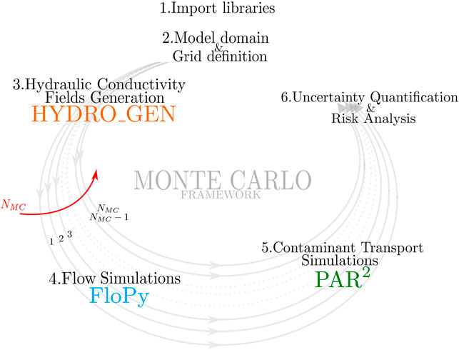
FIGURE 1. A schematic representation of VisU-HydRA. As a computational toolbox for groundwater contaminant transport and its uncertainty, VisU-HydRA integrates all necessary numerical software and post-processing codes in a single Jupyter Notebook. Each component (1-6) is executed by each code cell in the Jupyter Notebook in order. Colored are the names of the employed software, and NMC stands for the number of Monte Carlo realizations.
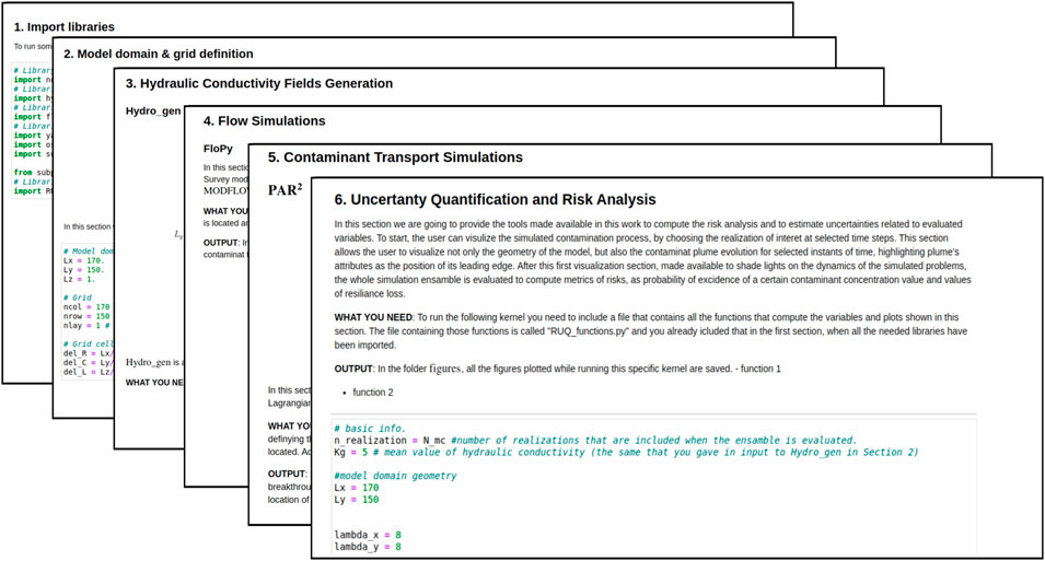
FIGURE 2. Examples of Jupyter Notebook code cells corresponding to the numbered processes (see Figure 1). Detailed descriptions are included in each cell so that users can easily reproduce the results of the tutorial presented in this study.
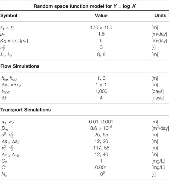
TABLE 1. Input parameters used in the proposed tutorial for hydraulic conductivity field generation and flow and transport simulations.
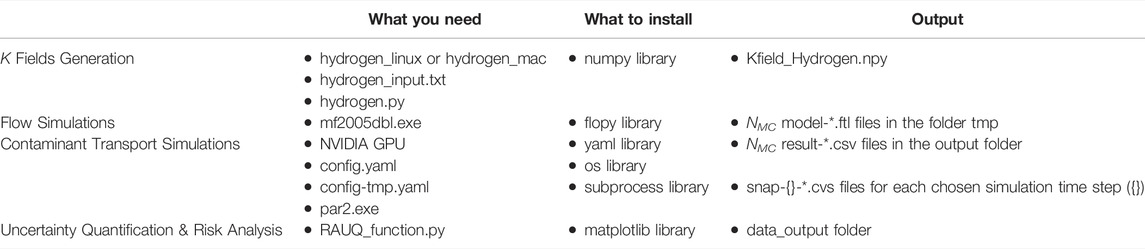
TABLE 2. A list of software, Python libraries, configuration files for each step and the corresponding output data. Users need to install and prepare them to run the tutorial that reproduces the data and the analysis shown in this work.
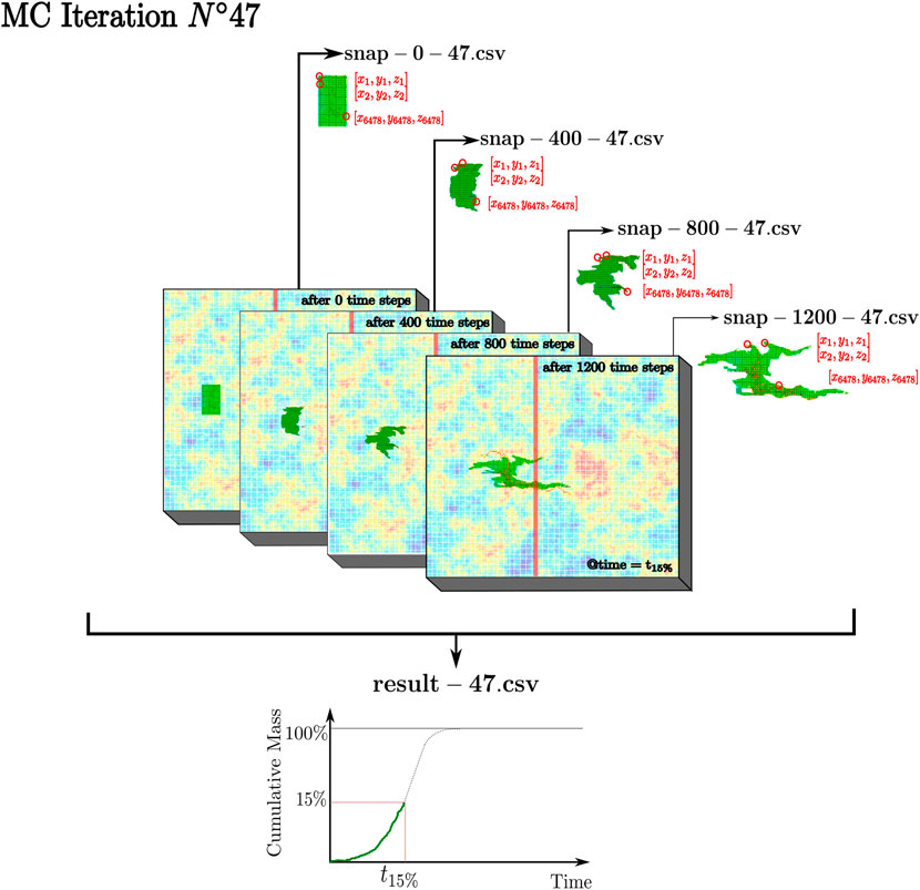
FIGURE 3. Schematic representation of the contaminant transport simulations code cell output. The image schematizes a possible output (depending on the declared parameters in the YAML file) of a randomly selected hydraulic conductivity field from the Monte Carlo ensemble (realization number 47). The model output for this specific hydraulic conductivity realization is given by “result-47.csv”. This file contains the data related to the contaminant’s cumulative breakthrough curve at the control plane (represented by the vertical red line). In addition, snapshot files are generated for 400 simulation time steps. For example, “snap-0-47.csv”, “snap-400-47.csv”, “snap-800-47.csv” and “snap-1200-47.csv” contain the position of each particle at time steps 0, 400, 800 and 1200. For visualization purposes, the position (x = [x, y, z]) of the 1st, 2nd and 6478th particles are highlighted by red circles.
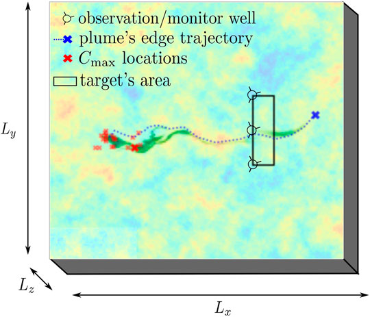
FIGURE 4. Schematic representation of the contaminant plume, in green, for a given random realization of the hydraulic conductivity field. The figure shows where observations wells (circles) are positioned over the target area (rectangle) and how the locations of the leading edge of the plume (blue cross) and of the maximum contaminant concentration (red cross), experienced at each time steps of the simulation, evolve in time. The trajectory of the leading edge of the plume follows the trajectory given by the dotted blue line. The location of the maximum concentration of the plume bounces from one location to another (see red crosses).
5 Application to Risk and Resilience
5.1 Probability of Concentration Exceedance and Resilience Loss Maps
We will now use VisU-HydRA to investigate the risks associated with an accidental benzene spill. For this hypothetical case study, we will consider a 2D simulation as previously described (therefore, x1 = x and x2 = y). All parameter values employed in the upcoming results are reported in Table 1. Benzene is a wildly used chemical for industrial solvents and for constituents of fossil fuels and is considered to be a major threat to groundwater resources and human health (Sivasankar et al., 2017). Benzene spills are typically associated with transportation and storage tank leakages. Due to its potential health risk (e.g., Logue and Fox, 1986), the State of California (United States) set the Maximum Contaminant Level, i.e. the highest level of a contaminant that is allowed in drinking water, to C* = 10–3 [mg/L] (Proctor et al., 2020). Note that benzene’s degradation in water is extremely slow (i.e., Sivasankar et al., 2017), and consequently, for the purpose of our illustration, we will assume transport to be non-reactive (see Eq. A2).
Figure 5 depicts the spatial map of the expected value of Ψ (Figure 5, top row), namely ⟨Ψ⟩, as well as its variance
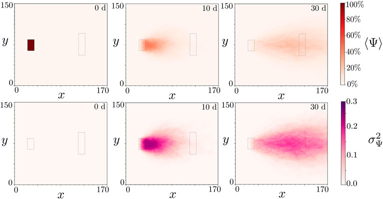
FIGURE 5. Maps of the probability of concentration exceedance (top), and its uncertainty (bottom) at different instant of time in the simulation (columns). Plots of the top row shows how ⟨Ψ⟩ [-] evolves in space respectively after 0, 10 and 30 days from the beginning of the contamination process. ⟨Ψ⟩ is expressed as a probability, as indicated by its values on the color bar on the right. The bottom row shows
Next, we analyze the loss of resilience of the aquifer system. Figure 6 shows the spatial map of first two statistical moments of RL, see Eq. 2. The results illustrated provide information regarding the locations where the expected resilience loss will be the largest (Figure 6A) and its corresponding uncertainty (Figure 6B). RL represents a measure of the amount of days necessary for the aquifer to recover up to a state where the risks associated with the contamination can be considered negligible.
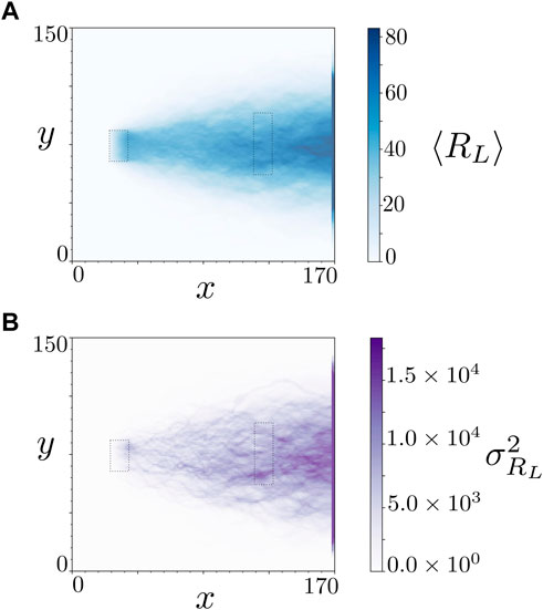
FIGURE 6. Maps of the average loss of resilience (A) in the model domain, and its variance values (B) throughout the whole simulation time. The plot on the top shows how ⟨RL⟩ [d] evolves in space, expressing the amount of days necessary for each point in the domain to recover up to a reliable status. The amount of days associated with the different shades of blue are indicated by the values on the color bar on the right of the top plot. The plot at the bottom shows the values of the variance of RL,
As expected, the values of ⟨RL⟩ increase with travel distance from the source location. This is explained by the increase of the macroscale dispersion as the plume moves downstream from the source. An increase in plume dispersion leads to the presence of long tails in the solute breakthrough curve. Therefore, the residence time for the plume while crossing a given location increases thus leading to an increase in the averaged resilience loss. As observed in Figure 6A, the maximum number of days necessary for the right boundary of the flow domain to recover is approximately 80. The results at the bottom of Figure 6 quantify the uncertainties related to the estimated resilience loss values. As shown in Figure 6B, larger uncertainty in RL is observed at large distances from the source. One possible explanation for this phenomenon may be due to the fact the contaminant plume has sampled more fluctuations of the velocity field (i.e. the plume travels through many correlation scales) thus leading to increased uncertainty in the solute breakthrough curves at those locations.
5.2 Impact of Contaminant Source Efficiency on Aquifer Reliability
The computational package VisU-HydRA can also be employed to improve our understanding on the impact of groundwater flow physics and decision making metrics such as RL. Here we illustrate how the hydraulics conditions within the contaminant source zone could be used as an indicator of RL. de Barros and Nowak (2010) introduced the source zone efficiency η
where Qsz is the volumetric flow rate [m3/days] crossing the contaminant source zone while Qb indicates the total background volumetric flow rate passing through the entire aquifer’s cross section. de Barros and Nowak (2010) showed that Eq. 4 controls the overall plume dispersion downstream from the source. Similar results are reported in Henri et al. (2016) in the context of risk analysis, where the authors showed that high water flux crossing the source zone leads to decrease in the magnitude of human health risk due to the presence of chlorinated solvents. Gueting and Englert (2013) also report experimental evidence regarding the importance of source zone hydraulics on transport behavior. Through the use of a Bayesian framework, Nowak et al. (2010) showed that characterizing the flow field surrounding the source zone could significantly reduce the uncertainty of transport observables.
Figure 7 shows the scatter plot of the maximum value of resilience loss RL experienced within the target area (
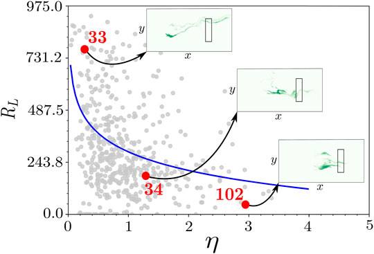
FIGURE 7. Maximum value of resilience loss (RL [d]) experienced within the target area versus contaminant source efficiency (η [-]) for all the Monte Carlo realizations. Data (gray dots) are fitted by a logarithmic curve, the blue line in the plot. The red dots highlight three Monte Carlo realizations, the 33rd, 34th and 102nd, in which the spatial configuration of the contaminant plume is investigated at a given time snapshot. The insets are connected, by a black arrow, to the simulated scenario. The black rectangles in the insets represent the environmentally sensitive target location.
6 Summary
In this work we provide VisU-HydRA, an open source, documented, computationally efficient toolbox to characterize specific features of the contaminant plume transport. The proposed package serves as a user-ready toolbox and allows to compute the uncertainty associated with metrics typically used in risk analysis. VisU-HydRA consists of a collection of rapid and open source software which have been assembled to deliver a rapid, reproducible and transparent modeling framework. Computational efficiency and rapidity are ensured by the usage of a GPU-accelerated solute transport simulator (Rizzo et al., 2019) and the automatized and solid structure of the iterative processes. Reproducibility and transparency are guaranteed by the open source coding language, the user-friendly interface of the Python code and the availability of a well documented and easy to follow tutorial made available on a web-based application.
In order to support the decision making process, the computational toolbox includes a visualization component that allows users to generate probability maps of aquifer resilience loss and risk hot spots. Furthermore, a GitHub repository was created and contains all the material reported to this work. The results reported are limited to a two dimensional application and the hydraulic conductivity field is the only source of uncertainty. As a consequence, the computational toolbox can be expanded to account for other sources of uncertainty as well as three dimensional models. In our work we opted to employ a two-dimensional “reference model” typically encountered in the stochastic hydrogeological community to study dispersion and mixing of solutes in heterogeneous aquifers. However, more realistic scenarios can be incorporated, such as the one reported in Fiori et al. (2019). We point out that the computational efficiency of the proposed toolbox could be improved by making use of other uncertainty quantification methodologies (as opposed to the classic Monte Carlo framework). For example, Olivier et al. (2020) presents an open-source, user-ready, Python package that includes several of the latest approaches for uncertainty estimation that are computationally efficient. The current contribution represents one step towards an integrated framework for analyzing groundwater contamination in risk assessment under uncertainty.
Data Availability Statement
The datasets presented in this study can be found in online repositories. The names of the repository/repositories and accession number(s) can be found below: https://github.com/mariamorvillo/VisU-HydRA.
Author Contributions
MM, JI and FdeB were responsible for the conceptualization of the work. MM and FdeB wrote, reviewed and edited the paper. MM and JI performed all the simulations, implemented the computer code and performed the computational analysis. FdeB supervised the work, provided assistance and constructive critical support. All authors contributed to the interpretation of the results, provided critical feedback and helped shape the research, analysis and manuscript.
Conflict of Interest
The authors declare that the research was conducted in the absence of any commercial or financial relationships that could be construed as a potential conflict of interest.
Publisher’s Note
All claims expressed in this article are solely those of the authors and do not necessarily represent those of their affiliated organizations, or those of the publisher, the editors and the reviewers. Any product that may be evaluated in this article, or claim that may be made by its manufacturer, is not guaranteed or endorsed by the publisher.
Acknowledgments
The authors acknowledge the constructive comments made by the reviewers and Dr. Anneli Guthke. The authors also acknowledge the support provided by NSF Grant Number 1654009.
Appendix A Flow and Transport Equations
For computational illustrations, we simulated a steady-state fully saturated incompressible flow in a spatially heterogeneous aquifer in absence of sink or sources. Flow is 2D, and in our computational 2D domain, x1 denotes the longitudinal dimension and x2 the transverse one. The steady flow field is governed by:
with h denoting the hydraulic head and K the hydraulic conductivity.
For all our simulations, we considered permeameter-like boundary conditions for the flow field. That is, no-flux boundary conditions in the transverse boundaries and constant heads, respectively hin and hout, are adopted in the inflow and outflow boundaries of the computational domain.
For the transport simulation we consider that instantaneous release of Benzene within a rectangular source zone of area
where C is the resident concentration, u is the velocity field, D is the local-scale dispersion tensor assumed to be anisotropic and defined as:
where Dm is the molecular diffusion, αL is the longitudinal (along x1) dispersivity and αT is the transverse (along x2) dispersivity.
References
Andričević, R., and Cvetković, V. (1996). Evaluation of Risk from Contaminants Migrating by Groundwater. Water Resour. Res. 32, 611–621.
Bakker, M., Post, V., Langevin, C. D., Hughes, J. D., White, J. T., Starn, J. J., et al. (2016). Scripting MODFLOW Model Development Using Python and Flopy. Groundwater 54, 733–739. doi:10.1111/gwat.12413
Ballio, F., and Guadagnini, A. (2004). Convergence Assessment of Numerical Monte Carlo Simulations in Groundwater Hydrology. Water Resour. Res. 40. doi:10.1029/2003wr002876
Bellin, A., and Rubin, Y. (1996). HYDRO_GEN: A Spatially Distributed Random Field Generator for Correlated Properties. Stoch. Hydrol. Hydraul. 10, 253–278. doi:10.1007/bf01581869
Boso, F., and Tartakovsky, D. M. (2016). The Method of Distributions for Dispersive Transport in Porous Media with Uncertain Hydraulic Properties. Water Resour. Res. 52, 4700–4712. doi:10.1002/2016wr018745
Cardiff, M., Liu, X., Kitanidis, P. K., Parker, J., and Kim, U. (2010). Cost Optimization of DNAPL Source and Plume Remediation under Uncertainty Using a Semi-analytic Model. J. Contam. Hydrology 113, 25–43. doi:10.1016/j.jconhyd.2009.11.004
Ciriello, V., and de Barros, F. P. J. (2020). Characterizing the Influence of Multiple Uncertainties on Predictions of Contaminant Discharge in Groundwater within a Lagrangian Stochastic Formulation. Water Resour. Res. 56, e2020WR027867. doi:10.1029/2020wr027867
Ciriello, V., Lauriola, I., Bonvicini, S., Cozzani, V., Di Federico, V., and Tartakovsky, D. M. (2017). Impact of Hydrogeological Uncertainty on Estimation of Environmental Risks Posed by Hydrocarbon Transportation Networks. Water Resour. Res. 53, 8686–8697. doi:10.1002/2017wr021368
Dabbish, L., Stuart, C., Tsay, J., and Herbsleb, J. (2012). “Social Coding in GitHub: Transparency and Collaboration in an Open Software Repository,” in Proceedings of the ACM 2012 conference on computer supported cooperative work, 1277–1286.
de Barros, F. P. J., Ezzedine, S., and Rubin, Y. (2012). Impact of Hydrogeological Data on Measures of Uncertainty, Site Characterization and Environmental Performance Metrics. Adv. Water Resour. 36, 51–63. doi:10.1016/j.advwatres.2011.05.004
de Barros, F. P. J., Fiori, A., Boso, F., and Bellin, A. (2015). A Theoretical Framework for Modeling Dilution Enhancement of Non-reactive Solutes in Heterogeneous Porous Media. J. Contam. Hydrology 175-176, 72–83. doi:10.1016/j.jconhyd.2015.01.004
de Barros, F. P. J., and Fiori, A. (2014). First-order Based Cumulative Distribution Function for Solute Concentration in Heterogeneous Aquifers: Theoretical Analysis and Implications for Human Health Risk Assessment. Water Resour. Res. 50, 4018–4037. doi:10.1002/2013wr015024
de Barros, F. P. J., and Fiori, A. (2021). On the Maximum Concentration of Contaminants in Natural Aquifers. Transp. Porous Med. 140, 273–290. doi:10.1007/s11242-021-01620-3
de Barros, F. P. J., and Nowak, W. (2010). On the Link between Contaminant Source Release Conditions and Plume Prediction Uncertainty. J. Contam. hydrology 116, 24–34. doi:10.1016/j.jconhyd.2010.05.004
de Barros, F. P. J., and Rubin, Y. (2008). A Risk-Driven Approach for Subsurface Site Characterization. Water Resour. Res. 44. doi:10.1029/2007wr006081
Dentz, M., Le Borgne, T., Englert, A., and Bijeljic, B. (2011). Mixing, Spreading and Reaction in Heterogeneous Media: A Brief Review. J. Contam. Hydrology 120-121, 1–17. doi:10.1016/j.jconhyd.2010.05.002
Dentz, M., and Tartakovsky, D. M. (2010). Probability Density Functions for Passive Scalars Dispersed in Random Velocity Fields. Geophys. Res. Lett. 37. doi:10.1029/2010gl045748
Fienen, M. N., and Bakker, M. (2016). HESS Opinions: Repeatable Research: what Hydrologists Can Learn from the Duke Cancer Research Scandal. Hydrol. Earth Syst. Sci. 20, 3739–3743. doi:10.5194/hess-20-3739-2016
Fienen, M. N., Corson‐Dosch, N. T., White, J. T., Leaf, A. T., and Hunt, R. J. (2022). Risk‐Based Wellhead Protection Decision Support: A Repeatable Workflow Approach. Groundwater 60, 71–86. doi:10.1111/gwat.13129
Fiori, A., Bellin, A., Cvetkovic, V., de Barros, F. P. J., and Dagan, G. (2015). Stochastic Modeling of Solute Transport in Aquifers: From Heterogeneity Characterization to Risk Analysis. Water Resour. Res. 51, 6622–6648. doi:10.1002/2015wr017388
Fiori, A., and Dagan, G. (2000). Concentration Fluctuations in Aquifer Transport: A Rigorous First-Order Solution and Applications. J. Contam. Hydrology 45, 139–163. doi:10.1016/s0169-7722(00)00123-6
Fiori, A., Zarlenga, A., Bellin, A., Cvetkovic, V., and Dagan, G. (2019). Groundwater Contaminant Transport: Prediction under Uncertainty, with Application to the MADE Transport Experiment. Front. Environ. Sci. 7, 79. doi:10.3389/fenvs.2019.00079
Gueting, N., and Englert, A. (2013). Hydraulic Conditions at the Source Zone and Their Impact on Plume Behavior. Hydrogeol. J. 21, 829–844. doi:10.1007/s10040-013-0962-7
Hammond, G. E., Lichtner, P. C., and Mills, R. T. (2014). Evaluating the Performance of Parallel Subsurface Simulators: An Illustrative Example with PFLOTRAN. Water Resour. Res. 50, 208–228. doi:10.1002/2012wr013483
Harbaugh, A. W. (2005). MODFLOW-2005, the US Geological Survey Modular Ground-Water Model: The Ground-Water Flow Process. Reston, VA, USA: US Department of the Interior, US Geological Survey Reston.
Henri, C. V., Fernàndez-Garcia, D., and de Barros, F. P. J. (2016). Assessing the Joint Impact of DNAPL Source-Zone Behavior and Degradation Products on the Probabilistic Characterization of Human Health Risk. Adv. Water Resour. 88, 124–138. doi:10.1016/j.advwatres.2015.12.012
Im, J., Rizzo, C. B., de Barros, F. P. J., and Masri, S. F. (2021). Application of Genetic Programming for Model-free Identification of Nonlinear Multi-Physics Systems. Nonlinear Dyn. 104, 1781–1800. doi:10.1007/s11071-021-06335-0
Im, J., Rizzo, C. B., and de Barros, F. P. J. (2020). Resilience of Groundwater Systems in the Presence of Bisphenol A under Uncertainty. Sci. Total Environ. 727, 138363. doi:10.1016/j.scitotenv.2020.138363
Kapoor, V., and Kitanidis, P. K. (1998). Concentration Fluctuations and Dilution in Aquifers. Water Resour. Res. 34, 1181–1193. doi:10.1029/97wr03608
Kitanidis, P. K. (1997). Introduction to Geostatistics: Applications in Hydrogeology. Cambridge: Cambridge University Press.
Li, S.-G., and Liu, Q. (2006). Interactive Ground Water (IGW). Environ. Model. Softw. 21, 417–418. doi:10.1016/j.envsoft.2005.05.010
Logue, J. N., and Fox, J. M. (1986). Residential Health Study of Families Living Near the Drake Chemical Superfund Site in Lock Haven, Pennsylvania. Archives Environ. Health Int. J. 41, 222–228. doi:10.1080/00039896.1986.9938337
Maxwell, R. M., Carle, S. F., and Tompson, A. F. B. (2008). Contamination, Risk, and Heterogeneity: on the Effectiveness of Aquifer Remediation. Environ. Geol. 54, 1771–1786. doi:10.1007/s00254-007-0955-8
Maxwell, R. M., Condon, L. E., and Kollet, S. J. (2015). A High-Resolution Simulation of Groundwater and Surface Water over Most of the Continental US with the Integrated Hydrologic Model ParFlow V3. Geosci. Model. Dev. 8, 923–937. doi:10.5194/gmd-8-923-2015
Meyer, D. W., Tchelepi, H. A., and Jenny, P. (2013). A Fast Simulation Method for Uncertainty Quantification of Subsurface Flow and Transport. Water Resour. Res. 49, 2359–2379. doi:10.1002/wrcr.20240
Mood, A. M., Graybill, F. A., and Boes, C. D. (1974). Introduction to the Theory of Statistics. International Student Edition. New York, NY, USA: McGraw-Hill.
Neuman, S. P., and Tartakovsky, D. M. (2009). Perspective on Theories of Non-fickian Transport in Heterogeneous Media. Adv. Water Resour. 32, 670–680. doi:10.1016/j.advwatres.2008.08.005
Nowak, W., De Barros, F. P. J., and Rubin, Y. (2010). Bayesian geostatistical design: Task‐driven optimal site investigation when the geostatistical model is uncertain. , 46(3). Water Resour. Res. 46(3).
Oladyshkin, S., and Nowak, W. (2012). Data-driven Uncertainty Quantification Using the Arbitrary Polynomial Chaos Expansion. Reliab. Eng. Syst. Saf. 106, 179–190. doi:10.1016/j.ress.2012.05.002
Olivier, A., Giovanis, D. G., Aakash, B. S., Chauhan, M., Vandanapu, L., and Shields, M. D. (2020). Uqpy: A General Purpose python Package and Development Environment for Uncertainty Quantification. J. Comput. Sci. 47, 101204. doi:10.1016/j.jocs.2020.101204
Peñuela, A., Hutton, C., and Pianosi, F. (2021). An Open-Source Package with Interactive Jupyter Notebooks to Enhance the Accessibility of Reservoir Operations Simulation and Optimisation. Environ. Model. Softw. 145, 105188. doi:10.1016/j.envsoft.2021.105188
Proctor, C. R., Lee, J., Yu, D., Shah, A. D., and Whelton, A. J. (2020). Wildfire Caused Widespread Drinking Water Distribution Network Contamination. AWWA Water Sci. 2, e1183. doi:10.1002/aws2.1183
Rizzo, C. B., Nakano, A., and de Barros, F. P. J. (2019). PAR2: Parallel Random Walk Particle Tracking Method for Solute Transport in Porous Media. Comput. Phys. Commun. 239, 265–271. doi:10.1016/j.cpc.2019.01.013
Siirila, E. R., Navarre-Sitchler, A. K., Maxwell, R. M., and McCray, J. E. (2012). A Quantitative Methodology to Assess the Risks to Human Health from CO2 Leakage into Groundwater. Adv. Water Resour. 36, 146–164. doi:10.1016/j.advwatres.2010.11.005
Sivasankar, V., Senthil kumar, M., and Gopalakrishna, G. (2017). Quantification of Benzene in Groundwater Sources and Risk Analysis in a Popular South Indian Pilgrimage City–A GIS Based Approach. Arabian J. Chem. 10, S2523–S2533. doi:10.1016/j.arabjc.2013.09.022
vanRossum, G. (1995). Python Reference Manual. Blacksburg, VA, USA: Department of Computer Science [CS].
White, J. T., Foster, L. K., Fienen, M. N., Knowling, M. J., Hemmings, B., and Winterle, J. R. (2020). Toward Reproducible Environmental Modeling for Decision Support: a Worked Example. Front. Earth Sci. 8, 50. doi:10.3389/feart.2020.00050
Woodruff, M. J., Reed, P. M., and Simpson, T. W. (2013). Many Objective Visual Analytics: Rethinking the Design of Complex Engineered Systems. Struct. Multidisc Optim. 48, 201–219. doi:10.1007/s00158-013-0891-z
Ye, Y., Chiogna, G., Cirpka, O. A., Grathwohl, P., and Rolle, M. (2015). Enhancement of Plume Dilution in Two‐dimensional and Three‐dimensional Porous Media by Flow Focusing in High‐permeability Inclusions. Water Resour. Res. 51, 5582–5602. doi:10.1002/2015wr016962
Zhang, D., Shi, L., Chang, H., and Yang, J. (2010). A Comparative Study of Numerical Approaches to Risk Assessment of Contaminant Transport. Stoch. Environ. Res. Risk Assess. 24, 971–984. doi:10.1007/s00477-010-0400-5
Keywords: uncertainty quantification (UQ), stochastic hydrogeology, reproducible, decision making, probabilistic risk analysis
Citation: Morvillo M, Im J and de Barros FPJ (2022) VisU-HydRA: A Computational Toolbox for Groundwater Contaminant Transport to Support Risk-Based Decision Making. Front. Earth Sci. 10:916198. doi: 10.3389/feart.2022.916198
Received: 08 April 2022; Accepted: 23 May 2022;
Published: 14 June 2022.
Edited by:
Anneli Guthke, University of Stuttgart, GermanyReviewed by:
Md Nazmul Azim Beg, Tulane University, United StatesMariaines Di Dato, Helmholtz-Zentrum für Umweltforschung UFZ, Germany
Copyright © 2022 Morvillo, Im and de Barros. This is an open-access article distributed under the terms of the Creative Commons Attribution License (CC BY). The use, distribution or reproduction in other forums is permitted, provided the original author(s) and the copyright owner(s) are credited and that the original publication in this journal is cited, in accordance with accepted academic practice. No use, distribution or reproduction is permitted which does not comply with these terms.
*Correspondence: Maria Morvillo, bW9ydmlsbG9AdXNjLmVkdQ==