 M. Massa
 S. Lovati
 R. Puglia
 G. Brunelli
 F. Pacor
95% of researchers rate our articles as excellent or good
Learn more about the work of our research integrity team to safeguard the quality of each article we publish.
Find out more
ORIGINAL RESEARCH article
Front. Earth Sci. , 14 June 2022
Sec. Geohazards and Georisks
Volume 10 - 2022 | https://doi.org/10.3389/feart.2022.915083
This article is part of the Research Topic New Challenges for Seismic Risk Mitigation in Urban Areas View all 11 articles
In this paper, we present the work carried out to characterize the spatial variability of seismic site response related to local soil conditions in the city of Milan and its surroundings, an area with ∼3 million inhabitants and a high density of industrial facilities. The area is located at the northwestern end of the Po Plain, a large and deep sedimentary basin in northern Italy. An urban-scale seismo-stratigraphic model is developed based on new passive and active seismic data, supported by the available geological data and stratigraphic information from shallow and deep vertical wells. In particular, 33 single-station and 4 ambient-vibration array measurements are acquired, together with 4 active multichannel analyses of surface waves (MAWS). To estimate the resonant frequencies of the sediments, the horizontal to vertical spectral ratio technique (HVSR) is applied to the ambient-vibration recordings, whereas to determine the Rayleigh-wave dispersion curves from the passive array, the data are analysed using the conventional frequency-wavenumber, the modified spatial autocorrelation and the extended spatial autocorrelation (ESAC) techniques. The array data are used to determine the local shear wave velocity profiles, VS, via joint inversion of the Rayleigh-wave dispersion and ellipticity curves deduced from the HVSR. The results from HVSR show three main bands of amplified frequencies, the first in the range 0.17–0.23 Hz, the second from 0.45 to 0.65 Hz and the third from 3 to 8 Hz. A decreasing trend of the main peaks is observed from the northern to the southern part of the city, allowing us to hypothesize a progressive deepening of the relative regional chrono-stratigraphic unconformities. The passive ambient noise array and MASW highlight the dispersion of the fundamental mode of the Rayleigh-wave in the range 0.4–30 Hz, enabling to obtain detailed Vs. profiles with depth down to about 1.8 km. The seismo-stratigraphic model is used as input for 1D numerical modelling assuming linear soil conditions. The theoretical 1D transfer functions are compared to the HVSR curves evaluated from both ambient noise signals and earthquake waveforms recorded by the IV. MILN station in the last 10 years.
It is widely recognized that a significant proportion of the variability of earthquake ground motion is related to local geological conditions, which can modify the ground-motion amplitude, duration, and frequency. In alluvial basins (or valleys), layers can cause resonance of vertically propagating shear waves at specific frequencies and/or trap surface waves generated locally at the edges of the basin (e.g., Hanks, 1975; Hisada et al., 1993; Bielak et al., 1999; Sato et al., 1999; Joyner, 2000; Kagawa et al., 2004; Somerville et al., 2004; D’Amico et al., 2006; D’Amico et al., 2008; De Ferrari et al., 2010; Ronald Abraham et al., 2015).
In this framework and in particular for urban planning (e.g. Ansal et al., 2009; Ansal et al., 2010, Crespellani 2014, Celikbilek and Sapmaz 2016, Aversa and Crespellani 2016, etc.), the seismic site effect estimation plays a crucial role in earthquake risk reduction.
The importance of site characterization of urban or metropolitan areas is recognized worldwide, with several studies performed in New York (Stephenson et al., 2009), Taipei (Wang, 2008), Perth (Liang et al., 2009), Seoul (Sun et al., 2014; Kim et al., 2017), Beijing (Liu et al., 2014), Vancouver (Molnar et al., 2020), San Josè, Costa Rica (Moya et al., 2000), Istanbul (Picozzi et al., 2009; Ansal et al., 2010), Memphis (Schneider et al., 2001), Bucharest (Ritter et al., 2005), among others.
Similar studies in Italy are performed for other cities like Matera (Tragni et al., 2021), Rome (Marcucci et al., 2019), and Firenze (D’Amico et al., 2008), as well as small villages like Mirandola (Tarabusi and Caputo, 2017) and Cavezzo (Lai et al., 2020), both located in the Po plain and strongly struck by the 2012 Emilia seismic sequence (Luzi et al., 2013). Worth mentioning is the intensive studies that have been performed after the 2016–2017 Central Italy seismic sequence (Michele et al., 2016) to obtain detailed microzonation maps in the 138 most damaged municipalities (Hailemikael et al., 2020).
In this paper, we focus on the city of Milan, with an area of about 1.570 km2 and a population of more than 3 million (http://www.istat.it). Milan and its hinterlands represent the area with the highest density of industrial plants, service industries, skyscrapers and high-speed railways in Italy (http://www.istat.it). In particular, Milan is the Italian city that has grown more vertically through the construction of skyscrapers, at present with maximum height of ∼230 m and 50 stories (https://en.wikipedia.org/wiki/List_of_tallest_buildings_in_Milan). Recently, a couple of 5s seismometers, with reserved data, is installed at the floors −3 (i.e., −15 m from surface) and 37 (height ∼140 m), respectively, of the skyscraper Lombardia-building (https://en.wikipedia.org/wiki/Palazzo_Lombardia), allowing us to preliminary recognize a natural periods of vibration of ∼3.2 s.
The MMA (northern Italy, Figure 1, panel A) is located in the northwestern part of the Po Plain, one of the largest alluvial basins worldwide. The Po alluvial basin covers an area of about 50.000 km2, with alluvial deposits that can reach a depth of several kilometers and that directly overlie the deep Miocene geological bedrock (Pieri and Groppi, 1981; Regione Lombardia, Eni Divisione Agip, 2002).
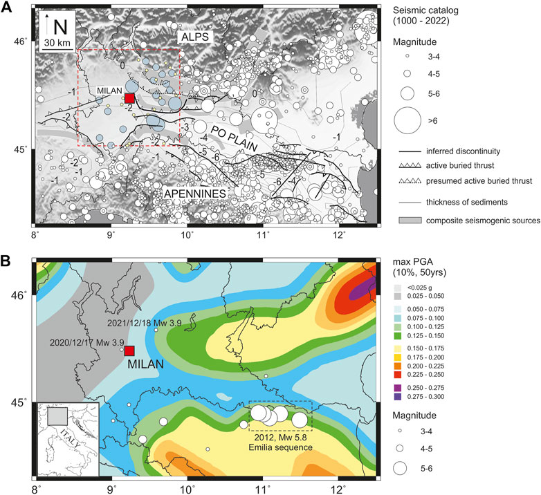
FIGURE 1. Panel (A) simplified structural sketch of the Po plain (from Pieri and Groppi, 1981; Bigi et al., 1990). The red square indicates the urban area of Milan. White circles indicate the seismicity from yrs. 1000 to 2022. Dark gray and yellow circles drawn in the red inset indicate the recent (after 1 January 1985, http://terremoti.ingv.it/) and the historical seismicity (yrs. 1000–1985, https://emidius.mi.ingv.it/CPTI15-DBMI15/; Rovida et al., 2020), respectively, occurred in an area of 100 km2 around the MMA. The composite seismogenic sources are derived from DISS (Database of Individual Seismogenis Sources, http://diss.ingv.it). Panel (B) Seismic hazard maps of Italy (MPS Working Group, 2004; Stucchi et al., 2011), in terms of peak ground acceleration (PGA) with 10% possibility of exceedance in 50 years (i.e., a return period of 475 years), referred to the rigid soils (i.e., Vs. > 800 m/s; NTC 2018). White circles indicate the epicenters of the earthquakes used for the HVSR analyses (see also Table 1).
The bottom panel of Figure 1 (panel B) shows the reference Italian seismic hazard map of Italy in terms of peak ground acceleration for rock-site conditions with 10% probability of exceedance in 50 years (MPS Working Group, 2004; Stucchi et al., 2011): despite the low-to-medium seismic hazard of the area, the exposure level of the city, the local geological condition (Figure 2) and the proximity with active buried seismogenic structure (Figure 1, panel A) make the MMA a medium to high seismic risk zone.
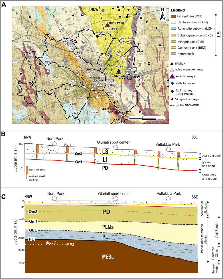
FIGURE 2. Panel (A) 1:10000 Geological map from the 118 Milan sheet (ISPRA et al., 2016). Po synthem (POI, Upper Pleistocene-Holocene), Cantù synthem (LCN, Upper Pleistocene), Ronchetto delle Rane subsynthem (LCN4, Upper Pleistocene), Bulgarograsso unit (BXE, Middle-Upper Pleistocene), Minoprio Unit (BMI, Middle-Upper Pleistocene) and Guanzate unit (BEZ, Middle-Upper Pleistocene) are the stratigraphic units characterizing the MMA (ISPRA et al., 2016). The dotted black line indicates the NNW-SSE geological section showed in panel (B). Panel (B) geological section from North Park (NNW) to Vettabbia park (SSE), with thickness of about 200 m. Yellow line represents the Qc3 Unconformity from GeoMol Team, 2015 (or Y-Surface from Scardia et al., 2012), while red line represents the Qc1 Unconformity from GeoMol Team, 2015 (or R-Surface from Muttoni et al., 2003). LS and LI indicate the upper and lower Padano supersynthem, while PD indicates the Padano supersynthem (ISPRA et al., 2016). Panel (C) geological section from North Park (NNW) to Vettabbia park (SSE), with thickness of about 1800 m. MESa (Burdigalian-Tortonian), MESb (Messinian), PL (early-middle Pliocene) and PLMa (Middle lower Pleistocene) indicate the stratigraphic units as recognized by GeoMol project (2015), while PL (base of Pliocene, 5,3 Myrs), GEL (base of Pleistocene, 2,6 Myrs), Qm1 (1,5 Myrs) and Qm2 (1,25 Myrs) represent the related unconformities. Dotted lines indicate the deduced depths on the basis of the ViDEPI project (2009) deep wells.
The studied area is, in general, characterized by a low rate of annual seismicity (Figure 1, panel A). In particular, in the last 40 years no local earthquakes with magnitude >4.5 have occurred. However, the area has often undergone ground motion over the long-period, namely in the case of distant earthquakes with higher magnitude, such as the 2012 Emilia, Mw 5.8, seismic sequence (Luzi et al., 2013).
The importance of the long-period (>1 s) component of seismic ground motion has been recognized worldwide during some strong earthquakes (e.g., 1985, Mw 8.1, Michoacán, Furumura and Kennett, 1998; Furumura and Kennett, 1999, Mw 7.1, Hector Mine, Grazier et al., 2002, Mw 7.9, Denali, Ratchkovski et al., 2003, Mw 8.0, Tokachi-Oki, Miyazaki et al., 2004). Significant damage to long-period structures at large hypocentral distances, as well as prolonged duration of seismic ground motion, has prompted seismologists to focus in understanding the seismic wave propagation and amplification effects in deep sedimentary basins. The Mexico City records of the 1985 Michoacan earthquake lead to far source long-period ground motions being known around the world, with long-period components between 2 and 4 s (Beck and Hall, 1986). Before the 1985 Michoacan earthquake, Japanese seismologists observed far-source long-period ground motion in the Niigata basin, during the 1964 Niigata, 1968 Tokachi-oki, and 1983 Japan Sea earthquakes (Koketsu and Miyake, 2008). Subsequently, the 2003 Tokachi-oki earthquake provided the southern coast of Hokkaido in Japan, with one of the most significant examples (Koketsu et al., 2005; Hatayama, 2008) of far-source long-period ground motion, with dominant amplitudes in the range 7–8 s and displacements of a few meters (Koketsu and Miyake, 2008).
Long-period ground motion amplification is a significant issue in the Po Plain. In this area, long-period resonance phenomena have been well-documented by many studies (e.g., Priolo et al., 2012; Luzi et al., 2013; Martelli and Romani, 2013; Massa and Augliera, 2013; Milana et al., 2013; Paolucci et al., 2015; Laurenzano et al., 2017; Mascandola et al., 2017; Tarabusi and Caputo, 2017). However, most of these are performed in the epicentral area of the 2012 Emilia seismic sequence (e.g., Luzi et al., 2013), during which significant ground-motion amplifications and increased duration are observed. A recent study by Mascandola et al. (2019) widely mapped 1–3 s long-period resonance phenomena in the Po Plain, through extensive ambient-vibration measurements performed in the basin.
This study attempts to investigate the influence of the shallow to deep (down ∼1.8 km) alluvial deposits for the metropolitan area of Milan, where amplification effects in the frequency range 0.2–8 Hz are observed. Milan has the disadvantage of having few earthquake recordings due to the relatively low seismicity and distant reference sites in the Alps or in the Apennine Mountains (Figure 1, panel A). These features prevent applying the standard spectral ratio approach (SSR, Bocherdt, 1970) to compute the empirical soil amplification functions and lead to adopting techniques based on numerical modelling, which are more accurate the more detailed the seismo-stratigraphic model is.
Therefore, in this study a detailed seismo-stratigraphic model obtained from the analysis of existing geological and stratigraphic data (e.g., Regione Lombardia, Eni Divisione Agip, 2002; Muttoni et al., 2003; De Franco et al., 2009; ViDEPI project, 2009; Scardia et al., 2012; GeoMol Team, 2015; ISPRA et al., 2016) and newly acquired geophysical data is proposed.
Different active and passive seismic measurements are carried out to characterize the subsoil. The passive analyses represent the main part of the study, consisting of 33 single-station and 4 array measurements of ambient noise (Figure 2, panel A). The single-station measurements allowed defining the resonance frequency of the site through the Nakamura (1989) horizontal-to-vertical spectral ratio (HVSR) method. The microtremor arrays, performed in correspondence of three selected sites (i.e., North Park, Giuriati sports center, Vettabbia park) located along the alignment reported in Figure 2 (panel A), enabled assessing vs. profiles down to depths of about ∼1.8 km.
The active measurements consisted of 4 Multichannel Analyses of Surface Waves (MASW, Park et al., 1999) at North and Vettabbia public parks (Figure 2, panel A) which are useful to define the soil categories, according to the Italian (Nuove Norme Tecniche per le Costruzioni, NTC, 2018) and the European (Eurocode 8, CEN 2004) seismic codes for buildings. Soil categories are defined according to the values of the average seismic shear-wave velocity from the surface to a depth of 30 m (VS,30).
The results obtained from ambient noise HVSR are compared to the HVSR curves considering 17 earthquakes with magnitude from 3.7 to 5.8 recorded by the IV. MILN station (Figure 2, panel B) in the last 10 years (Table 1).
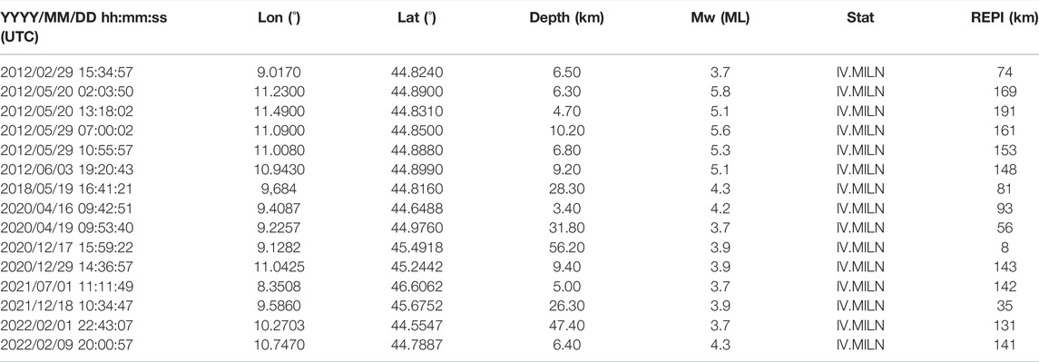
TABLE 1. Earthquakes with magnitude ≥3.7 recorded at station IV.MILN in the last 10 years and used for the HVSR analyses. The epicentres are depicted in panel B) of Figure 1. In bold are indicated magnitude values > 5.
The Vs profiles are finally validated through 1D numerical models performed assuming a linear elastic behaviour of the soil using the SHAKE91 code (Idriss and Sun, 1993).
In the last 30 years, thousands of small-energy seismic events (∼200/year, Figure 1, panel A, http://terremoti.ingv.it/) have occurred in the Po Plain. Except of the 20 May 2012, Mw 5.8, Emilia seismic sequence (Luzi et al., 2013), with epicenters located 170 km southeast of Milan, the western part of the Po Plain area underwent a few moderate events, with magnitude between 4.5 and 5.5, such as the 14th August 2000, Mw 4.8, Asti the 3rd April 2003, Mw 4.8, Novi Ligure, the 14th September 2003, Mw 5.2, Monghidoro, the 24th November 2004, Mw 5.2, Salò and the 23rd December 2008, Mw 5.4, Parma events (http://terremoti.ingv.it). These moderate earthquakes did not cause losses of human life, but had negative economic consequences amounting to hundreds of millions of Euros (e.g., damage to buildings, schools, churches, industrial facilities etc.) highlighting the high degree of exposure of the region.
Focusing on MMA, the most powerful events recorded in the last decades occurred on 17th December 2020 (Mw 3.9 at epicentral distance of 5 km, http://terremoti.ingv.it) and on 18th December 2021 (Mw 3.9 at epicentral distance of 35 km, http://terremoti.ingv.it). In particular, in the past 10 years, the station IV. MILN (http://terremoti.ingv.it/instruments/station/MILN), now installed at INGV Milan department, recorded 17 seismic events in the magnitude (Mw) range 3.7–5.8, with epicentral distances up to 200 km (Table 1). Considering the historical seismicity (Rovida et al., 2020; https://emidius.mi.ingv.it/CPTI15-DBMI15/), the more significant earthquakes that struck the MMA occurred along the buried thrust systems reported in Figure 1 (panel A). The main seismogenic sources of the area (Figure 1, panel A) are derived from the Database of Individual Seismogenis Sources (DISS, http://diss.ingv.it). Considering 100 km2 around MMA, (Figure 1, panel A), the main historical events occurred on 26th November 1369 (Monza, Mw 5.33), on 12th May 1802 (Valle dell’Oglio, Mw 5.60), on 7th April 1786 (Po Plain, Mw 5.22) and on 15th May 1951 (Lodigiano, Mw 5.17). The highest macroseismic intensity (I = 7, https://emidius.mi.ingv.it/CPTI15-DBMI15/) for the area is associated to the 3rd January 1117, Mw 6.52, Verona earthquake, occurred ∼140 km, South-East of MMA.
Figure 3 shows the ground motion values recorded by the IV. MILN station in terms of peak ground acceleration (PGA), peak ground velocity (PGV) and response spectral (Sa) ordinates at period (T) of 3.0 s. The highest values of shaking in terms of acceleration is recorded on the 18th December 2021, Mw 3.9, Dalmine event (2021/12/18 10:34:47 UTC, http://terremoti.ingv.it) with maxima horizontal and vertical PGAs of 36 gal and 13 gal, respectively. PGAs between 5 gal and 10 gal, are recorded during the 17th December 2020, Mw 3.9, Pero event (2020/12/17 15:59:22 UTC, http://terremoti.ingv.it) and the 20th and 29th May 2012 Emilia main events (2012/05/20 02:03:52 UTC, Mw 5.8 and 2012/05/29 07:00:03 UTC, Mw 5.6, http://terremoti.ingv.it). This sequence produced seismic motion characterized by the dominance of surface waves (Love and Rayleigh waves) with amplitude higher than S-phases and by the arrival of a quasi-monochromatic wave train centered at 0.2 Hz. This phenomenon, described in Luzi et al. (2013) is more evident in the central and eastern sectors of the Po Plain, even if it is also observed at IV. MILN station in the case of the 20 May 2012, Mw 5.8, Emilia mainshock.
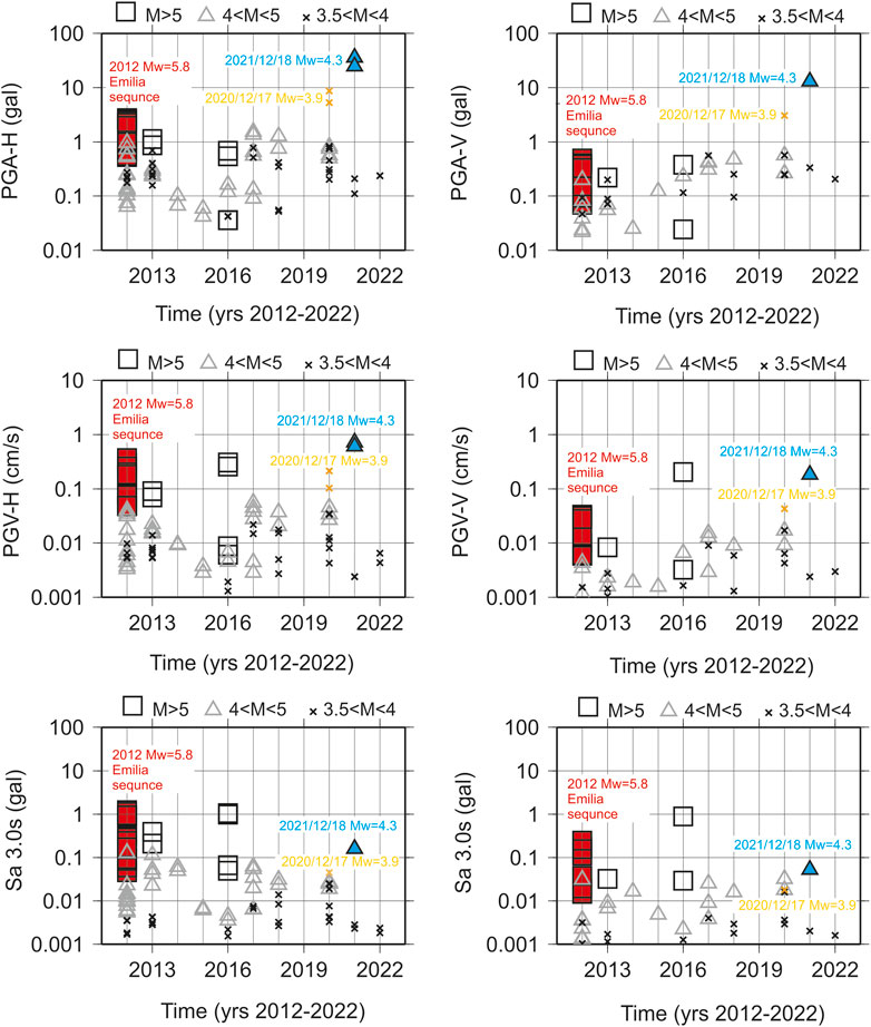
FIGURE 3. Peak Ground Acceleration (PGA), Velocity (PGV) and response spectral ordinates at period of 3.0 s for all events of magnitude ≥3.5 recorded at IV. MILN station from 1st January 2012. Left and right side indicate the horizontal and the vertical ground motion values, respectively.
The municipality of Milan (Figure 1, panel A) is located in the north-western sector of the Po Plain, a large and deep sedimentary basin between the south-verging thrust system of the Alps and the north-verging thrust system of the Apennines (Pieri and Groppi, 1981; Bigi et al., 1990); Figure 1 (panel A) also shows the expected maximum thickness of the Po plain sediments, represented by light grey contour lines. The Plio-Quaternary deposits of the Po Plain, overlie, in discordance, the geologic bedrock composed of deep-sea turbiditic deposits, which are deformed by compressive tectonic phases that lasted until the Upper Miocene along the piedmont edge of the Southern Alps. Since the Messinian, the tectonic phases of alpine structures stopped and the northern Apennines migrated towards NE. Since that time, the deposition and the geometries of the Po plain have been constrained by rapid uplift and forward movements of Apennine system, and to very long periods of isostatic subsidence of the basin.
From the available geological and geophysical information, a subsoil model with depth down to ∼1.8 km is built up along a NNW-SSE section, that crosses the three sites selected for the geophysical surveys (i.e., North Park, Giuriati sports center and Vettabbia park, see Figure 2, panel A).
In particular, we made use of:
- the 1:10.000 sheet 118 geological map (ISPRA et al., 2016);
- 5 selected water wells down to 120 m in depth (blue circles, Figure 2, panel A) available at https://www.geoportale.regione.lombardia.it/;
- one core drilling down to 100 m in depth (brown circle, Figure 2, panel A) performed in the framework of the Carg Project (ISPRA et al., 2016);
- the deep wells of ViDEPI project (2009) surrounding the metropolitan area of Milan (black circles in Figure 2, panel A);
- the stratigraphic units from Carg (ISPRA et al., 2016) and GeoMol Team (2015) projects;
- the isobaths published by ISPRA et al. (2016), in the framework of the Carg project (https://www.isprambiente.gov.it/Media/carg/118_MILANO_SOTTO/Foglio.html);
- the North South high-resolution reflection seismic profile acquired in the western area of Milan by De Franco et al. (2009).
The geological map reported in Figure 2 (panel A) show with different colours all the outcropping units of the 118-Milano geological sheet that belong to the Upper Pleistocene-Holocene continental succession. From a lithological point of view, these surface units are characterized by coarse and medium gravels, with subordinate levels of medium and coarse sands, and belong to the Supersintema Lombardo Superiore (LS).
The stratigraphy units from the top to the bottom are (Figure 2, panels B,C):
(1) LS unit (Supersintema Lombardo Superiore, Upper Pleistocene-Holocene; ISPRA et al., 2016, Figure 2, panel B) or group or aquifer-A (Regione Lombardia, Eni Divisione Agip, 2002) is made of clast-supported gravel, medium-coarse gravel and sparse pebbles (Scardia et al., 2012). LS is marked at the base by the Qc3 (Figure 2, panel B) regional chronostratigraphic Unconformity (0,45 My, GeoMol Team, 2015) or Y-surface (Scardia et al., 2012) that defines a regional change in fluvial depositional style (i.e., proximal braidplain according to Scardia et al., 2012), suggesting the occurrence of important erosional processes. All the outcropping units of the 118-Milano geological sheet (Figure 2, panel A) are sub-units of LS. LS unit has an average thickness of 50 m (Figure 2, panel b and Table 2);
(2) LI unit (Supersintema Lombardo Inferiore, Upper Pleistocene; ISPRA et al., 2016, Figure 2, panel B) or group acquifer-B (Regione Lombardia, Eni Divisione Agip, 2002) is an alternation of medium to coarse grained sand, gravel and subordinate silt, interpreted as a distal braidplain with wandering fluvial channels (Scardia et al., 2012). At the bottom, LI is marked by Qc1 (Figure 2, panel B), a regional chronostratigraphic Unconformity (0,87 My, GeoMol Team, 2015) or R-surface (Muttoni et al., 2003), correlated to the onset of major Pleistocene glaciations in the Alps. The average thickness of LI unit ranges from about 50 to 75 m moving NNW-SSE (Figure 2, panel B and Table 2);
(3) PD unit (Padano Supersynthem, Middle lower Pleistocene; ISPRA et al., 2016, Figure 2, panel C) is made of marine coastal and platform deposits (sand, with some clay layers) at the base, that evolve upwards to delta, delta-conoid and lagoon sediments (fine and very fine sand, mud, clay with some organic material, locally gravel) and to completely continental deposits (meandering river depositional system in alluvial plain, Scardia et al., 2012).
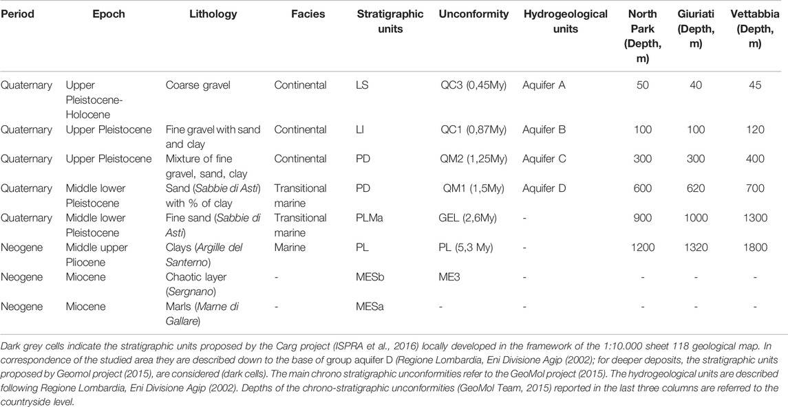
TABLE 2. Subsoil models at North park, Giuriati sports center and Vettabbia park.
In between, the transition from marine to continental environment is defined by the regional 1,25 My unconformity called Qm2 (GeoMol Team, 2015, Figure 2, panel C), corresponding to the bottom of group acquifer-C (Regione Lombardia, Eni Divisione Agip, 2002); at the base, PD is marked by the 1,5 My unconformity called Qm1 (GeoMol Team, 2015) that corresponds to the base of group acquifer-D (Regione Lombardia, Eni Divisione Agip, 2002). The average thickness of the PD unit ranges from about 500 to 600 m moving NNW-SSE (Figure 2, panel c and table 2);
(4) PLMa unit (Middle lower Pleistocene, Geomol Team, 2015, Figure 2, panel C) is made of sand deposits with some clay levels and thin gravel layers saturated with salty water (i.e., “Sabbie di Asti” formation, Regione Lombardia, ENI Divisione Agip 2002). At the bottom, PLMa unit is marked by the 2,6 My GELasian Unconformity (GeoMol Team, 2015). The average thickness of the PLMa unit range from about 300 to 600 m moving NNW-SSE (Figure 2, panel C and Table 2);
(5) PL unit (early-middle Pliocene, Geomol Team, 2015, Figure 2, panel C) is made of mud and clay deposits (i.e., “Argille del Santerno” formation, Dondi et al., 1982). At the base, the PL unit is marked by the 5,3 My intra Zanclean Unconformity called PL (“base of Pliocene”, GeoMol Team, 2015). The average thickness of the PL unit ranges from about 300 to 500 m moving NNW-SSE (Figure 2, panel C and Table 2);
(6) MESa unit (Burdigalian-Tortonian, GeoMol Team, 2015, Figure 2, panel C) is characterized by the “Marne di Gallare” formation (Rizzini and Dondi, 1978), that represents the geological bedrock of the area. In between, the formation is broken off at the top by the ME3 intra Messinian Unconformity (GeoMol Team, 2015, Figure 2, panel C), that marks the transition to the Messinian “Ghiaie del Sergnano” formation (chaotic gravel and sand, cemented levels, marls and sandstone, ViDEPI project 2009), that represents the potential reservoir between the Miocenic marls and the caprock of “Argille del Santerno,” a target of oil exploration.
The subsoil schemes describing the geological cross section of Figure 2 (panels B, C) are presented in Table 2. In particular, the depths of the Qc3, Qc1 and PL unconformities (Geomol project, 2015) are well-constrained by the isobaths published in the framework of the Carg project (https://www.isprambiente.gov.it/Media/carg/118_MILANO_SOTTO/Foglio.html, ISPRA et al., 2016), while the depths of the QM2, QM1, GEL unconformities (Geomol project, 2015) are deduced on the basis of the stratigraphy of ViDEPI project (2009).
From March to June 2021, 33 single-station ambient noise measurements are performed in the MMA (Figure 2, panel A). The sites selected for the measurements cover an area of about 15 km2 and are characterized by minimum and maximum inter distances between each measure of ∼1 and 4 km, respectively. Although it is not possible to plan a regular grid, the measurements are devised to avoid significant sources of anthropic noise such as industrial facilities, railways etc. Additional data are available from the continuous data stream recorded by the IV. MILN permanent station (Figure 2, panel A), equipped with a broadband Nanometrics Trillium 40s seismometer (https://www.nanometrics.ca/) and a Kinemetrics Episensor-FBA accelerometer (https://kinemetrics.com/).
The measurements are performed using a 6-channel Reftek-130 24-bits datalogger (https://reftek.com/) coupled with two Lennartz 5s seismometers (https://www.lennartz.de/en/) with sampling frequency of 100 Hz. Each measurement has a duration spanning from at least 30 min to about 1 h. All measures are performed during working days and in absence of wind. In any case, the couple of seismometers are always covered by a cap and, if possible, partially buried, in order to avoid any disturbances that may adversely affect the results. (e.g., Mucciarelli et al., 2005). The measures are performed in all cases by expert operators and each single point is a priori checked in order to avoid the proximity of underground services or important skyscrapers. In this regard, a comprehensive description of the good practices for the acquisition and the analysis of ambient noise vibrations are provided by Molnar et al., 2022.
Considering, moreover, the SESAME (SESAME, 2004; Bard, 2008) recommendations for reliable HVSR curves, the first two criteria, based on the availability of adequate data windows length and number of cycles, are always satisfied. Concerning the third criterion, based on the standard deviation of the HVSR amplitude in dependence of the frequency, few measuring points for pk1 (see black cells in Supplementary Table S1) exceed the limit of 3 at frequency <0.5 Hz; at higher frequencies, solely for the measurement 19, the third criterion is not satisfied in case of pk2 (see black cell in Supplementary Table S1).
The data processing removes the mean and the linear trend partitioning the signal in time sub-windows with increasing duration, from 60 to 240 s. A cosine taper function (5%) is applied to better highlight possible low frequency peaks (<0.5 Hz).
As shown in Figure 4 (panel A), in order to avoid low resolution or aliasing phenomena at low frequency, a minimum window of analyses of 60 s is necessary. After removing possible transient signals identified through visual inspection, the fast Fourier transform (FFT) is calculated for each time window, which is smoothed using the Konno and Ohmachi (1998) algorithm with the b coefficient set to 40 (Figure 4, panel B), allowing to distinguish better the single peaks observed in the HVSR curves. Independent of the processing, a further important peculiarity for the evidence of low-frequency peaks in the Po Plain is the atmospheric pressure condition where the measurements are performed. The ambient noise level in the area undergo significant daily and seasonal variations with evident consequences on HVSR results at frequencies <0.5 Hz (e.g., Marzorati and Bindi, 2006). An example is reported in Figure 4 (panel C) by comparing the FFTs of ambient noise windows recorded in October 2021 at IV. MILN station, during sunny and stormy days, respectively.
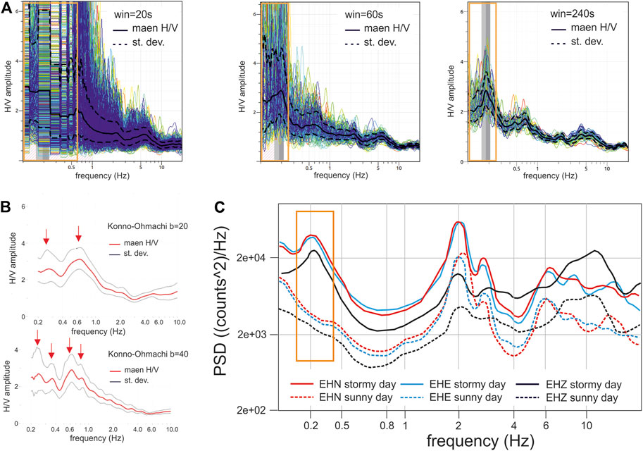
FIGURE 4. Panel (A) example of ambient noise HVSRs (Nakamura, 1989) calculated at IV. MILN station during a non-working day (i.e., 8th December 2021) using time sub-windows of increasing length of 20, 60 and 240 s, respectively; Panel (B) example of ambient noise HVSRs (Nakamura, 1989) calculated at IV. MILN station considering FFTs obtained by the Konno-Ohmachi smoothing windows, with b equal to 20 and 40; Panel (C) example of Power Spectral Density (PSD) calculated at IV. MILN station from ambient noise recorded at the end of October 2021 during a sunny and a stormy day, respectively.
To calculate the HVSRs, for each single sub-window the spectral ratio between the root-mean-square average spectra of the horizontal components over the vertical components is calculated (Nakamura, 1989). Finally, the mean and standard deviation are computed.
For completeness, the results obtained for the 33 ambient noise measurements are illustrated in the Supplementary Material, in figures from Supplementary Figure S1–S6, while Supplementary Table S1 indicates all frequency peaks (i.e., pk) and related uncertainties recognized at urban scale by multiple measurements.
Figure 5 (panel A) shows the results in terms of mean ± standard deviations (black solid and dotted lines, respectively) of the 33 ambient noise measurements, together with the mean HVSR curves obtained from independent sets of measurements performed in the northern (i.e., North of M002, Figure 2, panel A), central and southern (i.e., South of M026, Figure 2, panel A) parts of the urban area, respectively, and the mean HVSR curves representative of the seismic passive arrays performed at North Park, Giuriati sports center and Vettabbia park (Figure 2, panel A).
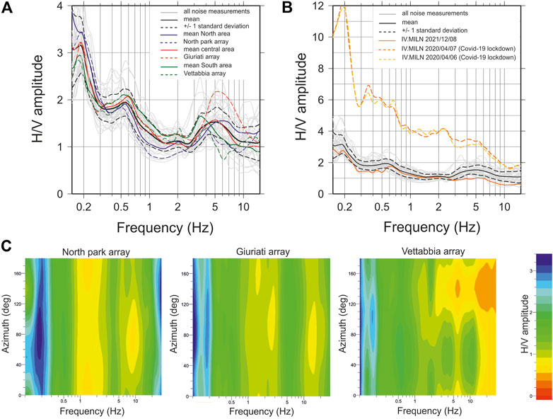
FIGURE 5. Panel (A) HVSRs relative to the 33 new ambient noise measurements (light grey) performed in the Milan urban area from March to June 2021 (in black mean amplification and ±1 standard deviation). Blue, red and green solid lines indicate the mean amplification functions for the north, central and south parts of the target area. Blue, red and green dotted lines indicate the amplification functions for the three target sites of North Park (north of the area), Giuriati (center part) and Vettabbia park (south of the area); Panel (B) comparison in terms of HVSRs between the new ambient noise measurements (light grey; in black mean amplification and ±1 standard deviation) and the results obtained at IV. MILN station using time windows selected both recently (i.e., December 2021) and during the Covid-19 lockdown (i.e., April 2020). Panel (C) directional ambient noise HVSRs obtained for North Park (left), Giuriati (center) and Vettabbia park (right).
In general, the HVSR curves (Figure 5, panel A) show a high degree of coherence, which showed 3 main amplified bands of frequency that are from 0.17 to 0.23 Hz (pk1, Supplementary Table S1), from 0.48 to 0.66 Hz (pk2, Supplementary Table S1) and from 3.2 to 7.6 Hz (pk3, Supplementary Table S1). In general, the HVSR curves show a slight decrease in frequency of the three main peaks moving from the Northern to the Southern part of the area.
Considering, the SESAME (2004) criteria for clear HVSR peaks, pk1 is the resonance frequency that shows a more reliable peak, with 2–4 satisfied criteria for about 70% of the measuring points (Supplementary Table S1). Pk3, instead, is the resonance peak that shows the highest number of satisfied criteria for a clear HVSR peak (5 satisfied criteria, Supplementary Table S1), even if for a lower percentage of measuring points (from 3 to 5 of satisfied criteria for about 40% of measuring points, Supplementary Table S1). Pk2 is the resonance frequency having more uncertainties concerning clear HVSR peaks. In particular, concerning the HVSR amplitude, except pk1, which shows values > 2 for the 80% of the measuring points (i.e., the lower bound for significant peaks), at higher frequency more variability is observable. All frequency peaks showing amplitude >2 are indicated in bold in Supplementary Table S1.
In general, the HVSRs variability in terms of both resonant peaks and amplitude at high frequency (>1 Hz) could be associated with very local factors (i.e., local soil conditions, anthropic ambient noise levels etc.). For example, Figure 5 (panel B) shows a comparison between the HVSR calculated for the new 33 ambient noise measurements and the HVSR calculated from ambient noise recorded by the Trillium 40s installed at IV. MILN station, both during a non-working day (i.e. 8th December 2021) and during the lockdown against the Covid-19 pandemic (i.e. April 2020, Sunday 6th and April 2020, Monday 7th). This example shows the strong influence in an urban area of the anthropic noise on the vertical component of motion and, consequently, on the final results in terms of HVSR. The relative Power Spectral Density (PSD) is shown in the Supplementary Material (Supplementary Figure S7).
At low frequency (<1 Hz), the noise level could be affected by variations due to differences in the environmental conditions during the period when the measurement is performed (e.g., Marzorati and Bindi, 2006).
Finally, to detect possible polarization effects of the horizontal components, Fourier spectra are computed by rotating the north–south (N-S) and east-west (E-W) noise components clockwise from the North, from 0° to 180° with step of 10°. For each direction, the HVSR is computed considering the ratio between the Fourier spectrum of each rotated horizontal component and the Fourier spectrum of the vertical component. Figure 5 (panel C) shows the rotated HVSR obtained at North park, Giuriati sports center and Vettabbia park, where in all cases just negligible polarization in directions ranging from 40°N to 120°N is detected around 0.2 Hz.
Figure 6 shows, in the map, the variability of the more relevant frequency peaks detected at high (pk3, panel A) and low (pk1, panel B) frequency, highlighting decreasing values moving from the northern to the southern part of the studied area.
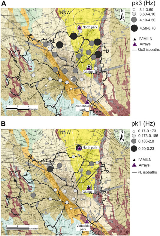
FIGURE 6. Resonance frequency intervals for pk3 (panel A) and pk1 (panel B) HVSR ambient noise peaks (see Supplementary Table S1) superimposed on the geological map of the area (Figure 2, panel A). Measuring points that not satisfied the SESAME (2004) criteria for clear HVSR peaks (see black and dark grey cells in Supplementary Table S1) are not considered. Top and bottom panels also indicate the isobaths of Qc3 (base of the upper Padano Supersynthem, see Figure 2B and Table 2) and PL (base of Pliocene, Figure 2C and Table 2) unconformities as recognized by the Geomol project (2015).
The results obtained from ambient noise HVSRs are compared with those from earthquake HVSRs (e.g., Lermo and Chavez-Garcìa, 1993), calculated considering the set of seismic events reported in Table 1. The selected earthquakes, with magnitude (Mw) ranging from 3.7 to 5.8, are recorded by the IV. MILN station and occurred in the Po Plain area and surroundings from the 1st January 2012 until today. The velocimetric data selected for the analyses are downloaded from the EIDA web site (http://www.orfeus-eu.org/data/eida/).
The simple data processing involved the application of a baseline operator to the entire record to obtain the zero-mean signal and subsequently to remove any linear trends, a tapering cosine function (0.05%) applied at the beginning and the end of each selected window and a 4th order Butterworth band-pass acausal (Boore and Akkar, 2003) filter to remove the high and low-frequency noises; for each analysed event the filter cut-off thresholds are selected by a visual inspection.
Given the long-period effects due to the low frequencies propagation in the Po plain basin during the 2012 Emilia seismic sequence (e.g., Luzi et al., 2013), the earthquakes HVSRs are computed on both the S-waves train and the coda. Time windows from 10 to 20 s are selected for the S-waves starting from their onset after a visual inspection. Time lengths for the surface train waves are determined through a time-frequency analysis on each single earthquake. Finally, coda windows ranging from 15 to 60 s are selected at the end of the S-phase depending on each earthquake’s magnitude, distance and ray-path.
An example of propagation effects on train waves crossing along the Po plain alluvial deposits is shown in Figure 7 (bottom panels), where the EW velocimetric waveforms recorded at IV. MILN station during the 20th May 2012, Mw 5.8, Emilia mainshock (Repi 169 km) and during the 18th December 2021, Dalmine, Mw 3.9, event (Repi 35 km, see Table 1) are shown; in the first case, the example shows the generation of surface waves with the consequence of long earthquake ground motion duration and PGV recorded on coda. In the second case, the hypocentre is located at a depth of 31 km and the source to site distance is 35 km, so no surface waves are generated and the PGV is found on the S-phase.
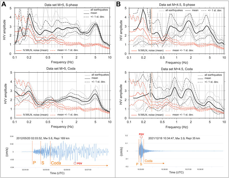
FIGURE 7. Earthquake HVSRs calculated on the events listed in Table 1. Panel (A) shows the results obtained on a sub set of events with magnitude >5 and epicentral distances from 127 to 191 km, while panel (B) indicates the results obtained considering events with magnitude <4.5 and epicentral distances from 8 to 143 km; the vertical orange dotted lines indicate the lower limit for stable HVSR curves obtained by using the available local earthquakes. The epicentres of the considered events are reported in the panel (B) of Figure 1. Bottom panels show two examples of near and far field waveforms recorded at IV. MILN station for the 2012/12/18 Dalmine Mw 3.9 event (right) and for the 2012/05/20 Emilia Mw 5.8 mainshock (left).
In detail, the HVSRs are calculated by splitting the earthquakes in two different sets of data, the first including the 2012 Emilia earthquakes with Mw > 5, epicentral distances ranging from 148 to 191 km (Table 1) and homogeneous azimuth of ∼290°N (Figure 1, panel B); the second including earthquakes occurring mainly at the edge of the basin, with Mw < 4.5, maximum epicentral distance of 142 km (Table 1) and sparse azimuths in the range 2°–352°N (Figure 1, panel B).
The earthquakes HVSRs are shown in Figure 7, where panels A, B show the curves for the higher and lower magnitude set of events, respectively. In particular, top and central panels show the results in terms of mean amplitude calculated from S-phase and coda, respectively. The results obtained considering the ambient noise and the set of earthquakes with magnitude >5 show that the two HVSR curves agree at frequencies <0.5 Hz, particularly considering the coda waves for the higher magnitude set of events.
In case of the available local earthquakes, characterized by short distances and low magnitude, the windows lengths do not always assure the calculation of stable HVSR curves for frequencies lower than ∼0.5 Hz (Figure 7, right panels). This issue is even more relevant in case of high levels of ambient noise, such as at the IV. MILN station during working days (i.e., −110 < dB < −90 in the range 1–20 Hz).
The most relevant result comparing of earthquake and ambient noise HVSRs is that, at frequencies between 1 and 2 Hz, the ambient noise HVSRs do not show any amplification peak. In contrast, S-phase and coda depict clear amplification peaks for both set of events. Concerning the amplitude values, earthquakes HVSRs calculated both from S-phase and coda show in general higher amplitudes with respect to ambient noise, in particular for frequencies >0.5 Hz.
Concerning the possible influence of the different azimuths of the local earthquakes reported in Table 1, just in case of the two events of Mw = 3.9, recorded at IV. MILN station on 2021/12/18 10:34:47 (epicentral distance 35 km, depth 26 km and azimuth 293°N) and on 2020/12/17 15:59:22 (epicentral distance 8 km, depth 56 km, azimuth 83°N) higher amplitudes along the related ray-paths are detected on S-phase in the frequency range 1–8 Hz.
As in the case of ambient noise HVSRs, no polarization phenomena due to the recording site are observable from earthquake signals.
To characterize the shear wave velocity with depth, active and passive geophysical tests are carried out.
Two Multichannel Analyses of Surface Waves (MASW, Park et al., 1999) are performed at North public park and at Vettabbia public park using in both cases 24 vertical geophones with eigen natural frequency of 4.5 Hz and a vertical impact source (6.8 kg hammer). In both sites, the geophones are set out in a linear array varying the inter geophonic distance from 2.5 to 5 m (total length of 60 and 120 m respectively) and using a minimum offset moving from 5 to 10 m. The linear arrays allow investigating depths ranging from 30 to 35 m. The Rayleigh wave dispersion of the acquired data set is obtained from the stacking of 7 shots. For each shot, a sampling frequency of 2000 Hz and a time of acquisition of 2 s are chosen. To generate the phase velocity spectrum of Rayleigh waves, the phase shift algorithm (Park et al., 1998) is used.
In general, as expected, in the configuration with the greater geophonic inter distance (5 m) an improvement in signal correlation is observed in the low frequency phase velocity spectrum. In particular, at Vettabbia Park, in the configuration with the smaller geophonic inter distance (2.5 m) an improvement in signal correlation is also observed in the high frequency phase velocity spectrum (20–30 Hz). The cause of this observation is probably due to the attenuation properties of the more superficial soil layers that resulted, from local geognostic investigations (https://www.geoportale.regione.lombardia.it/), to be mostly incoherent fine deposits. From the phase velocity spectra obtained with the two configurations (5–2.5 m), the fundamental mode picking covered the frequency range 6–30 Hz at Vettabbia park and the frequency range 5.5–30 Hz at North park (Supplementary Figures S8 and S9 respectively). The Vs.30 calculated from MASW at North and Vettabbia park results equal to 345 m/s and to 265 m/s respectively, allowing classifying the analysed sites in C class (i.e. Vs.30 < 360 m/s) of Italian (NTC, 2018) and European (CEN, 2004) seismic codes.
To define S-wave velocity profiles for larger depths, 4 different microtremor arrays, with increasing apertures and different layouts are installed at North public park (Figure 8, panel A), Giuriati sports center, very close to the IV. MILN station (Figure 8, panel B), and Vettabbia public park (Figure 8, panel C). At Giuriati sports center, two microtremor arrays are carried out using a circular geometry with radii of 12 and 50 m, respectively (Figure 8, panel B). The layout of the two arrays consisted of a central receiver surrounded by 8 stations deployed with an angular distance of 45°. The instrumentation comprised Lennartz-5s high-sensitivity (400 V/m/s) velocimeters coupled with a 24-bit Reftek 130 three-channel digitizer. The sampling frequency is set at 100 Hz, with the recording period for each array of 3 h.
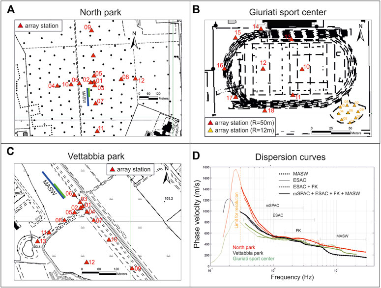
FIGURE 8. Panel (A) location of the MASW active surveys and of the 2D passive array performed at North Park; Panel (B) location of the two 2D passive microtremor arrays performed at Giuriati sports center; Panel (C) the same as in panel (A), but for Vettabbia public park; Panel (D) Rayleigh-wave dispersion curves from 2D passive microtremor array and MASW surveys.
For both North and Vettabbia public parks, one microtremor array is set up using the layouts reported in Figure 8 (panel A, C) and 14 Lennartz-5s high-sensitivity (400 V/m/s) velocimeters coupled with a 24-bit Reftek 130 three-channel digitizer. The sampling frequency and recording period are the same as that used at Giuriati. In this case, the two types of geometry enable work with inter distances among sensors in the range 5–600 m.
For each array, the first step of the analysis consists of a visual inspection of the recordings at each station. In particular, in order to identify malfunctioning and to select suitable signal windows for the surface wave analysis, the quality of the recording is evaluated by analysing the signal stationarity in the time domain, the relevant unfiltered Fourier spectra and the HVSR variation over time. During surface wave investigation, it is common practice to verify the reliability of the one-dimensional site structure assumption (Aki, 1957; Okada, 2003). For this reason, we estimated the HVSR at each station of the array and the stability of HVSR throughout the array stations is in the range of frequency (0.2–30 Hz). The analyses use synchronized signal windows, with lengths ranging from 60 to 120 s, extracted from the available recordings, avoiding time windows affected by local disturbances.
The Rayleigh wave dispersion curve relative to the fundamental mode is calculated for each seismic array, taking account of the vertical ground-motion components, using the modified spatial autocorrelation (mSPAC) method (Bettig et al., 2001), the f-k (frequency-wavenumber) beamforming method (Capon 1969; Lacoss et al., 1969) and the ESAC (Extended Spatial Auto Correlation) method (Ohori et al., 2002; Okada 2003). Although the f-k methods are considered stable and robust algorithms, the mSPAC and ESAC methods give reliable estimates of the dispersion characteristics within a larger frequency band. In any case, the use of various combinations is always advisable (Bard 2005; Parolai et al., 2006; Puglia et al., 2011; SESAME, 2004).
It is worth mentioning that in this case no higher modes of vibration are detected. It is well known that by recognizing just the fundamental mode of ellipticity, it is generally difficult to correct for the energy of SH and Love waves present in the horizontal components of the ambient vibration wavefield (e.g., Poggi and Fäh, 2010). In this way, the quality of results also depends on the number of the available receivers, on the quality of the sensors installation, on the selected array geometry and, in particular, from the available levels of background ambient noise (Supplementary Figure S7). Moreover, in our case, also the application of the high-resolution frequency-wavenumber analysis and the use of the three-component of motion (e.g., Lai et al., 2020) does not allow to improve the results obtained by using the vertical component.
At Giuriati sports center, the experimental dispersion curve is obtained by using the f-k and mSPAC methods; in particular, the microtremor arrays with radii equal to 12 and 50 m, allow the definition of the dispersion curve in the intervals ∼2.5–18 Hz and ∼0.4–3.5 Hz, respectively (Figure 8, panel D).
At North and Vettabbia public parks, the experimental dispersion curves are obtained by using the f-k, mSPAC and ESAC methods; in these cases, the analyses on microtremor arrays allow defining the dispersion curves in the intervals ∼0.3–3.0 Hz and ∼0.3–3.5 Hz, respectively; at higher frequencies, the dispersion curves are obtained by the interpretation of the MASW surveys in the intervals ∼5.5–30 Hz and ∼6.0–30 Hz, respectively (Figure 8, panel D).
The inversion procedure to obtain the 1D velocity profile is performed using the nearest neighborhood algorithm, as implemented in the Dinver software (Wathelet et al., 2008). To obtain the best results from the available data, at each target site a joint inversion of the experimental dispersion and the ellipticity curves is carried out, since the single station HVSR contains information on the mean S-wave velocity and the thickness of the sedimentary cover (Parolai et al., 2005). The ellipticity curves are evaluated by using the single station analysis (HVSR), selecting of the main peaks or the associated flanks, dividing the amplitude by √2 to reduce the Love-wave and body wave contributions (Fäh et al., 2001; Fäh et al., 2003). At Vettabbia park and Giuriati sports center, the inversion procedure to obtain the Vs. profiles is constrained by using the resonance peaks around 0.17 and 0.19 Hz respectively, while at North park a portion of HVSR curve in the range 0.2–0.8 Hz is used.
The Vs. profiles obtained for the three sites are shown in Figures 9, 10, 11 (panels A). Supplementary Figure S8 shows a detail of the Vs. profiles in the first 400 m of depth. The profiles are calculated using the dispersion curves obtained both from the passive arrays (Figures 9–11, panels B) and the active multichannel analysis of the surface waves, while the ellipticity contribution is estimated from a selected portion of the ambient noise HVSR curves (Figures 9–11, panels C).
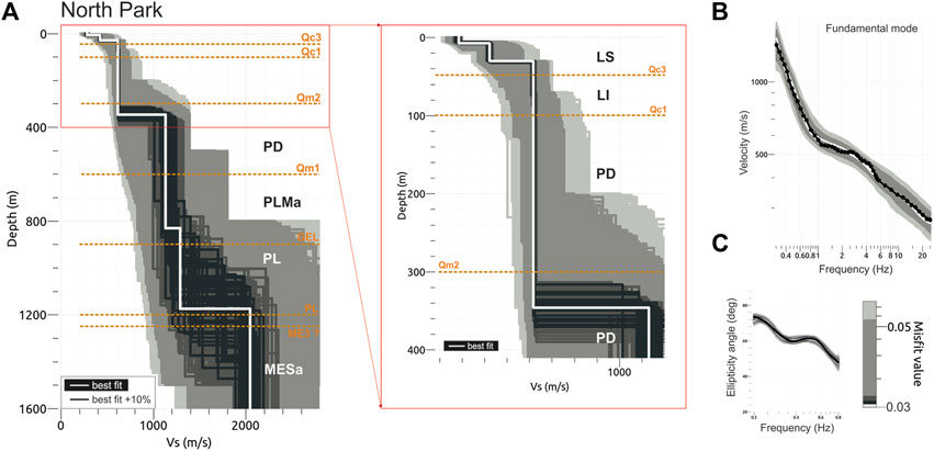
FIGURE 9. Panel (A) Vs. shear wave velocity profile obtained from the joint inversion (Rayleigh-wave dispersion curve and ellipticity curve) at North park. The main chrono stratigraphic units and the related unconformities (GeoMol Team, 2015), as reported in Figure 2 (Panels B, C) and Table 2, are also indicated. The central panel shows a detail of the Vs. shear wave velocity profile in the first 400 m of depth. Panel (B) experimental Rayleigh-wave dispersion (black dotted line) relative to the fundamental mode of vibration compared to the theoretical models (grey scale lines). The white line indicates the best-fit. Panel (C) experimental ellipticity curve (black line) obtained from a portion of ambient noise HVSR in the frequency range 0.2–0.8 Hz. Grey scale lines indicate the theoretical models. White line indicates the best fit.
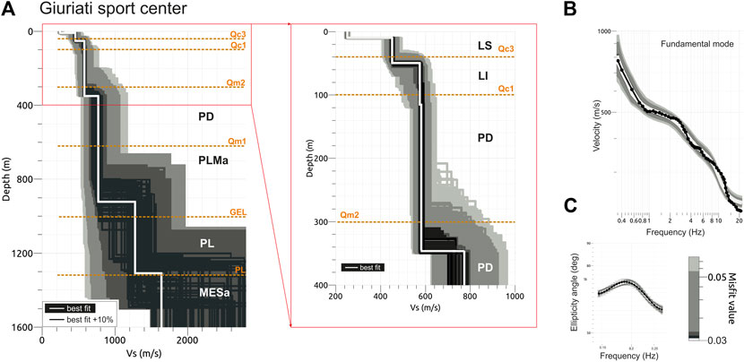
FIGURE 10. The same as for Figure 9, but considering the same analyses performed at Giuriati sports center.
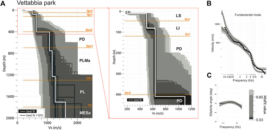
FIGURE 11. The same as for Figure 9, but considering the same analyses performed at Vettabbia public park.
The Vs. profile shows, in general, a similar trend of Vs. with depth and an increasing depth of the main contrasts of impedance towards South.
In particular, all Vs. profiles show a superficial layer with Vs. lower than 250 m/s and a first significant increase of Vs. to ∼420 m/s (Vettabbia park), ∼440 m/s (Giuriati sports center) and ∼500 m/s (North park) at depths ranging from ∼10 m (North park) to ∼20 m (Vettabbia park).
A second slight increase of Vs. is observable at depth of ∼35 m (North park), ∼45 m (Giuriati sports center) and ∼80 m (Vettabbia park), respectively, where the Vs. approaches the value of ∼600 m/s at all investigated sites.
The Vs. values keep constant before a third interface located at depths ranging from ∼300 m (North Park and Giuriati sports center) to ∼400 m (Vettabbia park); at all sites, the Vs. values reach or exceed 800 m/s, that correspond to the engineering bedrock (i.e., site class A, Vs.30 > 800 m/s) according to the European (CEN, 2004) and the Italian (NTC, 2018) seismic codes.
At larger depths, ranging from ∼850 m (North park) to ∼1250 m (Vettabbia park), the Vs. values reach ∼1150 m/s to ∼1250 m/s at all investigated sites. The deepest and observable Vs. interface is located at depths varying from ∼1200 m (North park) to ∼1700 m (Vettabbia park), although associated with large uncertainties. At these depths, the Vs. profile of the Giuriati sports center (Figure 10, panel A) follows an intermediate trend with respect to the results obtained at North (Figure 9, panel A) and Vettabbia (Figure 11, panel A) parks.
For all investigated sites, both the Vs. values and the depths of the main interfaces appear better constrained down to ∼400 m. In particular, in the uppermost 30 m the Vs. values are constrained by the dispersion curves obtained by both active and passive measurements, while the available stratigraphy from the shallow (https://www.geoportale.regione.lombardia.it/) and deep wells (Carg project, ISPRA et al., 2016; ViDEPI project, 2009), and the available literature (e.g., De Franco et al., 2009; Scardia et al., 2012) allow us to constrain the geological model. In general, the uncertainties of the Vs. models increase with increasing depths, in particular in the southern part of the city (i.e., Vettabbia park), where a limited amount of information is available. The Vs. values and the corresponding thickness of the model showing the best fit (white lines in Figures 9–11, panels A) are reported in Table 3.
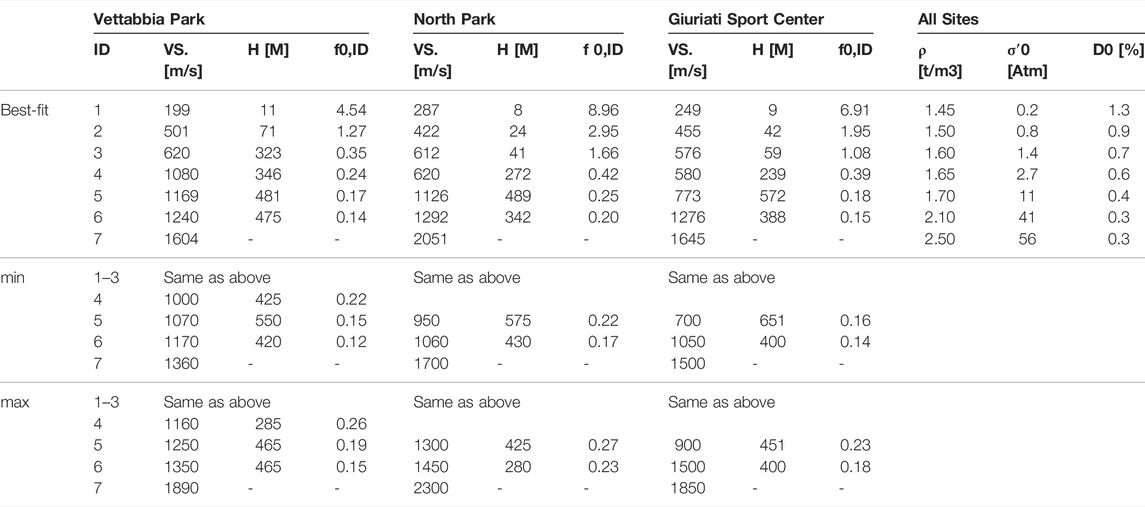
TABLE 3. Shear-wave velocities (VS) and layer thickness (H) used for 1D modelling at North Park, Giuriati sports center and Vettabbia park, together with the relative theoretical fundamental modes (f0(ID)). The f0(ID) values evidenced in bold indicate seismic impedance-contrasts between subsequent layers greater than 1.5. Values for unit weight (ρ), mean effective stress (σ′0) and damping at low-strains (D0), at each layer (ID) are also reported.
Given the available ground-motion recordings (i.e., maximum PGA = 36 gal), a linear site response model (i.e., within the low-strain field) is preferred to validate the proposed shear wave velocity models (Figures 9–11, panels A), by comparing the theoretical transfer functions (TFs) and the fundamental modes with the resonance peaks highlighted by ambient noise and earthquake HVSRs. The 1D linear site response is done by means of the software SHAKE91 (Schnabel, 1972; Idriss and Sun, 1993; Schnabel et al., 1993). In Table 3, for each layer (ID) and site, are also reported the values of the theoretical resonance frequencies associated to the fundamental-modes f0,ID, obtained by the equation:
where HT,ID is the sum of the layer thicknesses (HID), starting from the topmost layer and moving towards, and VST,ID is the weighted average of shear-wave velocities over HT,ID, obtained by the equation:
where HID and VS,ID are the thickness and the shear-wave velocity, respectively.
Table 3 also indicates the values for unit weight (ρ), useful for the impedance-contrast calculation, together with an estimation of the mean effective stress (σ′0) at each layer (ID), to be used in the equation by Darendeli (2001) for the low-strain damping (D0) calculation. In particular, the parameters of the Darendeli equations are fixed to: plasticity index: 0.0%; over-consolidation ratio: 1.0; cycles of loading: 10; characteristic frequency: 1 Hz. The mean effective stress (σ′0) is estimated from unit weight (ρ) considering a coefficient of lateral earth pressure equal to 0.50.
It is well known that the choice of the seismic input for a low-deformation field is theoretically not relevant. Then, as the seismic input for modeling, a generic strong-motion waveform is selected, just characterized by enough energy to overcome the numerical limits of the software in the frequency band of interest (i.e., 0.1–10 Hz). In fact, the fundamental modes estimated by eq. (1) are within the same frequency band of about 0.1–10 Hz, for the numerical models in question.
Finally, in order to also account for the variations of both VS and H in the modeling, Table 3 reports the two further VS models min and max. These models represent the minimum and maximum limit of the envelope that includes all VS profiles (i.e., black lines in panels a of Figures 9–11) obtained with uncertainties of 10% with respect to the best-fit model (i.e., white line in panels A of Figures 9–11).
The theoretical transfer functions are computed using the best model, together with the min and max models and are plotted in Figure 12, applying the Konno-Ohmachi smoothing (1998) operator with b = 40. The TFs are compared with the ambient noise HVSRs; except in the case of Giurati sports centre, which is sited very close to IV. MILN (∼300 m), where the HVSR from earthquakes is considered (Figure 12D).
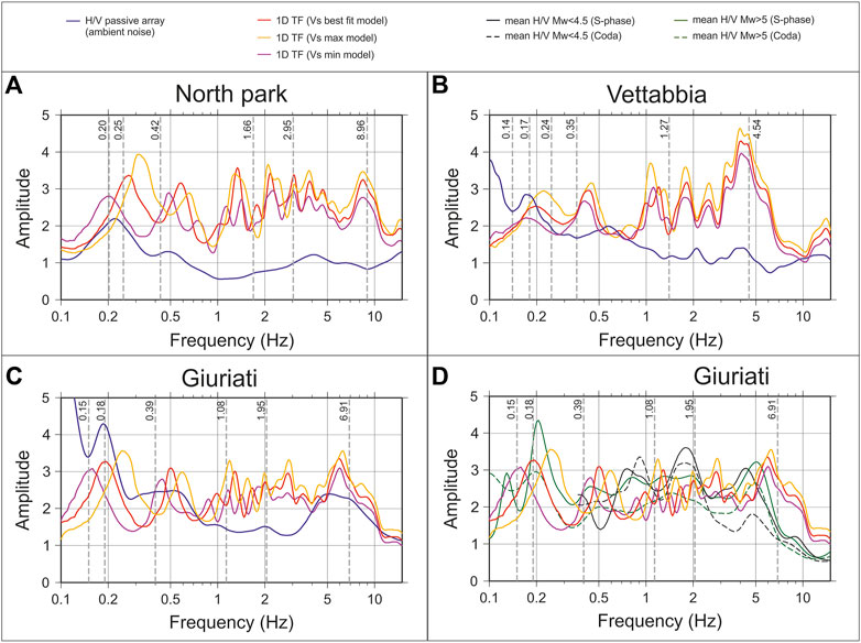
FIGURE 12. Theoretical transfer functions (TFs) obtained through 1D numerical modelling based on the linear field assumption at North Park (A), Vettabbia park (B) and Giuriati (C,D). Red, yellow and violet lines indicate the TFs obtained considering the best Vs-model and two Vs. profiles (i.e. min, max) that envelop the Vs. values with uncertainties of 10% with respect to the best fit. The vertical grey bars indicate for each site and layer (ID) the values of the theoretical resonance frequencies associated to the fundamental-modes f0,ID, obtained by eq. 1 (see also Table 3). All panels show the comparison with the amplitude functions obtained from ambient noise HVSR (blue lines). At Giuriati also earthquakes HVSRs are reported (D).
For all the analysed sites, the numerical model matches the resonance frequencies recognized by the experimental results, in particular for pk1 and pk3. On the contrary, more uncertainties are present in the range 0.5–3 Hz, where many peaks and valleys are present at different periods, as a consequence of the one-dimensional modeling adopted, which is composed by 7 homogeneous layers (Table 3). For all cases, a significant discrepancy in terms of peak amplitudes is evident by comparing the obtained TFs and the ambient noise HVSR curves.
In particular, both at North and Vettabbia parks the resonance frequencies obtained from the noise HVSRs at ∼ 0.2 Hz better match the resonant frequency of the TFs derived from the min model (Table 3). At Giuriati site, the mean earthquake HVSR agrees with TFs in terms of frequency and amplitudes, with except of the peak at ∼ 0.2 Hz, where the TFs slightly underestimate the experimental HVSRs obtained both from ambient noise and earthquakes.
In this paper, we present the work carried out to characterize the spatial variability of local soil conditions in the city of Milan and its surroundings and propose a seismo-stratigraphic model oriented to seismic site amplification. The model is derived from a combination of passive and active geophysical tests supported by a dense grid of geological and stratigraphic information from shallow and deep vertical wells and it is cross-checked with 1D numerical modeling.
The work consists of performing different geophysical tests; both active (i.e., MASW) and passive measurements are carried out to investigate both shallow and deep deposits. The passive analyses comprise 33 single-station ambient noise measurements and 4 microtremor arrays at 3 sites (i.e., North Park, Giuriati, Vettabbia) selected along a NNW-SSE alignment. The passive arrays are performed using different geometries and increasing aperture to explore the frequency range from 0.35 to 30 Hz. The geophysical analysis is supported by a subsoil model built along the NNW-SSE section after the collection and re-interpretation of all available geological and stratigraphic information and the documentation related to surficial and deep wells for exploration. Therefore, the resulting Vs. profiles, down to ∼1.8 km in depth, can be associated with the geophysical interfaces and stratigraphic discontinuities.
The transfer functions obtained from numerical models and cross-checked by experimental curves (HVSR from ambient noise and earthquakes) identify a first resonant frequency at about 0.2 Hz, namely the expression of a deep contrast of impedance, that we associate with the PL transition (Figures 10–12) between the Miocene sedimentary rocks (i.e., Gallare marls) and the overlying Pliocene deposits (i.e., Santerno clays).
The second contrast of impedance, relevant for site effects, is found at a depth between 300 and 400 m (Figures 10–12), at the transition between marine and continental sedimentation. In this case, a chronostratigraphic unconformity, Qm2 (Figures 10–12), is functional to geophysics, although the corresponding frequency is not evident from ambient noise HVSRs.
Shallower layers with low shear wave velocity (<250 m/s, Figures 10–12) result in high frequency peaks (between 3 and 8 Hz) that are evident in the ambient noise HVSRs.
A general trend, from all measurements, is the decrease in the frequency of the three main identified peaks, interpreted as the increase in depth of the deposits towards the centre of the Po plain, to the south.
Our hypotheses on the Vs. model should be verified due to the uncertainties and trade-off typical of the passive techniques (e.g., Lai et al., 2020). As an example, De Franco et al. (2009) interpret the subsoil of Milan by analysing a very deep active reflection profile, performed in the western part of the city and, in that case, except for superficial impedance contrast, the Vs. gradually increase down to ∼900 m without marked changes.
Another source of uncertainty can be the amplification peak around 0.2 Hz, which is interpreted as the coincidence with the microseismic long-period double-frequency peak by Marzorati and Bindi (2006) or Ferretti et al. (2013). Other authors, e.g., Paolucci et al. (2015), highlight a correlation between the amplitude values of the low-frequency peak and the sea-wave height, not observed for the high-frequency peaks. This issue could be resolved performing a generalised inversion of seismic data (e.g., Parolai et al., 2000; Ameri et al., 2011).
Moreover, the 1D approach which, in our opinion, is acceptable for the target area because surface stratigraphy is typically characterized by horizontal layers of alluvial deposits, does not account for the generation of surface waves, and the response of soil deposits is assumed to be predominantly related to SH waves propagating vertically from the underlying bedrock. Numerical modelling performed in the Po Plain highlighted that 2D and 3D effects can be significant because of the complex buried morphology of the basin (e.g., Vuan et al., 2011; Paolucci et al., 2015; Klin et al., 2019; Mascandola et al., 2021). In particular, due to the very large dimensions of the Po basin few attempts are available in the literature to objectively quantify 2D or 3D morphological effects on wave field propagation, in particular at low frequency, which makes this still an open issue.
This study will be useful for future site response assessments, numerical modelling of seismic-wave propagation, dynamic ground response analyses, and site-specific seismic hazard evaluation, contributing to future urban planning and risk mitigation (Eurocode 8, CEN, 2004; NTC, 2018).
The raw data supporting the conclusions of this article will be made available by the authors, without undue reservation.
This study started from an original idea of LL, MM and SL. MM, SL, GB, AL and CF contributed to the data acquisition of the passive seismic arrays and MAWS. All the Authors participated to the ambient noise single measurements performed in the urban area of Milan. MM analysed ambient noise and earthquakes data throught the HVSR method. MM, SL and RP worked on the ambient noise arrays to estimate the surface wave dispersion curves. MM and RP worked on the shear wave velocity profiles. RP performed the 1D numerical modeling. SL interpreted the geological and stratigraphic data and worked about the subsoil model.
National Institute of Geophysics and Volcanology (INGV).
The authors declare that the research was conducted in the absence of any commercial or financial relationships that could be construed as a potential conflict of interest.
All claims expressed in this article are solely those of the authors and do not necessarily represent those of their affiliated organizations, or those of the publisher, the editors and the reviewers. Any product that may be evaluated in this article, or claim that may be made by its manufacturer, is not guaranteed or endorsed by the publisher.
The authors thank the colleagues of INGV-Milano for the cooperation during the geophysical surveys, in particular Antonucci A., Manganello P., Mirenna S., Pessina V., Rizzo A. and Rovida A. Particular thanks to the Associate Editor, Roberto Paolucci, and to the reviewers who provided helpful reviews that improved this paper.
The Supplementary Material for this article can be found online at: https://www.frontiersin.org/articles/10.3389/feart.2022.915083/full#supplementary-material
Aki, K. (1957). Space and Time Spectra of Stationary Stochastic Waves, with Special Reference to Microtremors. Bull. Earthq. Res. Inst. 35, 415–457.
Ameri, G., Oth, A., Pilz, M., Bindi, D., Parolai, S., luzi, L., et al. (2011). Separation of Source and Site Effects by Generalized Inversion Technique Using the Aftershock Recordings of the 2009 L'Aquila Earthquake. Bull. Earthq. Eng. 9, 717–739. doi:10.1007/s10518-011-9248-4
Ansal, A., Tönük, G., and Kurtulucs, A. (2009). “Microzonation for Urban Planning,”. Earthquakes and Tsunamis, Geotechnical, Geological, and Earthquake Engineering. Editor A. T. Tankut (Dordrecht: Springer), Vol 11, 133–152. doi:10.1007/978-90-481-2399-5_9
Ansal, A., Kurtuluş, A., and Tönük, G. (2010). Seismic Microzonation and Earthquake Damage Scenarios for Urban Areas. Soil Dyn. Earthq. Eng. 30, 1319–1328. doi:10.1016/j.soildyn.2010.06.004
Aversa, S., and Crespellani, T. (2016). Seismic Microzonation: an Essential Tool for Urban Planning in Seismic Areas. Upl. J. Urban Plann Landsc. Environ. Des. 1 (1), 121–152. doi:10.6092/2531-9906/5035
Bard, P. Y. (2005). Site Effects Assessment Using Ambient Excitations (SESAME). WP 6: Derivation of Dispersion Curves. Grenoble: Technical report.
Beck, J. L., and Hall, J. F. (1986). Factors Contributing to the Catastrophe in Mexico City during the Earthquake of September 19, 1985. Geophys. Res. Lett. 13, 593–596. doi:10.1029/gl013i006p00593
Bettig, B., Bard, P. Y., Scherbaum, F., Riepl, J., Cotton, F., Cornou, C., et al. (2001). Analysis of Dense Array Measurements Using the Modified Spatial Auto-Correlation Method (SPAC). Application to Grenoble Area. Bol. Geofis. Teor. Appl. 42 (3-4), 281–304.
Bielak, J., Xu, J., and Ghattas, O. (1999). Earthquake Ground Motion and Structural Response in Alluvial Valleys. J. Geotechnical Geoenvironmental Eng. 125 (5), 413–423. doi:10.1061/(asce)1090-0241(1999)125:5(413)
Bigi, G., Costantino, D., Parotto, M., Sartori, R., and Scandone, P. (1990). – Structural Model of Italy. Firenze, Società Elaborazioni Cartografiche (S.EL.CA.), Consiglio Nazionale Delle Ricerche Progetto Finalizzato Geodinamica, Scala 1:500.000, 9 Fogli.
Bocherdt, R. D. (1970). Effects of Local Geology on Ground Motion Near San Francisco Bay. Bull. Seismol. Soc. Am. 60, 29–61. doi:10.1785/BSSA0600010029
Boore, D. M., and Akkar, S. (2003). Effect of Causal and Acausal Filters on Elastic and Inelastic Response Spectra. Earthq. Engng. Struct. Dyn. 32, 1729–1748. doi:10.1002/eqe.299
Capon, J. (1969). High-resolution Frequency-Wavenumber Spectrum Analysis. Proc. IEEE 57, 1408–1418. doi:10.1109/proc.1969.7278
Celikbilek, A., and Sapmaz, G. (2016). Risk Management and Microzonation in Urban Planning: an Analysis for Istanbul. Disaster Sci. Eng. 2 (2), 59–66.
Crespellani, T. (2014). Seismic Microzoning in Italy: a Brief History and Recent Experiences. Ing. Sism 31 (2), 3–31.
D’Amico, V., Picozzi, M., Baliva, F., Albarello, D., Menichetti, M., Bozzano, F., et al. (2006). “Test Sites in Europe for the Evaluation of Ground Motion Amplification: Site Response of the Gubbio Basin (Central Italy) Using Geological Data and Seismic Noise Measurements,” in Proceeding of the 1st European Conference on Earthquake Engineering and Seismology, Geneva, Switzerland (Geneva: Abstract Book), 301.
D’Amico, V., Picozzi, M., Baliva, F., and Albarello, D. (2008). Ambient Noise Measurements for Preliminary Site-Effects Characterization in the Urban Area of Florence, Italy. Bull. Seismol. Soc. Am. 98 (3), 1373–1388. doi:10.1785/0120070231
Darendeli, M. B. (2001). Development of a New Family of Normalized Modulus Reduction and Material Damping Curves. (PhD thesis). Austin, Texas: University of Texas. Available at: https://repositories.lib.utexas.edu/bitstream/handle/2152/10396/darendelimb016.pdf March, accessed 2022).
De Ferrari, R., Ferretti, G., Barani, S., and Spallarossa, D. (2010). Investigating on the 1920 Garfagnana Earthquake (Mw=6.5): Evidences of Site Effects in Villa Collemandina (Tuscany, Italy). Soil Dyn. Earthq. Eng. 30, 1417–1429. doi:10.1016/j.soildyn.2010.07.004
De Franco, R., Biella, G., Caielli, G., Berra, F., Guglielmin, M., Lozej, A., et al. (2009). Overview of High Resolution Seismic Prospecting in Pre-Alpine and Alpine Basins. Quat. Int. 204 (1-2), 65–75. doi:10.1016/j.quaint.2009.02.011
Dondi, L., Mostardini, F., and Rizzini, A. (1982). “Evoluzione sedimentaria e paleogeografia nella pianura padana,” in Guida alla geologia del margine appenninico-padano, Guida Geol. Reg. S.G.I. Editors G. Cremonini, and F. Ricci Lucchi (Bologna (Italy), 47–58.
Eurocode 8, CEN (2004). Eurocode 8: Design of Structures for Earthquake Resistance. P1: General Rules, Seismic Actions and Rules for Buildings. Draft 6, 522. Doc CEN/TC250/SC8/N335.
Fäh, D., Kind, F., and Giardini, D. (2001). A Theoretical Investigation of Average H/V Ratios. Geophys. J. Int. 145 (2), 535–549. doi:10.1046/j.0956-540x.2001.01406.x
Fäh, D., Kind, F., and Giardini, D. (2003). Inversion of Local S-Wave Velocity Structures from Average H/V Ratios, and Their Use for the Estimation of Site-Effects. J. Seismol. 7 (4), 449–467. doi:10.1023/b:jose.0000005712.86058.42
Ferretti, G., Zunino, A., Scafidi, D., Barani, S., and Spallarossa, D. (2013). On Microseisms Recorded Near the Ligurian Coast (Italy) and Their Relationship with Sea Wave Height. Geophys. J. Int. 194, 524–533. doi:10.1093/gji/ggt114
Furumura, T., and Kennett, B. L. N. (1998). On the Nature of Regional Seismic Phases-III. The Influence of Crustal Heterogeneity on the Wavefield for Subduction Earthquakes: the 1985 Michoacan and 1995 Copala, Guerrero, Mexico Earthquakes. Geophys. J. Int. 135 (3), 1060–1084. doi:10.1046/j.1365-246x.1998.00698.x
GeoMol Team(2015). in GeoMol – Assessing Subsurface Potentials of the Alpine Foreland Basins for Sustainable Planning and Use of Natural Resources – Project Report. Lf. U. Augsburg, 188.
Grazier, V., Shakal, A., Scrivner, C., Hauksson, E., Polet, J., and Jones, L. (2002). TriNet Strong-Motion Data from the M 7.1 Hector Mine, California, Earthquake of 16 October 1999. Bull. Seismol. Soc. Am. 92, 1525–1542. doi:10.1785/0120000925
Hailemikael, S., Amoroso, S., and Gaudiosi, I. (2020). Guest editorial: Seismic Microzonation of Central Italy Following the 2016-2017 Seismic Sequence. Bull. Earth. Eng. 18, 5415–5422. doi:10.1007/s10518-020-00929-6
Hanks, T. C. (1975). Strong Ground Motion of the San Fernando, California, Earthquake: Ground Displacements. Bull. Seismol. Soc. Am. 65 (1), 193–225. doi:10.1785/bssa0650010193
Hatayama, K. (2008). Lessons from the 2003 Tokachi-Oki, Japan, Earthquake for Prediction of Long-Period Strong Ground Motions and Sloshing Damage to Oil Storage Tanks. Journal.of Seismol 12, 255–263. doi:10.1007/s10950-007-9066-y
Hisada, Y., Aki, K., and Teng, T. L. (1993). 3-D Simulations of Surface Wave Propagation in the Kanto Sedimentary Basin, Japan Part 2: Application of the Surface Wave BEM. Bull. Seismol. Soc. Am. 83 (6), 1700–1720. doi:10.1785/BSSA0830061700
Idriss, I. M., and Sun, J. I. (1993). User’s Manual for SHAKE91: A Computer Program for Conducting Equivalent Linear Seismic Response Analyses of Horizontally Layered Soil Deposits. Davis, CA, USA: Center for Geotechnical Modeling, Department of Civil and Environmental Engineering, University of California.
ISPRA Geologico d’Italia, S., and Lombardia, R. (2016). in Carta Geologica d’italia alla scala 1:50.000, Foglio 118 Milano (con note illustrative). Editors V. A cura di Francani, A. Piccin, M. Credali, F. Berra, D. Battaglia, P. Gattinoniet al.
Joyner, W. B. (2000). Strong Motion from Surface Waves in Deep Sedimentary Basins. Bull. Seismol. Soc. Am. 90 (6B), S95–S112. doi:10.1785/0120000505
Kagawa, T., Zhao, B., Miyakoshi, K., and Irikura, K. (2004). Modeling of 3D Basin Structures for Seismic Wave Simulations Based on Available Information on the Target Area: Case Study of the Osaka Basin, Japan. Bull. Seismol. Soc. Am. 94 (4), 1353–1368. doi:10.1785/012003165
Kim, H.-S., Sun, C.-G., and Cho, H.-I. (2017). Geospatial Big Data-Based Geostatistical Zonation of Seismic Site Effects in Seoul Metropolitan Area. Int. J. Geo-Information 6 (6), 174. doi:10.3390/ijgi6060174
Klin, P., Laurenzano, G., Romano, M. A., Priolo, E., and Martelli, L. (2019). ER3D: a Structural and Geophysical 3-D Model of Central Emilia-Romagna (Northern Italy) for Numerical Simulation of Earthquake Ground Motion. Solid earth. 10 (3), 931–949. doi:10.5194/se-10-931-2019
Koketsu, K., Hatayama, K., Furumura, T., Ikegami, Y., and Akiyama, S. (2005). Damaging Long-Period Ground Motions from the 2003 Mw 8.3 Tokachi-Oki, Japan Earthquake. Seismol. Res. Lett. 76, 67–73. doi:10.1785/gssrl.76.1.67
Koketsu, K., and Miyake, H. (2008). A Seismological Overview of Long-Period Ground Motion. J. Seismol. 12 (2), 133–143. doi:10.1007/s10950-007-9080-0
Konno, K., and Ohmachi, T. (1998). Ground-motion Characteristics Estimated from Spectral Ratio between Horizontal and Vertical Components of Microtremor. Bull. Seismol. Soc. Am. 88, 228–241. doi:10.1785/bssa0880010228
Lacoss, R. T., Kelly, E. J., and Toksöz, M. N. (1969). Estimation of Seismic Noise Structure Using Arrays. Geophysics 34, 21–38. doi:10.1190/1.1439995
Lai, C. G., Poggi, V., Famà, A., Zuccolo, E., Bozzoni, F., Meisina, C., et al. (2020). An Inter-disciplinary and Multi-Scale Approach to Assess the Spatial Variability of Ground Motion for Seismic Microzonation: the Case Study of Cavezzo Municipality in Northern Italy. Eng. Geol. 274, 105722. doi:10.1016/j.enggeo.2020.105722
Laurenzano, G., Priolo, E., Mucciarelli, M., Martelli, L., and Romanelli, M. (2017). Site Response Estimation at Mirandola by Virtual Reference Station. Bull. Earthq. Eng. 15 (6), 2393–2409. doi:10.1007/s10518-016-0037-y
Lermo, J., and Chávez-García, F. J. (1993). Site Effect Evaluation Using Spectral Ratios with Only One Station. Bull. Seism. Soc. Am. 83 (5), 1574–1594. doi:10.1785/bssa0830051574
Liang, J. Z., Hao, H., Wang, Y., and Bi, K. M. (2009). Design Earthquake Ground Motion Prediction for Perth Metropolitan Area with Microtremor Measurements for Site Characterization. J. Earthq. Eng. 13 (7), 997–1028. doi:10.1080/13632460802687710
Liu, L., Chen, Q.-f., Wang, W., and Rohrbach, E. (2014). Ambient Noise as the New Source for Urban Engineering Seismology and Earthquake Engineering: a Case Study from Beijing Metropolitan Area. Earthq. Sci. 27 (1), 89–100. doi:10.1007/s11589-013-0052-x
Luzi, L., Pacor, F., Ameri, G., Puglia, R., Burrato, P., Massa, M., et al. (2013). Overview on the Strong-Motion Data Recorded during the May-June 2012 Emilia Seismic Sequence. Seismol. Res. Lett. 84 (4), 629–644. doi:10.1785/0220120154
Maddalena Michele, M., Raffaele Di Stefano, R., Lauro Chiaraluce, L., Marco Cattaneo, M., Pasquale De Gori, P., Giancarlo Monachesi, G., et al. (2016). The Amatrice 2016 Seismic Sequence: a Preliminary Look at the Mainshock and Aftershocks Distribution. Ann. Geophys. Fast track 59, 59. doi:10.4401/ag-7227
Marcucci, S., Milana, G., Hailemikael, S., Carlucci, G., Cara, F., Di Giulio, G., et al. (2019). The Deep Bedrock in Rome, Italy: a New Constraint Based on Passive Seismic Data Analysis. Pure Appl. Geophys. 176 (6), 2395–2410. doi:10.1007/s00024-019-02130-6
Martelli, L., and Romani, M. (2013). Microzonazione Sismica e analisi della condizione limite per l’emergenza delle aree epicentrali dei terremoti della pianura emiliana di maggio-giugno 2012, relazione illustrativa, Servizio geologico, sismico e dei suoli Regione Emilia Romagna (in Italian).
Marzorati, S., and Bindi, D. (2006). Ambient Noise Levels in North Central Italy. G-Cube 7 (9), 1–14. doi:10.1029/2006gc001256
Mascandola, C., Massa, M., Barani, S., Lovati, S., and Santulin, M. (2017). Long‐Period Amplification in Deep Alluvial Basins and Consequences for Site‐Specific Probabilistic Seismic‐Hazard Analysis: An Example from the Po Plain (Northern Italy). Bull. Seismol. Soc. Am. 107 (2), 770–786. doi:10.1785/0120160166
Mascandola, C., Massa, M., Barani, S., Albarello, D., Lovati, S., Martelli, L., et al. (2019). Mapping the Seismic Bedrock of the Po Plain (Italy) through Ambient‐Vibration Monitoring. Bull. Seismol. Soc. Am. 109 (1), 164–177. doi:10.1785/0120180193
Mascandola, C., Barani, S., Massa, M., and Albarello, D. (2021). New Insights on Long-Period (>1s) Seismic Amplification Effects in Deep Sedimentary Basins: the Case of the Po Plain (Northern Italy). Bull. Seism. Soc. Am. 111 (4), 2071–2086. doi:10.1785/0120200315
Massa, M., and Augliera, P. (2013). Teleseisms as Estimators of Experimental Long-Period Site Amplification: Application to the Po Plain (Italy) for the 2011 Mw 9.0 Tohoku-Oki (Japan) Earthquake. Bull. Seismol. Soc. Am. 103 (5), 2541–2556. doi:10.1785/0120120164
Milana, G., Bordoni, P., Cara, F., Di Giulio, G., Hailemikael, S., and Rovelli, A. (2013). 1D Velocity Structure of the Po River Plain (Northern Italy) Assessed by Combining Strong Motion and Ambient Noise Data. Bull. Earthq. Eng. 12 (5), 2195–2209. doi:10.1007/s10518-013-9483-y
NTC (2018). Aggiornamento delle Norme Tecniche per le Costruzioni. Part 3.2.2: Categorie di sottosuolo e condizioni topografiche, 42. Rome: Gazzetta Ufficiale n. del 20 febbraio 2018 (in Italian).
Miyazaki, S. I., Segall, P., Fukuda, J., and Kato, T. (2004). Space Time Distribution of Afterslip Following the 2003 Tokachi‐oki Earthquake: Implications for Variations in Fault Zone Frictional Properties. Geophys. Res. Lett. 31 (6), 410. doi:10.1029/2003gl019410
Molnar, S., Assaf, J., Sirohey, A., and Adhikari, S. R. (2020). Overview of Local Site Effects and Seismic Microzonation Mapping in Metropolitan Vancouver, British Columbia, Canada. Eng. Geol. 270, 105568. doi:10.1016/j.enggeo.2020.105568
Molnar, S., Sirohey, A., Assaf, J., Bard, P. Y., Castellaro, S., Cornou, C., et al. (2022). A Review of the Microtremor Horizontal-To-Vertical Spectral Ratio (MHVSR) Method. J. Seismol 16, 1–33. doi:10.1007/s10950-021-10062-9
Moya, A., Schmidt, V., Segura, C., Boschini, I., and Atakan, K. (2000). Empirical Evaluation of Site Effects in the Metropolitan Area of San José, Costa Rica. Soil Dyn. Earthq. Eng. 20 (1-4), 177–185. doi:10.1016/s0267-7261(00)00049-x
MPS Working Group (2004). Redazione della mappa di pericolosità sismica prevista dall’Ordinanza PCM del 20 marzo 2003Rapporto Conclusivo per il Dipartimento della Protezione Civile.
Mucciarelli, M., Gallipoli, M. R., Di Giacomo, D., Di Nota, F., and Nino, E. (2005). The Influence of Wind on Measurements of Seismic Noise. Geophys. J. Int. 161 (2), 303–308. doi:10.1111/j.1365-246x.2004.02561.x
Muttoni, G., Carcano, C., Garzanti, E., Ghielmi, M., Piccin, A., Pini, R., et al. (2003). Onset of Major Pleistocene Glaciations in the Alps. Geol 31 (11), 989–992. doi:10.1130/g19445.1
Nakamura, Y. (1989). A Method for Dynamic Characteristics Estimation of Subsurface Using Microtremor or the Ground Surface. QR Railw. Tech. Res. Inst. 30 (1), 25–33.
Ohori, M., Nobata, A., and Wakamatsu, K. (2002). A Comparison of ESAC and FK Methods of Estimating Phase Velocity Using Arbitrarily Shaped Microtremor Arrays. Bull. Seismol. Soc. Am. 92, 2323–2332. doi:10.1785/0119980109
Paolucci, E., Albarello, D., D’Amico, S., Lunedei, E., Martelli, L., Mucciarelli, M., et al. (2015). A Large Scale Ambient Vibration Survey in the Area Damaged by May-June 2012 Seismic Sequence in Emilia Romagna, Italy. Bull. Earthq. Eng. 13 (11), 3187–3206. doi:10.1007/s10518-015-9767-5
Park, C. B., Miller, R. D., and Xia, J. (1998). “Imaging Dispersion Curves of Surface Waves on Multi-Channel Record,” in SEG Technical Program Expanded Abstracts 1998 (Houston, TX, United States: Society of Exploration Geophysicists), 1377–1380.
Park, C. B., Miller, R. D., and Xia, J. (1999). Multichannel Analysis of Surface Waves. Geophysics 64, 800–808. doi:10.1190/1.1444590
Parolai, S., Bindi, D., and Augliera, P. (2000). Application of the Generalized Inversion Technique (GIT) to a Microzonation Study: Numerical Simulations and Comparison with Different Site-Estimation Techniques. Bull. Seismol. Soc. Am. 90 (2), 286–297. doi:10.1785/0119990041
Parolai, S., Picozzi, M., Richwalski, S. M., and Milkereit, C. (2005). Joint Inversion of Phase Velocity Dispersion and H/V Ratio Curves from Seismic Noise Recordings Using a Genetic Algorithm, Considering Higher Modes. Geophys. Res. Lett. 32, L01303. doi:10.1029/2004GL021115
Parolai, S., Richwalski, S. M., Milkereit, C., and Fäh, D. (2006). S-wave Velocity Profiles for Earthquake Engineering Purposes for the Cologne Area (Germany). Bull. Earthq. Eng. 4, 65–94. doi:10.1007/s10518-005-5758-2
Picozzi, M., Strollo, A., Parolai, S., Durukal, E., Özel, O., Karabulut, S., et al. (2009). Site Characterization by Seismic Noise in Istanbul, Turkey. Soil Dyn. Earthq. Eng. 29 (3), 469–482. doi:10.1016/j.soildyn.2008.05.007
Pieri, M., and Groppi, G. (1981). “Subsurface Geological Structure of the Po Plain, Italy,” in Progetto Finalizzato Geodinamica/Sottoprogetto “Modello Strutturale” (Rome: Consiglio Nazionale delle Ricerche Publ. N°), 414.
Poggi, V., and Fäh, D. (2010). Estimating Rayleigh Wave Particle Motion from Three-Component Array Analysis of Ambient Vibrations. Geophys. J. Int. 180 (Issue 1), 251–267. doi:10.1111/j.1365-246x.2009.04402.x
Puglia, R., Tokeshi, K., Picozzi, M., D’Alema, E., Parolai, S., and Foti, S. (2011). Interpretation of Microtremor 2D Array Data Using Rayleigh and Love Waves: the Case Study of Bevagna (Central Italy). Near Surf. Geophys. 9 (6), 529–540. doi:10.3997/1873-0604.2011031
Priolo, E., Romanelli, M., Barnaba, C., Mucciarelli, M., Laurenzano, G., Dall'Olio, L., et al. (2012). The Ferrara Thrust Earthquakes of May-June 2012: Preliminary Site Response Analysis at the Sites of the OGS Temporary Network. Ann. Geophy. 55 (4), 591–597. doi:10.4401/ag-6172
Ratchkovski, N. A., Hansen, R. A., Stachnik, J. C., Cox, T., Fox, O., Rao, L., et al. (2003). Aftershock Sequence of the Mw 7.9 Denali Fault, Alaska, Earthquake of 3 November 2002 from Regional Seismic Network Data. Seismol. Res. Lett. 74 (6), 743–752. doi:10.1785/gssrl.74.6.743
Regione Lombardia, Eni Divisione Agip (2002). Geologia degli acquiferi Padani della Regione Lombardia, a cura di Cipriano Carcano e Andrea Piccin. Firenze: S.EL.CA. (in Italian).
Ritter, J. R. R., Balan, S. F., Bonjer, K.-P., Diehl, T., Forbriger, T., Marmureanu, G., et al. (2005). Broadband Urban Seismology in the Bucharest Metropolitan Area. Seismol. Res. Lett. 76 (5), 574–580. doi:10.1785/gssrl.76.5.574
Rizzini, A., and Dondi, L. (1978). Erosional Surface of Messinian Age in the Subsurface of the Lombardian Plain (Italy). Mar. Geol. 27, 303–325. doi:10.1016/0025-3227(78)90037-3
Ronald Abraham, J., Lai, C. G., and Papageorgiou, A. (2015). Basin-effects Observed during the 2012 Emilia Earthquake Sequence in Northern Italy. Soil Dyn. Earthq. Eng. 78, 230–242. doi:10.1016/j.soildyn.2015.08.007
Rovida, A., Locati, M., Camassi, R., Lolli, B., and Gasperini, P. (2020). The Italian Earthquake Catalogue CPTI15. Bull. Earthq. Eng. 18 (7), 2953–2984. doi:10.1007/s10518-020-00818-y
Sambridge, M. (1999). Geophysical Inversion with a Neighbourhood Algorithm-I. Searching a Parameter Space. Geophys. J. Int. 138, 479–494. doi:10.1046/j.1365-246x.1999.00876.x
Sato, T., Graves, R. W., and Somerville, P. G. (1999). Three-dimensional Finite-Difference Simulations of Long-Period Strong Motions in the Tokyo Metropolitan Area during the 1990 Odawara Earthquake (MJ 5.1) and the Great 1923 Kanto Earthquake (MS 8.2) in Japan. Bull. Seismol. Soc. Am. 89 (3), 579–607. doi:10.1785/bssa0890030579
Scardia, G., De Franco, R., Muttoni, G., Rogledi, S., Caielli, G., Carcano, C., et al. (2012). Stratigraphic Evidence of a Middle Pleistocene Climate‐driven Flexural Uplift in the Alps. Tectonics 31 (6), 3108. doi:10.1029/2012tc003108
Schnabel, P. B., Lysmer, J., and Seed, H. B. (1993). SHAKE-91: Equivalent Linear Seismic Response Analysis of Horizontally Layered Soil Deposits. Berkeley, CA, USA: The Earthquake Engineering Online Archive NISEE E-Library.
Schnabel, P. B. (1972). SHAKE a Computer Program for Earthquake Response Analysis of Horizontally Layered Sites. Berkeley, CA, USA: EERC Report; University of California.
Schneider, J. A., Mayne, P. W., and Rix, G. J. (2001). Geotechnical Site Characterization in the Greater Memphis Area Using Cone Penetration Tests. Eng. Geol. 62 (1-3), 169–184. doi:10.1016/s0013-7952(01)00060-6
SESAME (2004). Guidelines for the Implementation of H/V Spectral Ratio Technique on Ambient Vibration Measurements, Processing and Interpretation. Available at: http://sesame-fp5.obs.ujf-grenoble.fr/Delivrables/Del-D23-HV_User_Guidelines.pdf Last accessed March, 2022).
Somerville, P. G., Collins, N. F., Graves, R. W., and Pitarka, A. (2004). “An Engineering Ground Motion Model for Basin Generated Surface Waves,” in Proc. 13th World Conference on Earthquake Engineering, Vancouver, B.C., Canada, August 2004.
Stephenson, W. J., Hartzell, S., Frankel, A. D., Asten, M., Carver, D. L., and Kim, W. Y. (2009). Site Characterization for Urban Seismic Hazards in Lower Manhattan, New York City, from Microtremor Array Analysis. Geophys. Res. Lett. 36 (3), 444. doi:10.1029/2008gl036444
Stucchi, M., Meletti, C., Montaldo, V., Crowley, H., Calvi, G. M., and Boschi, E. (2011). Seismic Hazard Assessment (2003-2009) for the Italian Building Code. Bull. Seismol. Soc. Am. 101, 1885–1911. doi:10.1785/0120100130
Sun, C.-G., Kim, H.-S., Chung, C.-K., and Chi, H.-C. (2014). Spatial Zonations for Regional Assessment of Seismic Site Effects in the Seoul Metropolitan Area. Soil Dyn. Earthq. Eng. 56, 44–56. doi:10.1016/j.soildyn.2013.10.003
Tarabusi, G., and Caputo, R. (2017). The Use of HVSR Measurements for Investigating Buried Tectonic Structures: the Mirandola Anticline, Northern Italy, as a Case Study. Int. J. Earth Sci. Geol. Rundsch) 106 (1), 341–353. doi:10.1007/s00531-016-1322-3
Tragni, N., Calamita, G., Lastilla, L., Belloni, V., Ravanelli, R., Lupo, M., Salvia, V., and Gallipoli, M. R. (2021). Sharing Soil and Building Geophysical Data for Seismic Characterization of Cities Using CLARA WebGIS: A Case Study of Matera (Southern Italy). Appl. Sci. 11 (9), 4254. doi:10.3390/app11094254
ViDEPI project (2009). Visibilità dei dati afferenti all'attività di esplorazione petrolifera in Italia Ministero dello sviluppo economico DGRME - Società Geologica Italiana, Assomineraria. Available at: https://www.videpi.com.
Vuan, A., Klin, P., Laurenzano, G., and Priolo, E. (2011). Far-Source Long-Period Displacement Response Spectra in the Po and Venetian Plains (Italy) from 3D Wavefield Simulations. Bull. Seismol. Soc. Am. 101 (3), 1055–1072. doi:10.1785/0120090371
Wang, J. H. (2008). Urban Seismology in the Taipei Metropolitan Area: Review and Prospective. TAO Terr. Atmos. Ocean. Sci. 19 (3), 2. doi:10.3319/tao.2008.19.3.213(t)
Wathelet, M., Chatelain, J.-L., Cornou, C., Giulio, G. D., Guillier, B., Ohrnberger, M., et al. (2020). Geopsy: A User-Friendly Open-Source Tool Set for Ambient Vibration Processing. Seism. Soc. Lett. 91 (3), 1878–1889. doi:10.1785/0220190360
Wathelet, M., Jongmans, D., Ohrnberger, M., and Bonnefoy-Claudet, S. (2008). Array Performances for Ambient Vibrations on a Shallow Structure and Consequences over V S Inversion. J. Seismol. 12, 1–19. doi:10.1007/s10950-007-9067-x
Keywords: milan (Italy), seismic site characterisation, seismostratigrahic model, vs. velocity profile, seismic array, MASW, HVSR (horizontal to vertical spectral ratio), 1D numerical modeling
Citation: Massa M, Lovati S, Puglia R, Brunelli G, Lorenzetti A, Mascandola C, Felicetta C, Pacor F and Luzi L (2022) Seismo-Stratigraphic Model for the Urban Area of Milan (Italy) by Ambient-Vibration Monitoring and Implications for Seismic Site Effects Assessment. Front. Earth Sci. 10:915083. doi: 10.3389/feart.2022.915083
Received: 07 April 2022; Accepted: 19 19 May 20222022;
Published: 14 June 2022.
Edited by:
Roberto Paolucci, Politecnico di Milano, ItalyReviewed by:
Alessandro Vuan, Istituto Nazionale di Oceanografia e di Geofisica Sperimentale, ItalyCopyright © 2022 Massa, Lovati, Puglia, Brunelli, Lorenzetti, Mascandola, Felicetta, Pacor and Luzi. This is an open-access article distributed under the terms of the Creative Commons Attribution License (CC BY). The use, distribution or reproduction in other forums is permitted, provided the original author(s) and the copyright owner(s) are credited and that the original publication in this journal is cited, in accordance with accepted academic practice. No use, distribution or reproduction is permitted which does not comply with these terms.
*Correspondence: M. Massa, bWFyY28ubWFzc2FAaW5ndi5pdA==
Disclaimer: All claims expressed in this article are solely those of the authors and do not necessarily represent those of their affiliated organizations, or those of the publisher, the editors and the reviewers. Any product that may be evaluated in this article or claim that may be made by its manufacturer is not guaranteed or endorsed by the publisher.
Research integrity at Frontiers
Learn more about the work of our research integrity team to safeguard the quality of each article we publish.